Superpixel Segmentation of Hyperspectral Images Based on Entropy and Mutual Information

Abstract

Superpixel segmentation (SS) methods have been proven to be feasible in improving the performance of hybrid algorithms on hyperspectral images (HSIs). In this paper, a superpixel segmentation algorithm based on the information measures with color histogram driving (IM-CHD) was proposed. First, Shannon entropy was applied to measure the image information and preliminarily select spectral bands. Mutual information (MI) is derived from the concept of entropy and measures the statistical dependence between two random variables. Also, MI can effectively identify the redundant spectral bands. Therefore, in this paper, both MI and color matching functions (CMF) were used to select the most useful spectral bands. Second, the selected spectral bands were combined into a false color image containing the main spectral information. A local optimization algorithm named “hill climbing” was used to achieve the superpixel segmentation. Finally, parameter selection experiments and comparative experiments were performed on two hyperspectral data sets. The experimental results showed that the IM-CHD method was more efficient and accurate than other state-of-the-art methods.

1. Introduction

Hyperspectral images (HSIs) contain full spectral and spatial information, and the formed three-dimensional data block can effectively reflect much ground object information that cannot be detected in wide-band multi-spectral images [1]. In recent years, the classification of hyperspectral images has received extensive attention in the field of remote sensing image processing. In addition, hyperspectral images have the characteristics of high dimension and high information redundancy. Therefore, dimensionality reduction and image preprocessing (such as image segmentation) are important.

At present, there are mainly two types of dimension reduction methods for hyperspectral images, i.e., feature extraction and band selection. Band selection is based on information measures and has been intensively studied. In the band selection method, Shannon entropy or its variations are typically used to evaluate image information. Shannon proposed a supervised band-selection algorithm, in which only the known class signatures were used while neither the original band nor a training sample was required [2]. Based on mutual information, Martínez-Usó et al. used a clustering method to select band and achieve dimensionality reduction [3]. Based on spatial entropy, Wang et al. proposed a hyperspectral band selection algorithm for supervised classification [4]. On the other hand, many methods perform feature extraction on hyperspectral images to achieve dimensionality reduction. For example, Chavez and Kwarteng proposed a selection method using principal component analysis (PCA) [5]. Wang et al. proposed a non-linear extraction method based on manifold learning [6]. The dimensionality of data can be reduced by finding the corresponding coordinates on low-dimensional manifold for the points in high-dimensional space. Chen et al. proposed a dimensionality reduction method for hyperspectral images based on sparse representation [7]. Jacobson et al. proposed a band transformation method that extends the color matching functions (CMF) to the entire image spectra, which provided a foundation for subsequent band selection [8].

In addition to the dimensionality reduction, hyperspectral image segmentation can also reduce the processing complexity of subsequent images. Acito et al. proposed an HSIs segmentation algorithm based on statistical approach [9]. The proposed algorithm was completely unsupervised and only relied on the spectral information. Veganzones et al. proposed a hyperspectral image segmentation method using a new spectral unmixing-based binary partition tree representation [10]. Rundo et al. proposed an intelligent image analysis framework for image enhancement, automatic global thresholding and segmentation [11]. However, the above traditional object-level segmentation algorithms have the common problem of under-segmentation, which has a significant impact on post-processing. In recent years, some researchers have proposed an over-segmentation scale called superpixel, which has adaptive sizes and shapes for different spatial structures. In the hyperspectral image classification process, segmentation using the superpixel method can effectively reduce the impact of the segmentation scale on the classification results [12]. Therefore, superpixel segmentation (SS) has become an important preprocessing method for HSIs. The concept of superpixel was firstly proposed by Ren et al. [13]. In recent years, new superpixel segmentation algorithms have been continuously proposed. Liu proposed an entropy rate-based objective function for superpixel segmentation. However, the proposed method was very computationally intensive and time consuming [14]. Bergh et al. proposed a superpixel segmentation algorithm via energy-driven sampling. However, the disadvantage of this method was that it cannot solve the problem of sudden colohr changes [15]. Zhang et al. proposed to pre-cluster the hyperspectral image for the non-linear graphs into Simple Linear Iterative Clustering (SLIC) superpixels, and then use the superpixels as the input of the dimensionality reduction algorithm [16]. In this method, only the first principal component map was used for segmentation, which may cause the loss of important information. Based on the region growth method in [17], Xu et al. proposed a super-pixel segmentation method [18]. In this method, on the basis of fast region growth, the low-dimensional representations of hyperspectral images were achieved without sacrificing subsequent classification performance. Rodarmel and Shan used principal component analysis as a preprocessing technique to classify hyperspectral images [19]. Based on super pixels, Zhang et al. proposed a hyperspectral image classification method to effectively identify the type of land cover [20]. Steven et al. proposed a band selection method to effectively visualize the spectral images [21]. The results showed that the superpixel segmentation scale had sufficient potential in hyperspectral image segmentation. Therefore, although superpixel segmentation is still under study, it has been proved to have promising prospects in HSIs segmentation.

In this paper, a new hyperspectral image superpixel segmentation algorithm (IM-CHD) was proposed, in which the new techniques and methods, such as band selection method based on information measures, CMF, and color histogram driving function, were used to achieve more accurate and effective HSIs segmentation. In our previous work [22], we have proposed an HSIs classification method based on information measure, and proved the effectiveness of obtaining the main spectra of HSIs through information measure. In this paper, we synthesize the false color image based on the spectral components selected by information measure, and realize the segmentation of hyperspectral image based on this. The results of this study have significant reference value in two major aspects.

(1)

The information measures theory, including entropy, mutual information, and normalized mutual information, was applied to superpixel segmentation for HSIs. When information measures were used in the superpixel segmentation, CMF was applied to HSIs at the same time. The combination of both information measures and CMF achieved dimensionality reduction of hyperspectral images. Thus, the superpixel segmentation based on information measures is different from the existing spectral band selection methods based on information measures.

(2)

As one of the most innovative and effective methods, superpixel segmentation based on color histogram driving and hill climbing optimization was used to segment the false color image obtained in previous steps.

2. Dimensionality Reduction of HSIs Based on Information Measures

Band selection refers to the selection of band images which have relevant or irrelevant information [23]. The entropy and mutual information were generally used as the criterion for the band selection [21]. The entropy of each spectral band was calculated to evaluate the amount of contained information in this band. A threshold was set to exclude the irrelevant spectral bands. Then CMF was used for spectrum segmentation and the mutual information was used for the final band selection. The process can be mainly divided into the following two steps.

2.1. Preliminary Selection of Spectral Bands Based on Entropy and Color Matching Function

Shannon first introduced the concept of entropy and mutual information [24]. It has been proven that Shannon’s information measures theory is very effective in reducing the dimensionality of high-dimensional data. In hyperspectral images, each channel is considered to be equivalent to a random variable $X$, and all the pixels of the channel are considered to be the events of $X$.

The entropy of a channel can be expressed as:

$$H\left(X\right)={\displaystyle \sum _{i=1}^{n}P\left(X_i\right)}{\log }_b\left[P\left(X_i\right)\right]$$

(1)

where $X_i$ is an event of $X$, $P\left(X_i\right)$ is the probability density of $X$, and $b$ is the order of the algorithm.

$X$ and $Y$ are two random variables with $n$ and $m$ values, respectively. The entropy of the joint event is:

$$H\left(X,Y\right)=-{\displaystyle \sum _{i=1}^n{\displaystyle \sum _{j=1}^{m}P\left(X_i,Y_j\right)}}\log P\left(X_i,Y_j\right)$$

(2)

where $P\left(X_i,Y_j\right)$ is the probability of the joint occurrence of first $X_i$ and then $Y_j$.

The mutual information between the two random variables $X$ and $Y$ is:

$$\begin{array}{c}I\left(X,Y\right)={\displaystyle \sum _{i=1\dots n,j=1\dots m}P\left(X_i,Y_j\right)\log \frac{P\left(X_i,Y_j\right)}{P\left(X_i\right)\cdot P\left(Y_j\right)}}\\ =H\left(X\right)+H\left(Y\right)-H\left(X,Y\right)\end{array}$$

(3)

where $H\left(X\right)$ and $H\left(Y\right)$ are the entropy of a random variable $X$ and $Y$, respectively, $H\left(X,Y\right)$ is the joint entropy of the two random variables, $X$ and $Y$.

Bell proposed the concept of the co-information [25] of three random variables, $X$, $Y$ and $Z$, which can be expressed as follows:

$$\begin{array}{c}I\left(X;Y;Z\right)=H\left(X,Z\right)+H\left(Y,Z\right)-H\left(X,Y,Z\right)\\ =-H\left(Z\right)-I\left(X,Y\right)\end{array}$$

(4)

where $H\left(X,Y,Z\right)$ stands for the joint entropy of three random variables $X$, $Y$ and $Z$.

This principle remains feasible for HSIs. The information of one channel can increase the mutual information between the other two channels. Thus, when the co-information is smaller, the amount of the shared information is larger. In the preliminary selection, the low-informative channels are removed. First, the entropy of each spectral band of the HSIs is calculated. Second, the local average value is defined by Equation (5).

$$\overline{H_m\left(B_i\right)}=\frac{1}{m}{\displaystyle \sum _{p=-m/2}^{m/2}H\left(B_{i+p}\right)}$$

(5)

In Equation (5), $m$ stands for window size which represents the size of the neighborhood. All the bands

ThetAll the meeting the condition in Equation 6 can be retained.

$$H\left(B_i\right)\in \left[\overline{H_m\left(B_i\right)}\times \left(1-\sigma \right);\overline{H_m\left(B_i\right)}\times \left(1+\sigma \right)\right]$$

(6)

In Equation (6), $\sigma$ is the threshold factor. The bands with higher entropy than their local average values are distinguished by the threshold factor, and these bands are considered to be irrelevant, as shown in Figure 1.

The window size $m$ and threshold factor $\sigma$ were appropriately selected based on the smoothness of the curve. When the entropy curve was smoother, the probability of an uncorrelated band was lower and there was a smaller number of bands outside the correlation range. In this case, both $\sigma$ and $m$ were set to small value in order to improve the precision. On the contrary, a sharper curve indicated that the neighboring channels were more different. In this case, a larger window size should be used.

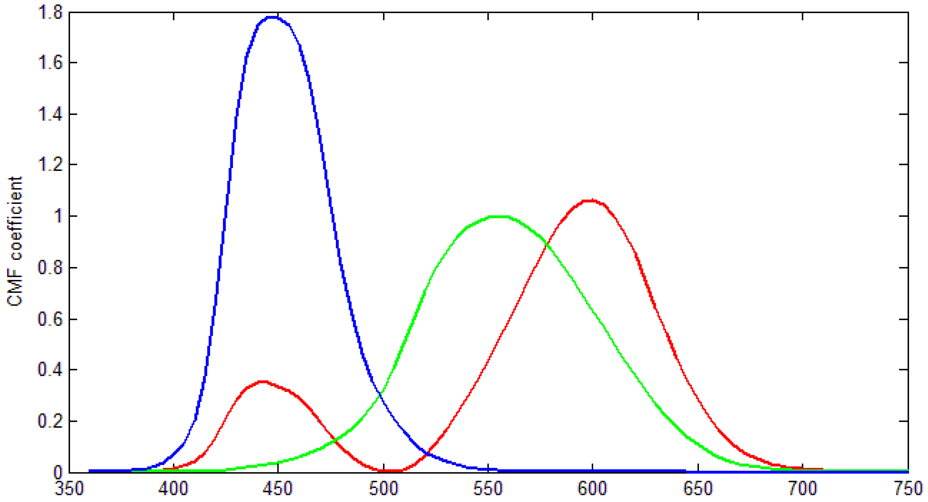
Then, the CIE 1931 supplementary standard colorimetric observer, i.e., CMF [26], was used to make a second selection of the spectral bands. Based on the experiments, the CMF for a particular wavelength was derived by determining the mixing ratio of the three primary colors of light (red, green, and blue) to generate the same impression as a monochromatic light at that wavelength. By applying the CIE color matching envelopes to the HSIs in the visible range, the HSIs can be visualized as a colorimetric ally correct image [8].

The wavelength was set to $\lambda =360$ nm in the first valid AVIRIS band and $\lambda =830$ in the last valid AVIRIS band. Then, linear interpolation was performed between the two bands to achieve HSIs stretch, as shown in Figure 2.

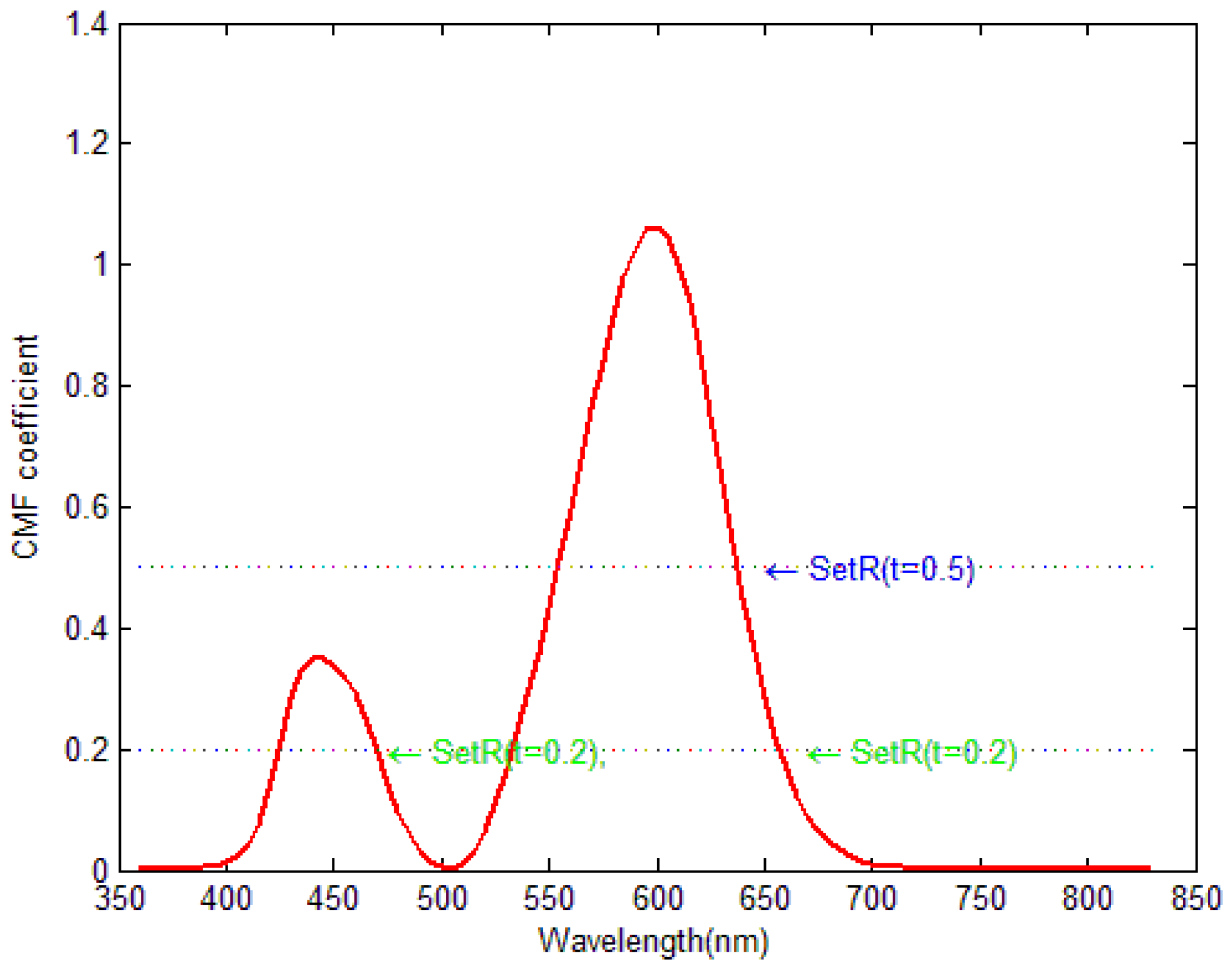
Finally, depending on the binarization threshold, i.e., $Se{t}_R^t$, $Se{t}_B^t$, and $Se{t}_G^t$, three segments were obtained, which were corresponding to the red, blue, and green primitive channels, respectively. The impact of $t$ is illustrated in Figure 3. In the figure, the horizontal lines represent the spectrum thresholds in two different cases ($t=0.1$ and $t=0.5$). The spectral bands with above-threshold CMF coefficients are retained.

In this paper, an automatic threshold method was adopted to determine $t$. The optimal threshold was defined as the value at which the amount of discarded information was maximized. $S_{discard}^t$ is defined as the set of channels removed by thresholding the CMF with $t$, and $S_{selected}^t$ is defined as the complementary set of $S_{discard}^t$. Then, the optimal value of $t$ can be obtained from Equation (7).

$$t_{opt}=\max \left(t\right)\mathrm{subject}\mathrm{to}H\left(S_{discard}^t\right)<H\left(S_{selected}^t\right)$$

(7)

2.2. Band Selection Algorithm Based on Mutual Information

The dimensionality reduction of the HSIs was achieved by optimizing two criteria, i.e., maximizing the amount of information and minimizing the redundancy. These two criteria need to be considered simultaneously.

Pla et al. used the normalized mutual information for band selection [27]. In this paper, the $kth$ order normalized information (NI) of the bandset $S=\left\{B_1,\cdots ,B_k\right\}$ was calculated as follows:

$$N{I}_k\left(S\right)=\frac{K\times I\left(S\right)}{{\displaystyle \sum _{i=1}^{k}H\left(B_i\right)}}$$

(8)

where $I\left(S\right)$ is the mutual information from $B_1$ to $B_k$, and $H\left(B_i\right)$ is the entropy of $B_i$.

From the above step, three segments can be obtained, i.e., ${\mathrm{Set}}_R^t$, ${\mathrm{Set}}_{\mathrm{B}}^{\mathrm{t}}$, and ${\mathrm{Set}}_{\mathrm{G}}^{\mathrm{t}}$. When the value of the mutual information between three bands $N{I}_3\left(\mathrm{S}\right)$ is smaller, the amount of useful information contained in the selected spectral bands is larger, and the dimensionality reduction effect is better. Thus, the minimum, second minimum, and up to $nth$ minimum values of $N{I}_3\left(\mathrm{S}\right)$ can be calculated based on the values of $x_{Rn},y_{Bn},z_{Gn}\left(x_{Rn}\in Se{t}_R^t,y_{Bn}\in Se{t}_B^t,z_{Gn}\in Se{t}_G^t,n=1,2,\dots 10\right)$. Finally, the $3n$ spectral bands are selected to composite the false color images. This method is not only convenient to configure, but also produce the images containing the main spectral information. The optimal value of $n$ was determined by experiments.

3. Superpixel Segmentation Based on Color Histogram Driving

In the superpixel segmentation method based on information measures, the spectral information in HSIs is converted to its own color information. Thus, the image color can be used as the basis to achieve the final segmentation of HSIs. Utilizing the feature of HSIs, the color histogram was used to evaluate the false color composition image, and the hill climbing algorithm was used to obtain the superpixel segmentation of images [22].

3.1. Metric Function of Color Uniformity

In this study, CHD function was used as the evaluation function [28], which consisted of two parts, i.e., the metric function of color uniformity function and the edge smoothness function.

(1) Metric function of color uniformity

To evaluate the division of the color density of each superpixel, we constructed a histogram and discretized the color space. $\lambda$ is the label of color space, $G$ is the number of discrete histogram bars which is set by the users, and $H_j\left(j=1,2,\cdots ,G\right)$ defines the color in a histogram bar in the group of $\lambda$. $A_k$ is a set of pixels, $c_{A_k}\left(j\right)$ is the color histogram of $A_k$, which is expressed in Equation (9).

$$c_{A_k}\left(j\right)=\frac{1}{Z}{\displaystyle \sum _{i\in A_k}\delta \left(I\left(i\right)\in H_j\right)}$$

(9)

where $I\left(i\right)$ stands for the color of pixel $i$, $Z$ is the normalisation factor, and $\delta (·)$ is the color discriminant function. When the color in all pixels falls in box $j$, $\delta (·)$ returns 1. $\varphi \left(c_{A_k}\left(j\right)\right)$ is the distance in the color distribution, as shown in Equation (10).

$$\begin{array}{c}\varphi \left(c_{A_k}\left(j\right)\right)=\frac{1}{\mu \left|I\left(i\right)-\overline{I}\right|+1},\left(I\left(i\right)\in H_j\right)\\ \overline{I}=\frac{{\displaystyle {\sum }_{i\in A_k}\delta \left(I\left(i\right)\in H_j\right)}}{A_k}\end{array}$$

(10)

where $\overline{I}$ is the average color value of $A_k$ and $\mu$ is the color histogram distance weight coefficient.

$\psi \left(c_{A_k}\right)$ is the quality of the color distribution, and $H\left(s\right)$ is the evaluation of $\psi \left(c_{A_k}\right)$ for each superpixel $k$. $H\left(s\right)={\displaystyle \sum _k\psi \left(c_{A_k}\right)}$. $\psi \left(c_{A_k}\right)$ is used to evaluate the distance between colors and the concentration degree of colors in a histogram, as shown in Equation (11).

$$\psi \left(c_{A_k}\right)={{\displaystyle \sum _{H_j}\left(c_{A_k}\left(j\right)\right)}}^2\frac{1}{\mu \left|I\left(i\right)-\overline{I}\right|+1}$$

(11)

when all the colors concentrate in a bar of the histogram, $\psi \left(c_{A_k}\right)$ reaches the maximum value, i.e., $\psi \left(c_{A_k}\right)=1$. When all color bars in the histogram have the same value, the value of $\psi \left(c_{A_k}\right)$ is the minimum.

(2) Edge smoothness function

In $G\left(s\right)$, $N_i$ is defined as a square area of $N\times N$ pixel set centered at pixel $i$. The histogram of the superpixel labels in region $N_i$ can be defined as:

$$b_{N_i}\left(k\right)=\frac{1}{Z}{\displaystyle \sum _{j\in N_i}\delta \left(I\left(j\right)\in A_k\right)}$$

(12)

where $b_{N_i}\left(k\right)$ is the value of the $kth$ superpixel label. In the histogram, the number of pixels in the adjacent region of superpixel ${\mathrm{A}}_{\mathrm{k}}$ is calculated.

The edge smoothness function $G\left(s\right)$ is defined as the sum of the edge smooth energy of all the superpixels, as shown in Equation (13).

$$G\left(s\right)={{\displaystyle \sum _i{\displaystyle \sum _k\left(b_{N_i}\left(k\right)\right)}}}^2$$

(13)

$G\left(s\right)$ reaches the maximum value when there is a unique superpixel in a neighboring region $N_i$. However, there are at least two superpixel labels in the neighboring regions adjacent to the boundaries, thus not all the pixels can reach the maximum. However, by analyzing the neighboring regions which contain more than one superpixel labels, the pixels close to boundaries can be reduced and the function can have more regular shapes.

3.2. Superpixel Segmentation Algorithm Based on Hill Climbing Optimization

During the segmentation process, the one-by-one superpixel adjustment strategy through gradual local optimization can be used to obtain a superpixel region that is sufficiently segmented and uniform in color. The hill climbing optimization was used as the one-by-one superpixel adjustment strategy in the superpixel segmentation. The hill climbing optimization is an iterative algorithm that starts with an arbitrary solution and then attempts to optimize the solution by incrementally changing a single element of the solution. The segmentation includes two important operations, which are described below [28]:

(1) The initialization of superpixels

First, the method proposed in [15] was used to manually set the segmentation amplitude threshold $U$. Using this method, the maximum number of superpixels was obtained. Then, the side length $L$ of the initial square superpixel was obtained, as shown in Equation (14).

$$L=f\left(\sqrt{\frac{N}{U}}\right)$$

(14)

where $N$ is the total number of pixels, and $f(·)$ represents the function to get the upper even number.

(2) The adjustment of superpixels

First, a block adjustment was performed on the square area formed by adjacent pixels centred at the superpixels, which speeded up the segmentation process. Then, the pixels were adjusted by pixel, and the pixels on the adjusted superpixel edge were moved to its neighboring superpixels. Each superpixel was guaranteed to remain unchanged after the modification.

Through the above two steps, the final segmentation results were obtained. The overall segmentation process of HSIs is shown in Figure 4. The spectral bands were preliminarily selected based on entropy and CMF, and then $n$ spectral bands were selected to synthesize false color images. Next, the false color images were first segmented based on hill climbing optimization, in which $E\left(s\right)$ was used to evaluate the segmentation results. Subsequently, both block-level and pixel-level adjustments were performed for the pre-set number of iterations, $N$. Finally, the segmentation result was obtained and output. This aspect might be added in future work since the results might be further improved by a global optimization method. We can refer to the method proposed by Masra et al. for combining conventional HE technology with particle swarm optimization (PSO) algorithm to naturally enhance distorted images [29].

4. Experiments and Analyses

Two series of experiments were designed. In the first series of experiment, the best value of $n$ (number of selected bands) was analyzed. The impact of window size $m$ and threshold $\sigma$ on the segmentation performance of the proposed IM-CHD algorithm was investigated. The results can provide references for the parameter selection. In the second series of experiment, our algorithm was compared with the existing superpixel segmentation algorithms of hyperspectral images.

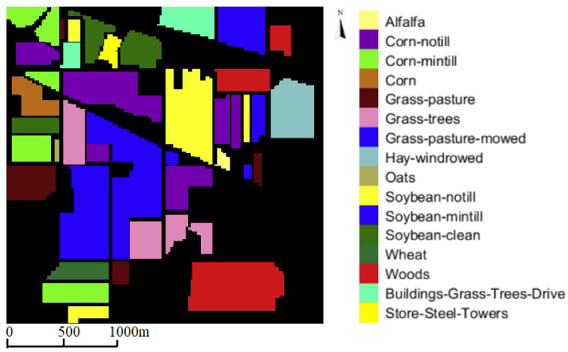
In the experiment, two datasets with different characteristics, i.e., the Indian Pines dataset (Indian Pines) and the Pavia Center dataset (Pavia), were selected. Indian pines were acquired on 12 June 1992 at the Purdue University Agricultural College in northwestern West Lafayette with an airborne visible/infrared imaging spectrometer (AVIRIS) sensor system with $145\times 145$ pixels. After removing the noise, the image contains 200 spectral information bands with a resolution of 20 m. There are 16 real objects with labels in the image [30], as shown in Figure 5.

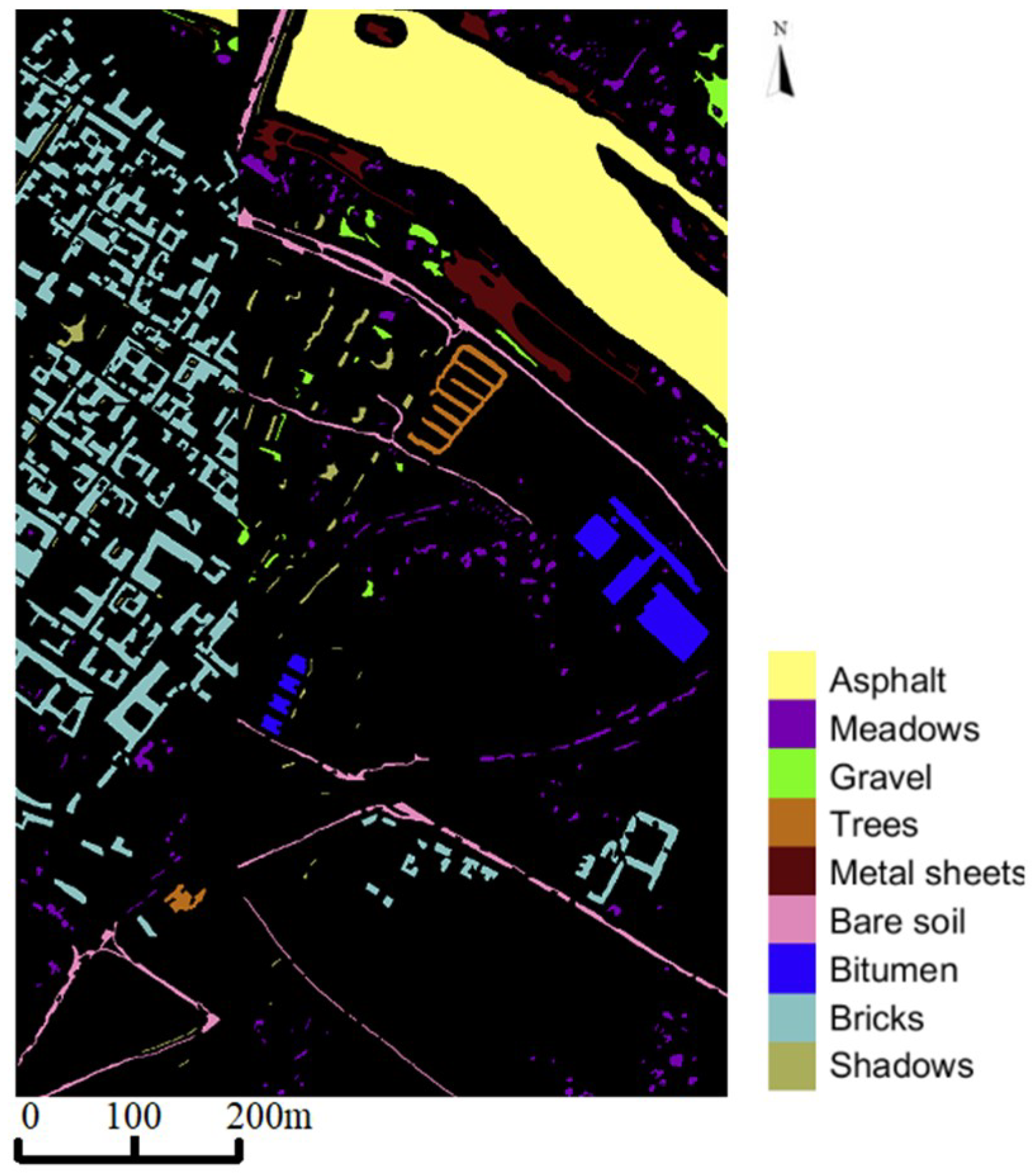
PaviaC was obtained through the Reflex Optical System Imaging Spectrometer hyperspectral sensor system in the city center near Pavia University in Pavia, northern Italy. After removing the noise, the data contain $1096\times 175$ pixels. The image has a resolution of 1.3 m and a total of 102 spectral bands. This image contains 9 types of objects [31], as shown in Figure 6.

In these experiments, under-segmentation error (UE), achievable segmentation accuracy (ASA), and boundary recovery (BR) were used to evaluate the performance of the proposed algorithm [32]. UE measures the fraction of pixel leakage across the truth boundaries of the ground. Smaller value of UE indicates the better performance. In ideal situations, the classification results are all correct, so the calculation result of UE is 0. BR estimates the percentage of true natural boundaries recovered by segmentation of superpixel boundaries. In ideal situations, the superpixel boundaries are the same as real boundaries and the calculation result of BR is 1. A larger value of BR indicates the better segmentation performance. Complete accurate segmentation rate (ASA) measures the upper bound of the performance. ASA represents the highest precision of segmentation in superpixels. A larger ASA indicates the better performance. In the ideal situation, the result of ASA is 1.

In this paper, we implemented the generation of false color images on the platform of MatLAB2014a, and implemented the hyperpixel segmentation of hyperspectral images on the platform of VS2008 with the extended Opencv library. The specific experimental design is described as follows.

4.1. Parameters Selection Experiments

In this section, the results and discussions may be presented in separate subsections or in one combined subsection.

IM-CHD algorithm has three key parameters, i.e., the number of selected spectral bands $n$, the window size $m$, and the third is the threshold $\sigma$. The three parameters need to be adjusted manually. The three key parameters decide the exclusion of spectral bands and have a great influence on the dimensionality of HSIs.

4.1.1. Number of Selected Bands

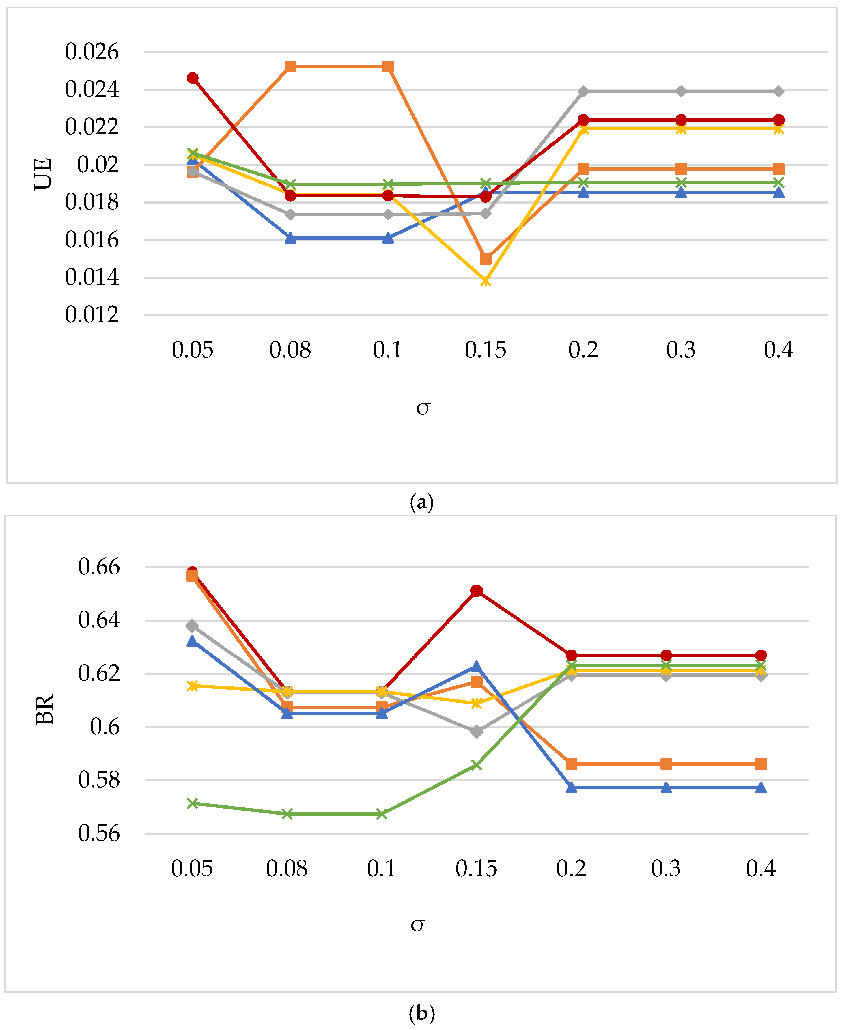
First of all, the number of selected bands was set to $n=1,2,3,4,5,8,10$. When $n>10$, more than 30 spectral bands would be selected, which makes dimensionality reduction meaningless. The window size was set to $m=11$, while the value of $\sigma$ varied. Using the dataset of Indian Pines, the effects of the number of selected spectral bands on UE, BR, ASA are shown in Figure 7. The polylines in different colors represent different numbers of selected spectral bands. For example, the red polyline represents the values of UE at $n=1$ and varying values of $\sigma$.

Figure 7a shows the results of UE at different values of $n$ and $\sigma$. From Figure 7a, when $n=1$ and $\sigma$ were set to different values, the obtained UE in red polyline was mostly the smallest, indicating the better performance result at $n=1$.

Figure 7b shows the BR results at different values of $n$ and $\sigma$. The red polyline represents the BR values at $n=1$, that is, the experimental results when only three spectral bands were selected. From the figure, when $n=1$, the obtained polyline (red) was always above other polylines at any value of $\sigma$. Therefore, when $n=1$, the value of BR was the largest, and the obtained segmented image had the best performance.

Figure 7c shows the ASA results at different values of $n$ and $\sigma$. When $\sigma =0.05$, the red line is at the highest point and the value of ASA is the largest. Meanwhile, the red line is more stable than the orange line. Therefore, when $n=1$, the best segmentation results can be obtained.

From the results, when $n=1$, UE was relatively low, BR and ASA were relatively high. At $n=1$, the segmentation results were more satisfactory than the results at other values of $n$. When $n=1$, three least relevant spectral bands were selected, and they contained the largest amount of information and minimum redundancy. Therefore, when the value of the parameter $n$ was 1, the performance was optimal.

4.1.2. Threshold Parameter $\sigma$

Based on information measures, the threshold parameter $\sigma$ has a great influence on the dimensionality of HSIs. In the experiment, three bands ($n=1$) were selected and the window size was set to $m=11$. Using the dataset of Indian Pines, the influences of the threshold $\sigma$ on UE, BR, ASA are shown in

Table 1. Superpixel segmentation performance under different $\sigma$ ($m=11$) on Indian Pines.

$\mathit{\sigma }$	0.05	0.1	0.15	0.2	0.3	0.4
UE	0.0203	0.0161	0.0149	0.0185	0.0185	0.0185
BR	0.6580	0.6132	0.6511	0.6268	0.6268	0.6268
ASA	0.8655	0.8408	0.8491	0.8350	0.8350	0.8350

.

It is important to choose the appropriate window size $m$ and threshold $\sigma$. According to Table 1, when $\sigma =0.15$, the UE had the lowest. However, BR and ASA were relatively low. When $m=11$, $\sigma \ge 0.2$ ($\sigma =0.2$, $\sigma =0.3$, $\sigma =0.4$), the values of ASA, UE, and BR were the same. The results indicated when $\sigma$ is large enough, the impact of different thresholds on the segmentation result is almost the same. When $\sigma =0.05$, the values of BR and ASA reached the maximum simultaneously. The three indicators were considered comprehensively to evaluate the performance of segmentation. Thus, when BR and ASA were simultaneously maximal, even if UE was a bit high, it still can be considered that the segmentation performance at $\sigma =0.05$ was more satisfactory. In the following experiments, the value of $\sigma$ was set to 0.05.

4.1.3. Window Size $m$

The window size $m$ has a great influence on the dimensionality of HSIs based on information measures. In the experiment, three bands ($n=1$) were selected and the threshold was set to $\sigma =0.1$. Using the dataset of Indian Pines, the effects of different window size $m$ on UE, BR, ASA are shown in

Table 2. Superpixel segmentation performance under different values of $m$ ($\sigma =0.05$) on Indian Pines.

$\mathit{m}$	5	9	11	14	17	20
UE	0.0149	0.0156	0.0203	0.0203	0.0179	0.0203
BR	0.6511	0.6470	0.6580	0.6580	0.6580	0.6610
ASA	0.8491	0.8661	0.8408	0.8655	0.8655	0.8650

.

As shown in Figure 1, in the image of “Indian pines”, the curvature changed steeply, thus selecting a large window size $m$ and a moderate $\sigma$ was more suitable. In addition, from Table 2, the experimental results showed that when $m=20$, $\sigma =0.05$, the experimental results of the segmentation were optimal. Under this condition, both BR and ASA were high, even though UE was a little high, the segmentation performance was still considered to be satisfactory. Through the above two parameter selection experiments, the most suitable values for the experimental parameters can be determined in the comparison experiment.

4.2. Comparison Experiments

In this section, the performance of the proposed IM-CHD algorithm was compared with similar existing algorithms. At first, the IM-CHD was compared with the conventional image color visualization method [21] based on information measures (CV-CHD). Then the proposed IM-CHD was compared to six other combined algorithms. Specifically, the conventional first principal component (FPC) extraction algorithm [33] and principal component (PC) weighted false color composition (FCC) algorithm [19] were combined with the conventional SLIC algorithm [16], new LSC algorithm [34], and the CHD superpixel segmentation algorithm [19] to obtain the 6 combined algorithms, i.e., FPC based SLIC (FPC-SLIC), FPC based LSC (FPC-LSC), FPC based CHD SS (FPC-CHD), FCC based SLIC (FCC-SLIC), FCC based LSC (FCC-LSC), FCC based CHD (FCC-CHD). In the experiments, the number of iterations, Niter, was set to 10, the PC threshold was set to $\mathrm{T}=0.99$, and the distance weight coefficient was set to $\mu =1$. In IM-CHD method, the parameters were set as follows: $n=1$, $m=20$ and $\sigma =0.05$.

4.2.1. Experiment Using Indian Pines Dataset

First, the comparison experiments were performed on the Indian Pines dataset. The obtained experimental results are shown in Figure 8 and

Table 3. Superpixel segmentation performance under different methods on Indian Pines.

Different Methods	FPC-SLIC	FCC-SLIC	FPC-LSC	FCC-LSC	FPC-CHD	FCC-CHD	CV-CHD	IM-CHD
UE	0.0312	0.0276	0.0286	0.0311	0.0211	0.0187	0.0162	0.0149
BR	0.3415	0.3385	0.4873	0.4502	0.6378	0.6434	0.6026	0.6511
ASA	0.8241	0.8186	0.8505	0.8447	0.8628	0.8666	0.8524	0.8491

. In the experiment, the obtained results were averaged by ten times.

Figure 8a shows the results of parameter UE using 8 algorithms. The smaller value of the UE indicated the smaller error and the better the segmentation performance. From the figure, the UE value using CV-CHD and IM-CHD is obviously lower than that using the other six algorithms. In details, from Table 3, compared with FCC-CHD, the error rate of IM-CHD(UE) was reduced by more than 15%; compared with CV-CHD, the error rate of IM-CHD(UE) was reduced by more than 8%.

Figure 8b shows the results of the parameter BR using eight algorithms. The larger value of BR indicated that the boundary obtained by superpixel segmentation was closer to the natural boundary. From the results, CV-CHD and IM-CHD were superior to FPC-CHD and FCC-CHD. In addition, all the above four algorithms (CV-CHD, IM-CHD, FPC-CHD, and FCC-CHD) were much better than the other algorithms. From Table 3, compared with FCC-CHD, the missed boundaries in the IM-CHD algorithm were reduced by more than 5%. Compared with CV-CHD, the missed boundaries were reduced by 8%.

Figure 8c shows the results of the parameter ASA using eight algorithms. The larger ASA value indicated higher accuracy of the segmentation result. From the figure, the obtained ASA values using different methods were relatively stable. Based on ASA, CV-CHD, IM-CHD, FCC-CHD, and FPC-CHD had relatively better performance. The segmentation accuracy of CV-CHD was similar to that of FCC-CHD. The ASA value of IM-CHD was slightly lower. But compared with the maximum ASA value obtained by the FCC-CHD method, the ASA value of IM-CHD was reduced by less than 2%.

By comprehensively considering the values of the three evaluation indicators, it can be concluded that the segmentation results obtained by the IM-CHD method are the best.

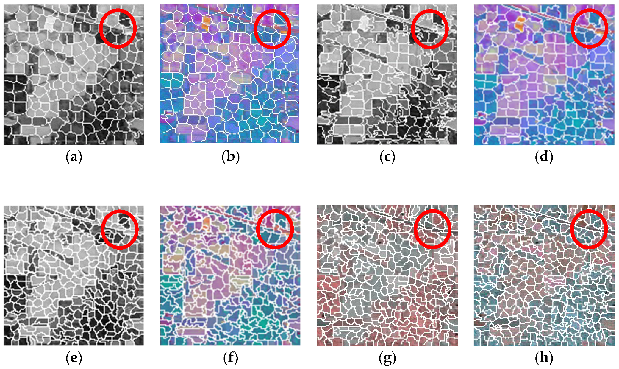
Figure 9 shows the segmentation results of the Indian Pines dataset under different segmentation methods. Under the same number of iterations, the number of superpixels obtained by different algorithms was different. More obtained superpixels indicated that the segment algorithm was more efficient. From the results, the IM-CHD method can better capture the boundary information and can allocate more superpixels to represent complex areas.

In the three methods, i.e., FPC-SLIC, FPC-LSC, and FPC-CHD, the images were segmented according to the first principal component map of the HSIS. Therefore, the obtained colors using these three methods were slightly different from the other five methods.

From Figure 9, the superpixel results using different segmentation methods were slightly different. The CV-CHD and IM-CHD methods can better segment the real boundaries of ground objects, such as areas within a red circle. In both algorithms, more superpixel blocks were assigned to represent the regions with complex colors while fewer superpixels were used for the regions with simple colors. Therefore, more precise results can be obtained using both CV-CHD and IM-CHD.

4.2.2. Experiment Using PaviaC Dataset

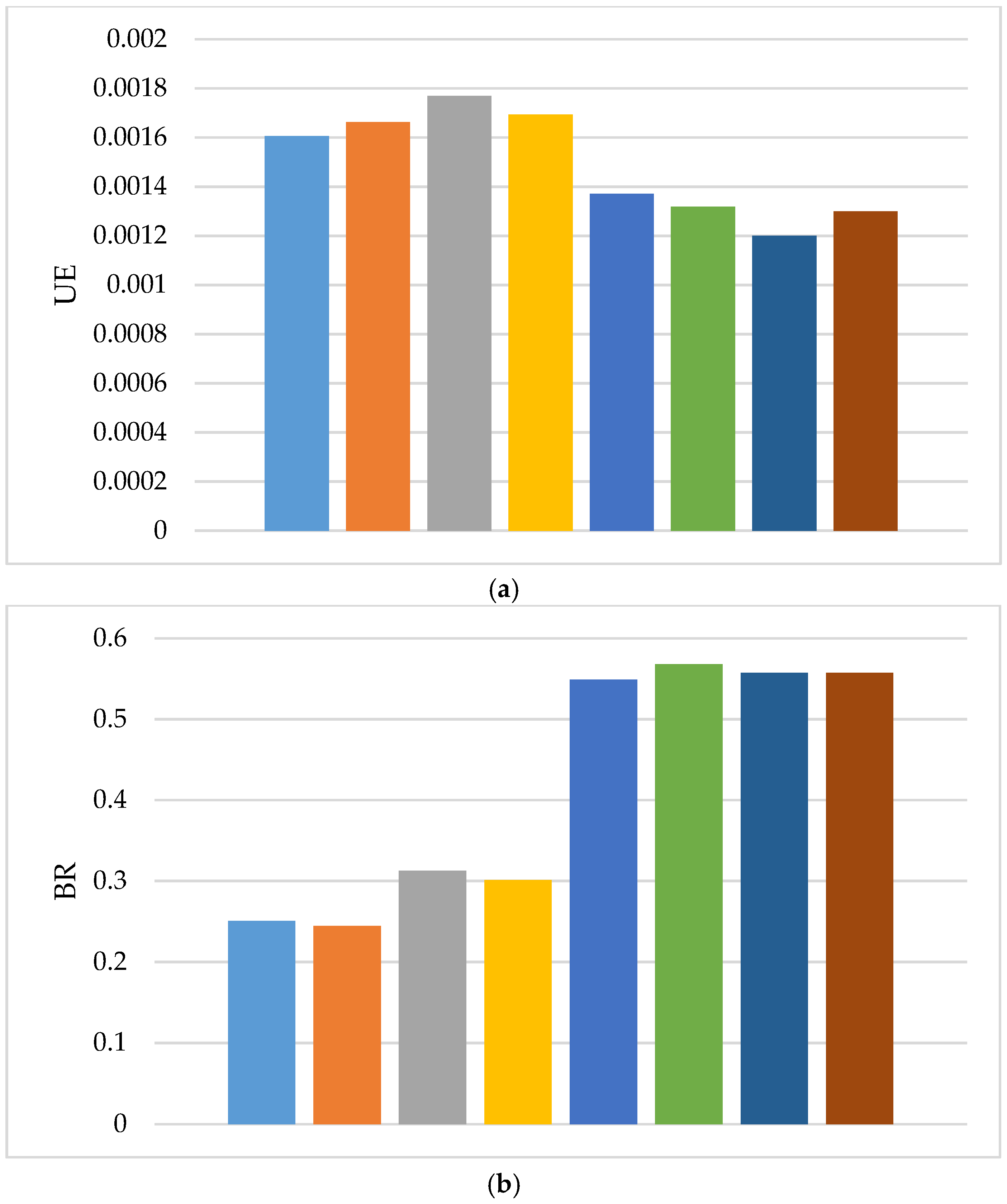
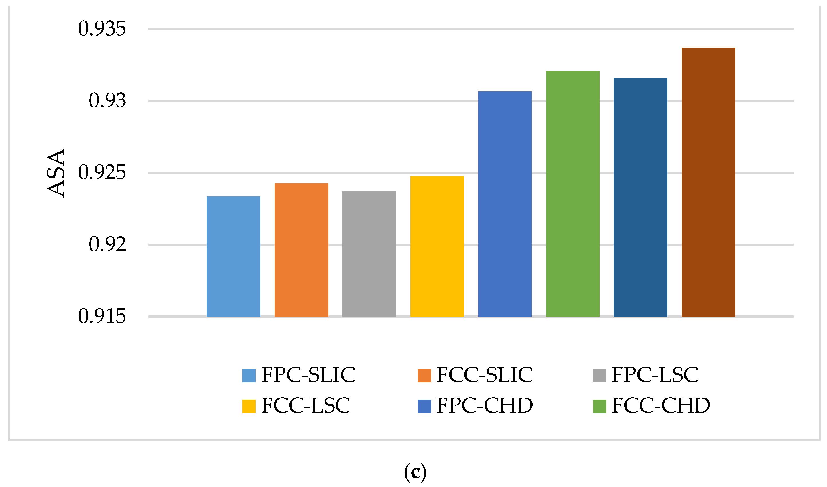
Figure 10 and

Table 4. Superpixel segmentation performance using different methods on PaviaC.

Different Methods	FPC-SLIC	FCC-SLIC	FPC-LSC	FCC-LSC	FPC-CHD	FCC-CHD	CV-CHD	IM-CHD
UE	0.0016	0.0016	0.0017	0.0016	0.0013	0.0013	0.0012	0.0013
BR	0.2507	0.2444	0.3127	0.3010	0.5487	0.5678	0.5572	0.5574
ASA	0.9233	0.9242	0.9237	0.9247	0.9306	0.9320	0.9315	0.9336

show the experimental results on the PaviaC dataset. Figure 10 shows the best results generated by each method. Table 4 shows the detailed experimental results.

Figure 10a shows the results of the parameter UE using 8 algorithms. The histogram height of UE using IM-CHD and CV-CHD was lower than using the other six algorithms. From Table 4, the obtained value UE using IM-CHD was the same as using FCC-CHD and FPC-CHD. Therefore, IM-CHD method had the second best UE performance (CV-CHD method resulted in the lowest UE value).

Figure 10b shows the results of the parameter BR using eight algorithms. FCC-CHD, FPC-CHD, CV-CHD, and IM-CHD were superior to FFC-LSC and FPC-LSC, while the above six algorithms were much better than FCC-SLIC and FPC-SLIC. From Table 4, among all the eight methods, IM-CHD method provided the second largest BR value.

Figure 10c shows the results of the parameter ASA using eight algorithms. IM-CHD was superior to all the other seven methods, i.e., FFC- FCC-CHD, FPC-CHD, FFC-LSC, FPCLSC, FFC-SLIC, FPC-SLIC, and CV-CHD. In Table 4, compared to CV-CHD, the ASA value obtained by IM-CHD was increased by 0.2%. Therefore, based on ASA, IM-CHD exhibited the best performance.

Among all the segmentation methods of this experiment, according to the comprehensive consideration of the three evaluation indicators, our proposed IM-CHD method had the best performance and the highest classification accuracy.

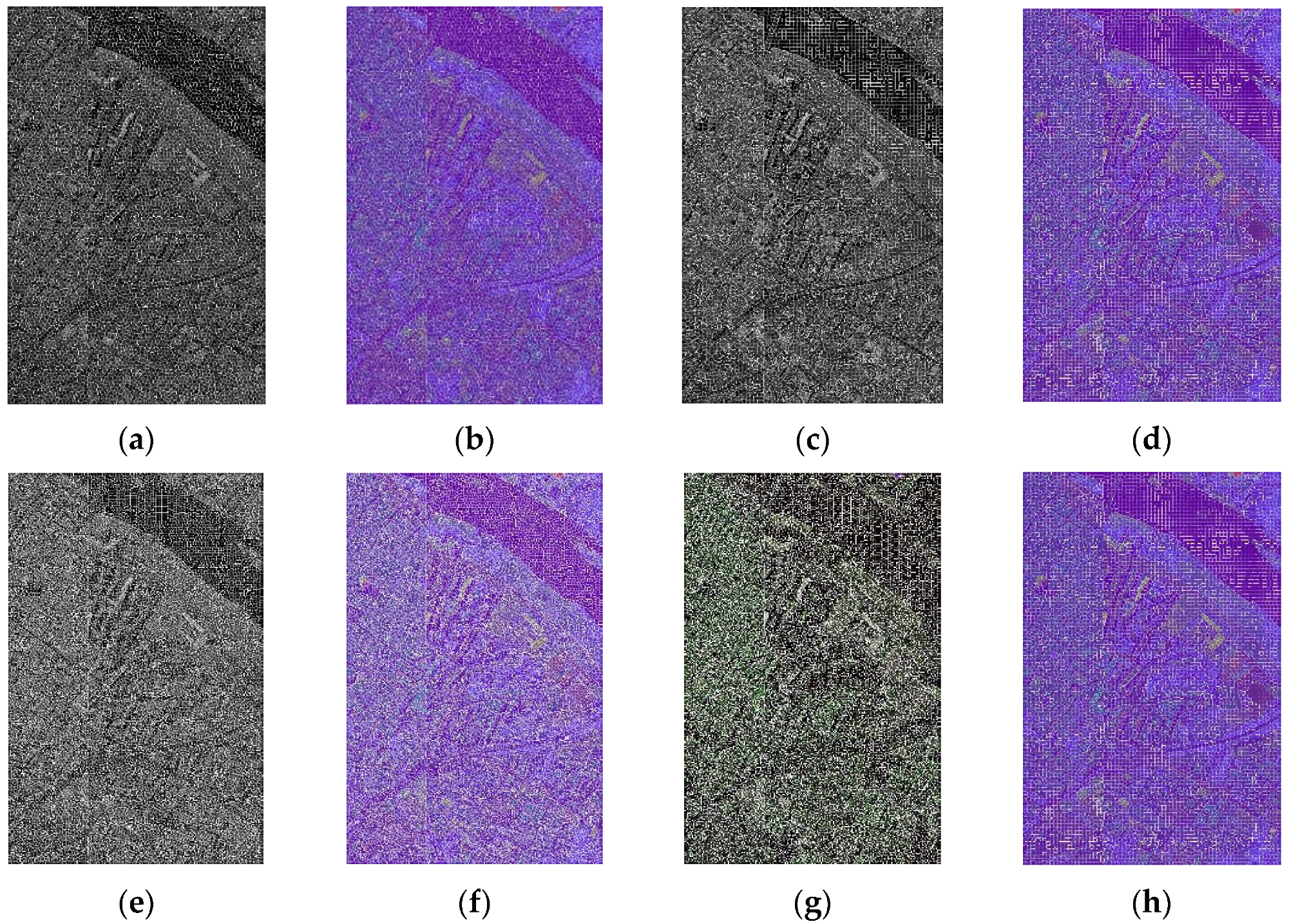
Figure 11 shows the example segmentation results on PaviaC dataset. Due to the same reason as in Figure 9, the segmentation result pictures using different methods had different colors.

From Figure 11, using IM-CHD, the density of the obtained superpixel blocks is more reasonable, which is consistent with the observations from Figure 9.

By comprehensively analyzing the performance of eight algorithms on Indian Pines and PaviaC datasets, it can be concluded that the segmentation results obtained by IM-CHD are more reasonable and accurate. The experiment results proved the effectiveness of the proposed method.

5. Conclusions

In this paper, first, the superpixel segmentation algorithm based on information measures with color histogram driving was introduced. The spectral bands were selected based on entropy and CMF. In these selected bands, the redundant information was removed while the significant information was retained for further superpixel segmentation. Then, the mutual information was used to select the final three groups of bands, i.e., $3n$ bands, to composite false color images. The smaller value of the mutual information indicated the less redundancy between the spectral bands and the greater amount of contained information. In our study, the segmentation results were obtained using the hill climbing optimization algorithm. In addition, parameter selection experiments and comparative experiments were designed and implemented in this study. Under the optimal parameter, the proposed IM-CHD was compared with other similar existing methods. The experimental results demonstrated the effectiveness and superiority of the proposed IM-CHD method. Therefore, the proposed method achieved the purpose of efficient preprocessing of hyperspectral images.

Previously, we proved the validity of obtaining the main spectra of HSIs through information measure. In the future, we will study the application of superpixel segmentation based on information measurement in the classification of hyperspectral images. That is, the IM-CHD method proposed in this paper is used to preprocess HSIs and classify the processed HSIs. The classification results are compared with the previously proposed HSIs classification method, and it is discussed whether IM-CHD method can improve the classification accuracy of HSIs.

References

1. Fauvel, M.; Tarabalka, Y.; Benediktsson, J.A.; Chanussot, J.; Tilton, J.C. Advances in spectral-spatial classification of hyperspectral images. Proc. IEEE 2012, 101, 652–675. [Google Scholar] [CrossRef] [Green Version]
2. Yang, H.; Du, Q.; Su, H.; Sheng, Y. An efficient method for supervised hyperspectral band selection. IEEE Geosci. Remote Sens. Lett. 2010, 8, 138–142. [Google Scholar] [CrossRef]
3. Martínez-Usó, A.; Pla, F.; García-Sevilla, P. Automatic band selection in multispectral images using mutual information-based clustering. In Proceedings of the Iberoamerican Congress on Pattern Recognition, Cancun, Mexico, 14–17 November 2006; pp. 644–654. [Google Scholar]
4. Wang, B.; Wang, X.; Chen, Z. Spatial mutual information based hyperspectral band selection for classification. Sci. World J. 2015, 2015. [Google Scholar] [CrossRef] [Green Version]
5. Kwarteng, P.; Chavez, A. Extracting spectral contrast in Landsat Thematic Mapper image data using selective principal component analysis. Photogramm. Eng. Remote Sens. 1989, 55, 339–348. [Google Scholar]
6. Wang, L.; Jia, X.P.; Zhang, Y. A novel geometry-based feature-selection technique for hyperspectral imagery. IEEE Geosci. Remote Sens. Lett. 2007, 4, 171–175. [Google Scholar] [CrossRef]
7. Chen, Y.; Nasrabadi, N.M.; Tran, T.D. Sparsity-based classification of hyperspectral imagery. Geosci. Remote Sens. Symp. IEEE 2010. [Google Scholar] [CrossRef]
8. Jacobson, N.P.; Gupta, M.R. Design goals and solutions for display of hyperspectral images. IEEE Trans. Geosci. Remote Sens. 2005, 43, 2684–2692. [Google Scholar] [CrossRef]
9. Acito, N.; Corsini, G.; Diani, M. An unsupervised algorithm for hyperspectral image segmentation based on the Gaussian mixture model. In Proceedings of the IEEE International Geoscience and Remote Sensing Symposium, Toulouse, France, 21–25 July 2003. [Google Scholar] [CrossRef]
10. Veganzones, M.A.; Tochon, G.; Dalla-Mura, M.; Plaza, A.J.; Chanussot, J. Hyperspectral image segmentation using a new spectral unmixing-based binary partition tree representation. IEEE Trans. Image Process. 2014, 23, 74–89. [Google Scholar] [CrossRef] [PubMed]
11. Rundo, L.; Tangherloni, A.; Cazzaniga, P.; Nobile, M.S.; Russo, G.; Gilardi, M.C.; Militello, C.; Vitabile, S.; Mauri, G.; Besozzi, D. A novel framework for MR image segmentation and quantification by using MedGA. Comput. Methods Programs Biomed. 2019, 176, 159–172. [Google Scholar] [CrossRef] [PubMed]
12. Jiayin, L.; Zhenmin, T.; Ying, C.; Guoxing, W. Local competition-based superpixel segmentation algorithm in remote sensing. Sensors 2017, 17. [Google Scholar] [CrossRef]
13. Ren, X.; Malik, J. Learning a classification model for segmentation. ICCV 2003, 1, 10–17. [Google Scholar] [CrossRef] [Green Version]
14. Liu, M.Y.; Tuzel, O.; Ramalingam, S.; Chellappa, S. Entropy rate superpixel segmentation. Comput. Vis. Pattern Recognit. 2011. [Google Scholar] [CrossRef]
15. Bergh, M.V.D.; Boix, X.; Roig, G.; Capitani, B.D.; Gool, L.V. SEEDS: Superpixels Extracted via Energy-Driven Sampling. In European Conference on Computer Vision; Springer: Berlin/Heidelberg, Germany, 2012. [Google Scholar] [CrossRef] [Green Version]
16. Zhang, X.; Chew, S.E.; Xu, Z.; Cahill, N.D. SLIC superpixels for efficient graph-based dimensionality reduction of hyperspectral imagery. SPIE 2015. [Google Scholar] [CrossRef]
17. Xu, Q.; Fu, P.; Sun, Q.; Wang, T. A Fast Region Growing Based Superpixel Segmentation for Hyperspectral Image Classification. In Proceedings of the Chinese Conference on Pattern Recognition and Computer Vision (PRCV); Springer: Cham, Switzerland, 2019. [Google Scholar] [CrossRef]
18. Rundo, L.; Militello, C.; Vitabile, S.; Casarino, C.; Russo, G.; Midiri, M.; Gilardi, M.C. Combining split-and-merge and multi-seed region growing algorithms for uterine fibroid segmentation in MRgFUS treatments. Med. Biol. Eng. Comput. 2016, 54, 1071–1084. [Google Scholar] [CrossRef] [PubMed]
19. Rodarmel, C.; Shan, J. Principal component analysis for hyperspectral image classification. Salis 2002, 62, 115–122. [Google Scholar]
20. Zhang, Y.; Jiang, X.; Wang, X.; Cai, Z. Spectral-Spatial Hyperspectral Image Classification with Superpixel Pattern and Extreme Learning Machine. Remote Sens. 2019, 11, 1983. [Google Scholar] [CrossRef] [Green Version]
21. Le Moan, S.; Mansouri, A.; Voisin, Y.; Hardeberg, J.Y. A constrained band selection method based on information measures for spectral image color visualization. IEEE Trans. Geosci. Remote Sens. 2011, 49, 5104–5115. [Google Scholar] [CrossRef] [Green Version]
22. Lin, L.; Chen, C.; Yang, J.; Zhang, S. Deep Transfer HSI Classification Method Based on Information Measure and Optimal Neighborhood Noise Reduction. Electronics 2019, 8, 1112. [Google Scholar] [CrossRef] [Green Version]
23. David, L. Hyperspectral image data analysis as a high dimensional signal processing problem. IEEE Signal Process. Mag. 2002, 19, 17–28. [Google Scholar]
24. Shannon, C.E. A mathematical theory of communication. Bell Labs Tech. J. 1948, 27, 379–423. [Google Scholar] [CrossRef] [Green Version]
25. Bell, A.J. The co-information lattice. In Proceedings of the 5th International Workshop on Independent Component Analysis and Blind Signal Separation: ICA. April 2003. Available online:https://pdfs.semanticscholar.org/25a0/cd8d486d5ffd204485685226f189e6eadd4d.pdf (accessed on 12 February 2020).
26. Shaw, M.Q.; Fairchild, M.D. Evaluating the 1931 CIE Color Matching Functions. Proc. AIC 2001, 316–329. [Google Scholar] [CrossRef]
27. Martinez-Uso, A.; Pla, F.; Sotoca, J.M.; Sevilla, P.G. Clustering-based hyperspectral band selection using information measures. IEEE Trans. Geosci. Remote Sens. 2008, 45, 4158–4171. [Google Scholar] [CrossRef]
28. Lin, L.; Yang, J.; Zhou, Z. Superpixel segmentation for hyperspectral images based on false color composition with color histogram driving. Int. J. Remote Sens. 2018, 307–331. [Google Scholar] [CrossRef]
29. Masra, S.M.W.; Pang, P.K.; Muhammad, M.S.; Kipli, K. Application of particle swarm optimization in histogram equalization for image enhancement. In Proceedings of the Humanities, Science and Engineering (CHUSER), Kota Kinabalu, Malaysia, 3–4 December 2012. [Google Scholar] [CrossRef] [Green Version]
30. Camps-Valls, G.; Bandos Marsheva, T.; Zhou, D. Semi-supervised graph-based hyperspectral image classification. IEEE Trans. Geosci. Remote Sens. 2007, 45, 3044–3054. [Google Scholar] [CrossRef]
31. Palmason, J.A.; Benediktsson, J.A.; Sveinsson, J.R.; Chanussot, J. Classification of hyperspectral data from urban areas using morphological preprocessing and independent component analysis. In Proceedings of the 2005 IEEE International Geoscience and Remote Sensing Symposium, Seoul, Korea, 29–29 July 2005. [Google Scholar] [CrossRef]
32. Veksler, O.; Boykov, Y.; Mehrani, P. Superpixels and Supervoxels in an Energy Optimization Framework. In Proceedings of the Computer Vision—ECCV 2010—11th European Conference on Computer Vision, Heraklion, Crete, Greece, 5–11 September 2010. [Google Scholar] [CrossRef] [Green Version]
33. David, W.; Dunteman, G.H. Principal Components Analysis. 1990. Available online:https://books.google.com.ph/books?hl=zh-CN&lr=&id=Pzwt-CMMt4UC&oi=fnd&pg=PA5&dq=Principal+Components+Analysis&ots=igfoyzhMg1&sig=QceIG76XG1r3HJ7mzvAC_s22gw8&redir_esc=y#v=onepage&q=Principal%20Components%20Analysis&f=false (accessed on 12 February 2020).
34. Chen, J.; Li, Z.; Huang, B. Linear Spectral Clustering Superpixel. IEEE Trans. Image Process. 2017, 26, 3317–3330. [Google Scholar] [CrossRef] [PubMed]
Figure 1. Entropy (blue curve), local average (green curve) and thresholds (red curve) for the “Indian pines” image.
Applsci 10 01261 g001
Figure 2. The 1931 CIE color matching curves of the three primary colors of light (red, green, and blue) between 360 nm and 830 nm (at the interval of 5 nm)
Applsci 10 01261 g002
Figure 3. Red CMF (The horizontal lines represent two spectral thresholds in two cases. The spectral band is retained when the CMF coefficient is above the threshold.).
Applsci 10 01261 g003
Figure 4. Flow chart of superpixel segmentation for hyperspectral images based on information measures.
Applsci 10 01261 g004
Figure 5. Ground truth of Indian Pines dataset.
Applsci 10 01261 g005
Figure 6. Ground truth of PaviaC dataset.
Applsci 10 01261 g006
Figure 7. The superpixel segmentation results at different values of n and window size m ( σ = 0.1 ) on Indian Pines: (a) UE; (b) BR; (c) ASA.
Applsci 10 01261 g007aApplsci 10 01261 g007b
Figure 8. The superpixel segmentation results of different methods on Indian Pines: (a) UE; (b) BR; (c) ASA.
Applsci 10 01261 g008
Figure 9. The superpixel segmentation images using different methods on Indian Pines dataset: (a) FPC-SLIC; (b) FCC-SLIC;(c) FPC-LSC;(d) FCC-LSC; (e) FPC-CHD; (f) FCC-CHD; (g) CV-CHD; (h) IM-CHD.
Applsci 10 01261 g009
Figure 10. The superpixel segmentation results using different methods on PaviaC dataset. (a) UE; (b) BR; (c) ASA.
Applsci 10 01261 g010aApplsci 10 01261 g010b
Figure 11. The superpixel segmentation images of different methods on PaviaC dataset: (a) FPC-SLIC; (b) FCC-SLIC; (c) FPC-LSC; (d) FCC-LSC; (e) FPC-CHD; (f) FCC-CHD; (g) CV-CHD; (h) IM-CHD.
Applsci 10 01261 g011