Autonomous Underwater Vehicles: Localization, Navigation, and Communication for Collaborative Missions

Abstract

Development of Autonomous Underwater Vehicles (AUVs) has permitted the automatization of many tasks originally achieved with manned vehicles in underwater environments. Teams of AUVs designed to work within a common mission are opening the possibilities for new and more complex applications. In underwater environments, communication, localization, and navigation of AUVs are considered challenges due to the impossibility of relying on radio communications and global positioning systems. For a long time, acoustic systems have been the main approach for solving these challenges. However, they present their own shortcomings, which are more relevant for AUV teams. As a result, researchers have explored different alternatives. To summarize and analyze these alternatives, a review of the literature is presented in this paper. Finally, a summary of collaborative AUV teams and missions is also included, with the aim of analyzing their applicability, advantages, and limitations.

1. Introduction

Over the years, a large number of AUVs are being designed to accomplish a wide range of applications in the scientist, commercial, and military areas. For oceanographic studies, AUVs have become very popular to explore, collect data, and to create 3D reconstructions or maps [1,2]. At the oil and gas industry, AUVs inspect and repair submerged infrastructures and also have great potential in search, recognition, and localization tasks like airplane black-boxes recovery missions [3,4]. AUVs are also used for port and harbor security tasks such as environmental inspection, surveillance, detection and disposal of explosives and minehunting [5,6].

Design, construction, and control of AUVs represent such a challenging work for engineers who must face constraints they do not encounter in other environments. Above water, most autonomous systems rely on radio or spread-spectrum communications along with global positioning. In underwater environments, AUVs must rely on acoustic-based sensors and communication. Design and implementation of new technologies and algorithms for navigation and localization of AUVs—especially for collaborative work—is a great research opportunity.

Before establishing a collaborative scheme for AUVs, the problem of localization and navigation must be addressed for every vehicle in the team. Traditional methods include Dead-Reckoning (DR) and Inertial Navigation Systems (INS) [7]. DR and INS are some of the earliest established methods to locate an AUV [8]. These systems rely on measurements of the water-speed and the vehicle’s velocities and accelerations that, upon integration, leads to the AUV position. They are suitable for long-range missions and have the advantage to be passive methods—they do not need either to send or receive signals from external systems—resulting in a solution immune to interferences. Nevertheless, the main problem of them is that the position error growths over time—which is commonly known as accuracy drift—as a result of different factors such as the ocean currents and the accuracy of the sensors itself, which are not capable of sensing the displacements produced by external forces or the effects of earth’s gravity. The use of geophysical maps to matching the sensors measurements is an alternative to deal with the accuracy drifts of the inertial systems. This method is known as Geophysical Navigation (GN) [9] and allows accomplishing longer missions maintaining a position error relatively low. However, there is a need for having the geophysical maps available before the mission, which is one the main disadvantages of GN along with the computational cost of comparing and matching the map with the sensors data. Acoustic ranging systems have been another common alternative for AUV navigation [10]. These systems can be implemented using acoustic transponders to locate an AUV in either global or relative coordinates. However, most of them require complex infrastructure and the cost of such deployments could be higher compared with other methods. In recent years, researchers are exploring new alternatives for AUV localization and navigation. Optical technologies have become very popular for robots and vehicles at land or air environments [11], but face tough conditions in underwater environments that have delayed the development of such technologies for AUVs. When the underwater conditions permit a proper light propagation and detection, visual-based systems can improve significantly the accuracy of the position estimations and reach higher data rates that acoustic systems. Finally, recent advancements in terms of sensor fusion schemes and algorithms are contributing to the development of hybrid navigation systems, which takes the advantages of different solutions to overcome their weaknesses. A sensor fusion module improves the AUV state estimation by processing and merging the available sensors data [12]. Some of the common sensors used for it are the inertial sensors of an INS, Doppler Velocity Loggers (DVL), and depth sensors. Recently, the INS measurements are also being integrated with acoustic/vision-based systems to produce a solution that, beyond reducing the accuracy drifts of the INS, will have high positioning accuracy in short-ranges. All these technologies are addressed in Section 2 of this work, which is organized as shown in Figure 1, including the main sensors used and the different approaches taken.

After solving the problem of self-localization and navigation, other challenges must be addressed to implement a collaborative team of AUVs. Since there is a need for sharing information between the vehicles, communication is an important concern. The amount and size of the messages will depend on the collaborative scheme used, the number of vehicles and the communication system capabilities. Acoustic-based performs better than light-based communication in terms of range, but not in data rates. It also suffers from many other shortcomings such as small bandwidth, high latency and unreliability [13]. Despite its notable merits in the terrestrial wireless network field, radio-based communication has had very few practical underwater applications to date [14]. The collaborative navigation scheme is also a mandatory issue to be considered. The underwater environment is complex by itself to navigate at, and now multiple vehicles have to navigate among each other. A proper formation has to ensure safe navigation for every single vehicle. These topics are analyzed in Section 3, which also includes a review on the main collaborative AUV mission: surveillance and intervention. Since there is no need to interact with the environment, survey missions are simpler to implement and have been performed successfully for different applications, such as mapping or object searching and tracking. Intervention missions are usually harder due to the complexity of the manipulators or actuators needed. In either case, since an experimental set up is difficult to be reached, many of the efforts made are being tested in simulation environments.

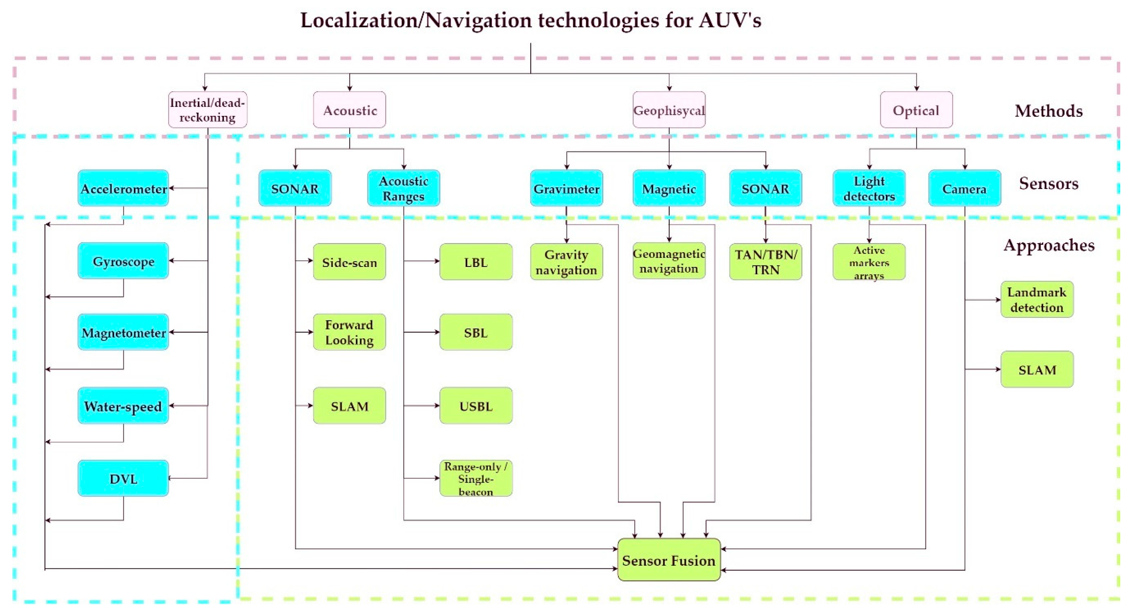
2. Navigation and Localization

Navigation and localization are two of the most important challenges for underwater robotics [11]. These continue being issues to solve for many applications such as collaborative missions. DR and INS are traditional methods for AUV localization and navigation but have issues as the decrement of the pose accuracy over time. In addition to traditional technologies, this problem was addressed in the past with acoustic technologies as Long Baseline (LBL) [15,16,17], Short Baseline (SBL) [18,19], or Ultra-Short Baseline (USBL) [20,21,22,23] systems. Acoustic positioning systems, though, require careful calibration of the sound velocity, as they suffer from multipath Doppler effects and susceptibility to thermoclines; they also have a limited range and accuracy [24]. Geophysical Navigation (GN) is also a solution for vehicle localization. Matching algorithms such as TERrain COntour-Matching (TERCOM) and Sandia Inertial Terrain Aided Navigation (SITAN) are relatively mature, however new algorithms are currently being proposed [25]. The main limitation of GN systems is the need for a geophysical map to compare the measurements from the sensors. Visual-based systems have been a trend for vehicle navigation at land and air environments, but there are several problems related to light propagation and detection in underwater environments. Additionally, most visual-based methods for autonomous navigation depend on the presence of features in the images taken, which, even if they exist, are difficult to extract due to the limited illumination conditions. In recent years, the field of AUV localization is shifting from old technologies, towards more dynamic approaches that require less infrastructure and offers a better performance [13]. This section presents a survey on single-vehicle localization and navigation technologies—including different methods, sensor, and approaches—in the understanding that those can be applied in multi-vehicle collaborative navigation schemes.

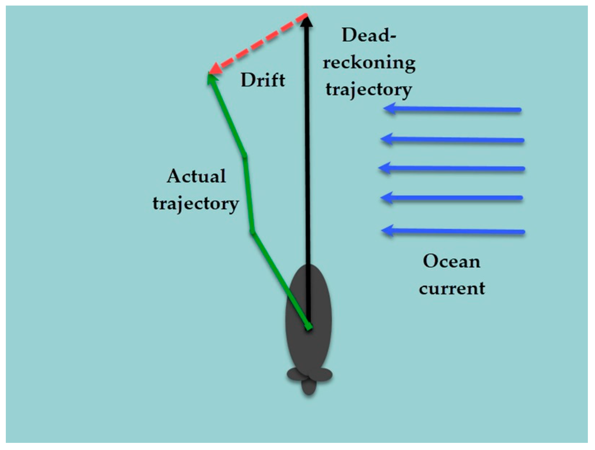
2.1. Dead-Reckoning and Inertial Navigation

The simplest method to obtain a position for a moving vehicle is by integrating its velocity in time. This method is known as dead-reckoning [8]. DR requires to know the velocity and direction of the vehicle, which is usually accomplished with a compass and a water speed sensor. The principal problem is related to the presence of an ocean current, as illustrated in Figure 2, because it will add a velocity component to the vehicle which is not detected by the speed sensor. Then, the accuracy of the method will be strongly affected especially when the vehicle navigates at a low velocity.

Inertial sensors can be used to improve the navigation accuracy and reliability of DR methods. The INS consist of three mutually-orthogonal accelerometers aligned to a gyroscopic reference frame. Measured accelerations are integrated to obtain the desired velocity, position, and attitude information of the vehicle. The fact that inertial navigation is self-contained—it neither emits nor receives any external signal—is one of its most significant strengths, making it a stealthy navigation solution, immune to interference or jamming [26]. However, the error on the pose estimations is known to increase over time, and depends on the accuracy of the sensors used. Mathematically, the total acceleration, denoted as $\ddot{r}$, can be expressed as follows [27]:

$$\ddot{r}=a+g,$$

(1)

where a is the acceleration calculated by the INS and g is the gravitational acceleration. Since the accelerometers do not sense the gravity, the position of the vehicle obtained by integrating the acceleration measurements will result with an error. Gyroscopic drifts are also a source of error that can result in significant misalignments between the sensor frame and the earth-fixed reference frame, causing navigation errors that also grows over time. Using a Global Positioning System (GPS) is a common method used to correct these errors. However, to correct the error accumulated by the INS, the vehicle must go to the surface to obtain a new GPS location at regular intervals, which can result in a waste of time and resources. Integration of an INS and a GPS data can also be a complex process, since those systems are based in completely different principles.

Even if the instruments were perfect, the estimations of an INS would result with an error [9]. The gyroscopic reference frame is aligned to a reference ellipsoid model of the earth. The reference ellipsoid conforms roughly to the shape of the earth, and in particular to mean sea level. If the mass of the earth were homogeneously distributed within the ellipsoid, the gravity vector would be normal to the reference ellipsoid surface. However, due to the inhomogeneous distribution of the earth mass, the gravity vector can have significant components tangential to the reference ellipsoid surface (known as vertical deflections) as shown in Figure 3. Since an INS cannot distinguish between the tangential components of earth gravity and the horizontal acceleration of the vehicle, these gravity disturbances cause errors in the INS velocity and position estimations.

The latest advances in MEMS inertial sensors are having profound effects on the recent availability of MEMS-Inertial Measurement Units (IMUs), that has become clearly attractive for a wide range of applications where size, weight, power, and cost are key considerations [28]. This set of sensors can be used to implement an Attitude and Heading Reference System (AHRS) or an INS. Some MEMS-based systems commercially available are showed in

Table 1. Commercial Inertial Measurement Unit (IMU)-Attitude and Heading Reference System (AHRS) systems

Manufacturer	Product Name	Heading Accuracy/ Resolution	Pitch and Roll Accuracy/ Resolution	Data Rate (Hz)	Depth Rated (m)
Impact Subsea	ISM3D [31]	±0.5°/0.1°	±0.07°/0.01°	250	1000–6000
Seascape Subsea	Seascape UW9XIMU-01 [32]	±0.5°/0.01°	±0.5°/0.01°	400	750
Inertial Labs	AHRS-10P [33]	±0.6°/0.01°	±0.08°/0.01°	200	600
SBG Systems	Ellipse2-N [34]	±1.0°/-	±0.1°/-	200	-
TMI-Orion	DSPRH [35]	±0.5°/0.1°	±0.5°/0.1°	100	500–2000
VectorNav	VN-100 [36]	±2.0°/0.05°	±1.0°/0.05°	400	-
XSENS	MTi-600 [37]	±1.0°/-	±0.2°/-	400	-

. Nevertheless, despite technological developments in inertial sensors, INS are underway to reduce the accuracy drift at the level of a few meters uncertainty over one hour of unaided inertial navigation [29]. Currently, damping techniques, using water speed measurements, are used to control velocity and position errors caused by uncorrected vertical deflection and inertial sensor errors [30]. However, this is at the cost of introducing an additional error source (the water-speed/ground-speed difference caused by ocean currents). Another alternative to reduce these effects is the use of maps of vertical deflection compensation values, as a function of latitude and longitude, to compensate the measured accelerations.

2.2. Acoustic Navigation

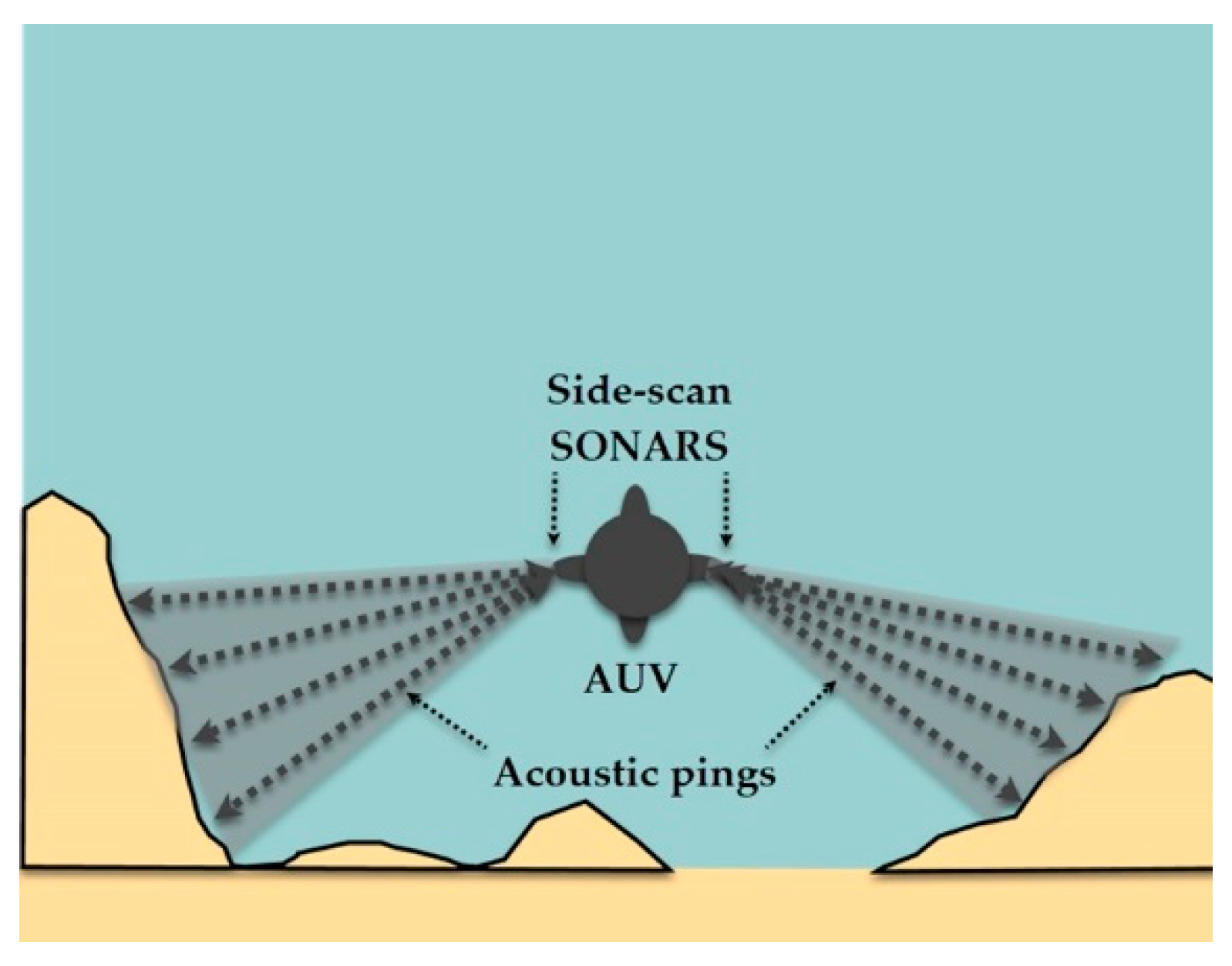
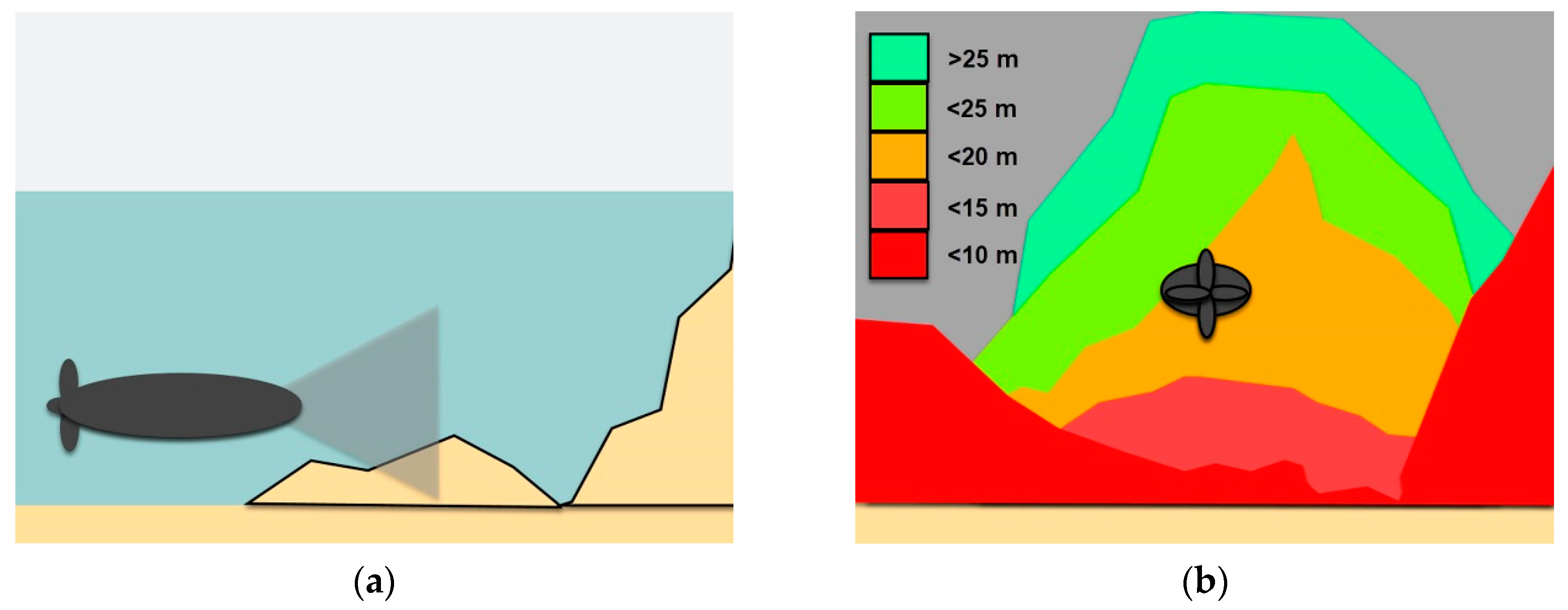
Compared with other signals, such radio and electromagnetic, acoustic-based signals propagates better in water and can reach considerable distances. This allows the use of acoustic transponders to navigate an AUV. Some of the navigation methods based on acoustic signals are the Sound Navigation and Ranging (SONAR), and acoustic ranging.

2.2.1. SONAR

There exist different methods to employ a SONAR for AUV navigation. Two basic configurations are the side-scan SONAR [10] and the Forward-Looking SONAR (FLS) [38]. Both of them are used to detect objects which can be: seabed changes, rocks, other vehicles, and even marine species. When an AUV is in operation, it must be able to detect these objects to update its navigation trajectory and avoid collisions, which is known as obstacle avoidance.

For the side-scan SONAR, the transducer device scans laterally when attached to the AUV, as illustrated in Figure 4. A series of acoustic pings are transmitted and then received, the time of the returns and the speed of sound in water is used to determine the existence of features located perpendicular to the direction of motion.

The FLS uses a searchlight approach, steering the sonar beam scanning forward of the vessel and streaming soundings on a continuous basis. FLS can be placed at different locations on the vehicle, as shown in Figure 5, to ensure that the AUV can detect obstacles from different directions.

Two-dimensional images can be produced which survey the ocean and the features on it. These images, while indicating what exists on the ocean or seafloor, do not contain localization information either relative or global.

Traditional obstacle avoidance planning methods include potential field, Bandler and Kohout (BK) products, particle swarm optimization, fuzzy controller, etc. Galarza et al. [39] designed an obstacle avoidance algorithm for an AUV. The obstacle detection system disposes of a SONAR and its use guarantees the safety of the AUV while navigating. Obstacle avoidance is performed based on a fuzzy reactive architecture for different forward speeds of the vehicle. The algorithm was validated under a computational simulation environment running in MATLAB. During the simulated route, the vehicle remained at a minimum distance of 5 m of the obstacles, reducing its reference forward speed of 1 m/s to values between 0.02 m/s and 0.4 m/s; thus, safe navigation around obstacles was achieved without losing the trajectory of navigation and reaching all the waypoints. Braginsky et al. [40] proposed an obstacle avoidance methodology based in the data collected from two FLS placed in horizontal and vertical orientation. FLS data is processed to provide obstacle detection information in the xz-and xy-planes, respectively. For the horizontal obstacle avoidance, authors used a two-layer algorithm. The first process of the algorithm is based on BK products of fuzzy relation, as a preplanning method; and the second is a reactive approach based on potential field and edge detection methods. In case that the horizontal approach fails finding a path to safely avoid the obstacle, a reactive vertical approach is activated. The sonar used in the experimentation has a detection range of up to 137 m and operated at a 450 kHz frequency. During the test, the mission definition for the AUV was to move from a starting point to a target point. Despite the maximum range of the FLS, decisions were made when an obstacle was within 40 m of the AUV. Lin et al. [41] implemented a Recurrent Neural Network (RNN) with Convolution (CRNN) for underwater obstacle avoidance. Offline training and testing were adopted to modify the neural network parameters of the AUV autonomous obstacle avoidance learning system, so self-learning is applied to the collision avoidance planning. Combining this learning system with FLS simulation data enables online autonomous obstacle avoidance planning in an unknown environment. Simulation results showed that the planning success rate was 98% and 99% for the proposed CRNN algorithms; meanwhile, it was 88% and 96% for the RNN algorithms. Authors concluded than the CRNN obstacle avoidance planner has the advantages of short training time, simple network structure, better generalization performance, and reliability than an RNN planner.

2.2.2. Acoustic Ranging

In acoustic ranging positioning systems, AUVs are equipped with an acoustic transmitter that establishes communication with a set of hydrophones. Knowing the propagation velocity of sound in underwater, the distance between the AUV and hydrophones can be calculated through the propagation time of the acoustic signal. Then, a location for the AUV with respect to the set of hydrophones can be obtained by geometric methods. One of the differences between acoustic systems is the arrangement of the hydrophones. In LBL systems, hydrophones are fixed within a structure or any other known underwater point of reference—known as landmark—[15]. The length of the baseline can be up to hundreds of meters. In SBL and USBL systems, the hydrophones are placed on buoys or another vehicle at the surface, even on a second AUV. For SBL systems, baseline length is measured in meters and works by measuring a relative position between the reference sound source and the receiving array; meanwhile, baseline for USBL systems is in decimeters and the relative location from the hydrophone to the moving target is calculated by measuring the phase differences between acoustic elements [18]. In either arrangement, hydrophones are generally located by Global Navigation Satellite Systems. In Figure 6, all three configurations for acoustic localization systems are shown.

A schematic diagram of an SBL system is represented in Figure 7. Three hydrophones, represented by H1, H2, and H3, are located at the points O, N, and M, at the origin of the reference frame and along the x and y axes, respectively. The distance from the detected vehicle to the i hydrophone is called oblique distance, which is denoted by D_i, with i = 1, 2, 3.

The vehicle receives a signal from a hydrophone (H1) and sends a reply that is received by all the hydrophones (H1, H2, and H3); then, signal run time is measured. The propagation time of the acoustic signal from the transmitter in the vehicle to the hydrophone base (T_i) is used to obtain the oblique distance with the equation [18]:

$$D_i=V · T_i,$$

(2)

where V is the nominal speed for underwater acoustic signals and is used as V = 1435 m/s. The location of the vehicle’s transmitter—point P—with coordinates X_p, Y_p, and Z_p, can be calculated using a traditional SBL model as follows:

$$P=\left(X_p,Y_p,Z_p\right)$$

(3)

$$X_p=\frac{D_1^2- D_2^2+N^2}{4N}$$

(4)

$$Y_p=\frac{D_1^2- D_3^2+M^2}{4M}$$

(5)

$$Z_P=\left\{{\left[D_1^2-X_p^2+Y_p^2\right]}^{\raisebox{1ex}{$1$}\!\left/ \!\raisebox{-1ex}{$2$}\right.}+{\left[D_2^2-{\left(X_p-N\right)}^2+Y_p^2\right]}^{\raisebox{1ex}{$1$}\!\left/ \!\raisebox{-1ex}{$2$}\right.}-{\left[D_3^2-X_p^2+ {\left(Y_p-M\right)}^2\right]}^{\raisebox{1ex}{$1$}\!\left/ \!\raisebox{-1ex}{$2$}\right.}\right\}/ 3$$

(6)

There exists an error between the measured position and the actual position of the transmitter. Among other factors, it is caused by not considering the variations of sound velocity produced by changes in the underwater environment conditions such as depth, temperature, density, and salinity. The accuracy of an acoustic positioning system will depend on different factors such as the distance and depth operational range, the number and availability of hydrophones, and the operational frequency. A few commercial baseline acoustic systems and accuracy specifications are shown in

Table 2. Commercial acoustic positioning systems.

Name	Type	Accuracy Range (m)	Operating Depth Range (m)
EvoLogics S2C R LBL [42]	LBL	Up to 0.15	200–6000
GeoTag seabed positioning system [43]	LBL	Up to 0.20	500
µPAP acoustic positioning [44]	USBL	Not specified	4000
SUBSONUS [45]	USBL	0.1–5	1000
UNDERWATER GPS [46]	SBL/USBL	1% of distance range (1 m for a 100 m operating range)	100

.

Although acoustic systems have been used in the past, they are still used as the main localization and navigation system for AUVs or teams of AUVs and Unmanned Surface Vehicles (USVs). Batista et al. [47] worked on a filter for combining LBL and USBL systems to estimate position, linear velocity, and attitude of underwater vehicles. This filter considers an underwater vehicle moving in a scenario where there is a set of fixed landmarks installed in an LBL configuration and the vehicle is equipped with a USBL acoustic positioning system. The filter achieves good performance even in the presence of sensor noise under a simulated environment. The resulting solution ensures a quick convergence of the estimation error to zero for all initial conditions. However, it could not be a practical solution for some cases since it requires a complex infrastructure.

A coordinated navigation of surface and underwater vehicles is proposed by Vasilijević et al. [48]. The proposed scheme has the purpose to serve as a first-responder monitoring team on environmental disasters at oceans. The USV is connected to a ground station via Wi-Fi for control and monitoring; meanwhile, acoustic communication is used to send instructions to the AUV and to retrieve information from it. To locate the vehicles, a Global Positioning System (GPS) is mounted on the USV so it can get a position on geographic coordinates. Once the USV gets a location, a USBL system is used to get a relative location of the AUV regarding the surface vehicle. An algorithm is run to convert them to a global position so the control station can know where both vehicles are. This allows the precise localization of pollution or any other problems found by the vehicles and is intended to help to plan a rapid response. As long as the USV and AUV remain on a close-range for communication, limitations on the USBL system are not a problem in this scenario. Sarda et al. [49] used a digital USBL system for AUV recovery. The AUV was equipped with a receiver array of four transducers and a transponder array was mounted on an USV which served as recovery station. The system proposed is not only capable of estimating the distance between the AUV and the recovery location, but it is also able to measure horizontal and vertical bearings. The system has an update period of 3 s and has an accuracy of less than a meter. Its main limitation is the sensing range, AUV must be 25 m within the target localization, or the system measurements are considered as erroneous. Field experiments showed a success rate of 37.5% at recovering the AUV.

Range-only—also known as Single-beacon—localization is another alternative to traditional acoustic localization systems that has gained attention in recent years. The concept of range-only/single-beacon positioning can be divided into two groups depending on the way they are used [50]: (i) as a navigational aid for a moving vehicle, or (ii) localization of a stationary or moving target. All these methods use a set of ranges between a target and different static nodes, known as anchor nodes. Typically, these ranges can be obtained using the time of flight given the speed of sound in water. Then, the unknown underwater target position problem can be solved using trilateration, where in general, three or more points are needed in 2D dimensions and, at least, four points in 3D scenarios.

A method for target positioning from a moving vehicle—which periodically measures the range to the underwater target—is represented in Figure 8.

The underwater target position (P_t) is calculated using the moving vehicle positions (P_i) and the ranges measured between the moving vehicle and the target ($\overline{r_i}$) expressed as:

$${\overline{\mathrm{r}}}_{\mathrm{i}}=\Vert {\mathrm{P}}_{\mathrm{t}}-{\mathrm{P}}_{\mathrm{i}}\Vert +{\mathrm{w}}_{\mathrm{i}}$$

(7)

where $w$_i is a zero mean Gaussian measurement error. Different methods can be used to solve the system and find the target position through ranges: linearize the function and find a closed-form least squares solution; or use an iterative minimization algorithm to minimize a cost function related to the maximum likelihood estimate.

Bayat et al. [51] presented an AUV localization system that relied on the computation of the ranges between the vehicle and one or more underwater beacons, the location of which may be unknown. The aim of the system was to compute in real time an estimate of the position of the AUV and simultaneously construct a map composed by the estimations of the locations of the beacons. Experiments were performed with three autonomous marine vehicles following three different trajectories. Minimum-energy estimation, projection filters, and multiple-model estimation techniques were used as observers to compare the results. A combination of those estimators produced the best results in terms of error in the trajectory followed by the AUV, which was reduced from tens of meters up to some meters in the first three minutes of the test. Villacrosa et al. [52] presented a solution to range-only localization using a Sum of Gaussian (SoG) filter. Two variations of the SoG filter were proposed and tested in real experiments, where an AUV performed an autonomous localization and homing maneuver. The results in all experiments showed that the AUV was able to home with an error smaller than 4 m. Results were corroborated by a vision-based algorithm. Masmitja et al. [50] developed a range-only underwater target localization system. A wave glider performed as a moving LBL in simulations and real sea tests. The aim of the study was to determine the best path and its characteristics, such as number of points, radius and offset, to obtain the desired target localization performance. Results showed that with a minimum number of 12 points, radius greater than 400 m and offset as low as possible, the Root-Mean-Square Error (RMSE) can be of less than 4 m.

Zhang et al. [53] presented a new method to solve problems of LBL systems such as communication synchronization among hydrophones. The system considers a Strapdown Inertial Navigation System (SINS) and the formation of a matrix of several virtual hydrophones. A single sound source is placed at the bottom of the sea and sends periodic signals meanwhile a single hydrophone is installed on the AUV. In the AUV navigation trajectory, four selected recent positions of the AUV are regarded as four virtual hydrophones of the LBL matrix, which constitute a virtual LBL matrix window. Simulation results indicate that the proposed method can effectively compensate for the position error of SINS. Thus, the positioning accuracy can be confined to 2 m.

2.3. Geophysical Navigation

To avoid the problem of INS drifts and the cost of infrastructure for underwater acoustic systems, geophysical navigation (GN) is a favorable alternative. These approaches match the sensors measurements with geophysical parameters such as bathymetry, magnetic field, and gravitational anomaly contained in a map. Navigation technology based on GN can correct the INS error over a long time [54], without the need to bring the AUV to the surface. The navigation algorithm estimates navigation errors, which are sent to the vehicle navigation system to correct its position. By providing continuous corrections, this method allows the vehicle to maintain required position accuracy without the need for external sensors, such a GPS. The main limitations of GN is the need for a map available prior the mission, and the computational complexity of searching for a correlation within the map and the sensor estimations. In the other hand, the key advantage of GN over other technologies is the large operating range when in use. Given a map, GN provides bounded localization error with accuracies dependent on the DR navigation, the map resolution, and the sensitivity of the geophysical parameter to change vehicle state [55].

GN matching algorithms are classified in two different broad categories: batch methods and sequential methods [26]. The main algorithms for those methods have been TERCOM and Iterated Closest Contour Point (ICCP) [56] for batch methods; SITAN, Beijing university of aeronautics and astronautics Inertial Terrain-Aided Navigation (BITAN) and BITAN-II [25,30,57] for sequential methods. TERCOM correlates active range sensor observations with a digitized elevation database of terrain. Meanwhile, the essence of SITAN is the acquisition mode and tracking mode, which are basically a state-estimation problem based on an Extended Kalman Filter (EKF) after the non-linear system state equation and observed equation are linearized. Particle Filter (PF) and Bayesian estimators are also algorithms used in sequential methods.

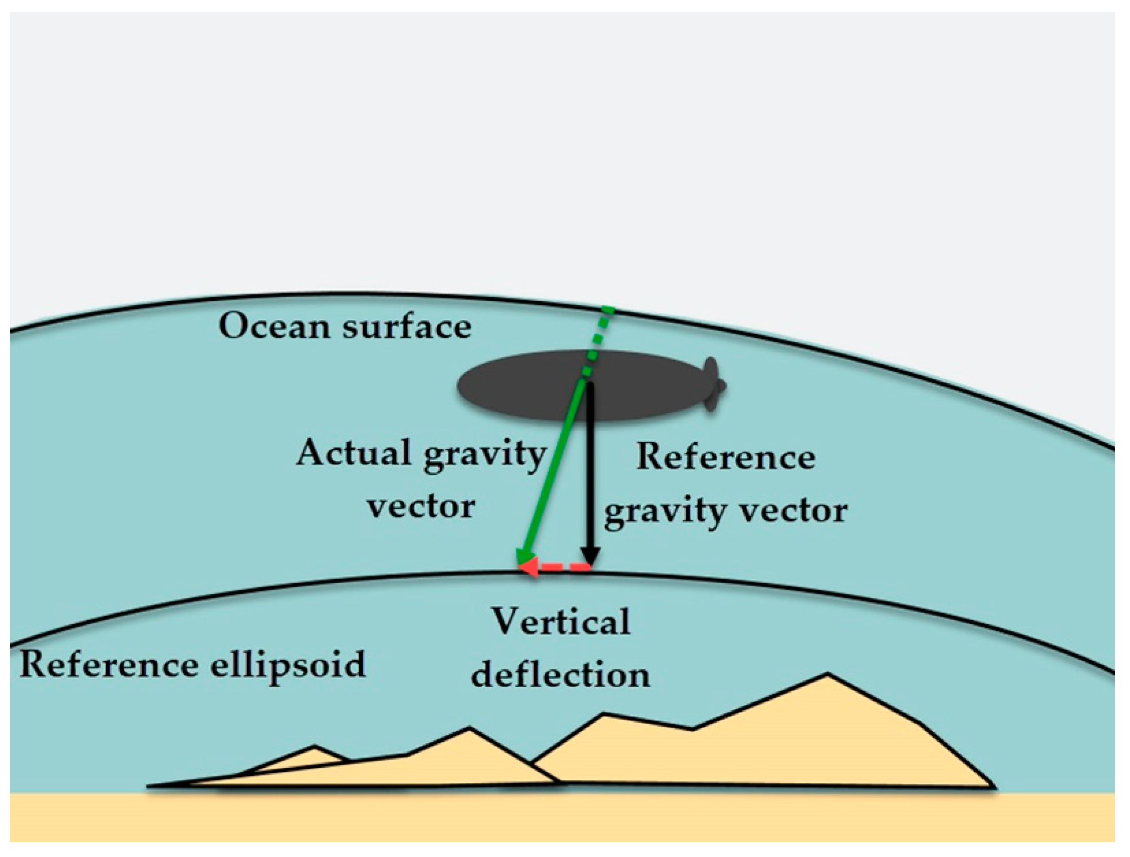
2.3.1. Gravity Navigation

As mentioned in Section 2.1, the earth’s gravitational field is far from being uniform and, for an INS, the effects of a change in the local gravitational field are indistinguishable from accelerations of the vehicle. One alternative is complementing the INS with gravity navigation. At the same time that an INS estimates the position of the vehicle, a gravity sensor—gravimeter or gradiometer—measures the gravity and gravity gradient where the AUV is located. A gravimeter measures gravity anomaly or the deviation in the magnitude of the gravity vector relative to a nominal earth model. A gradiometer is a pair of accelerometers with parallel input axes on a fixed baseline that measures gravity gradients or the rate of change of gravity with respect to linear displacement [29]. The difference in the accelerometer’s output excludes the linear vehicle acceleration but contains the gradient of gravitation across the baseline. Based on the position and the measurements from the sensor, the database searches for the best fit of gravity and gravity gradient, and then the optimal matching position will be used to correct the position error of the INS. Han et al. [58] proposed a matching algorithm for gravity aided navigation, combining an ICCP algorithm with a Point Mass Filter (PMF) algorithm. The algorithm involved a two-step matching process. First, the PMF based on vehicle position variable can obtain in real-time an instructional position given in a large initial position error. Then, the ICCP algorithm can be employed for further matching. In order to verify the validation of the proposed matching algorithm, a numerical simulation was performed with a 12 h sailing period, where the speed of the underwater vehicle was set to 10 nmi/h. Simulation tests indicated that compared with the conventional ICCP algorithm, the proposed algorithm can achieve better results in terms of latitude and longitude positioning errors, which were reduced up to 56% and up to 65% when compared with the INS standalone.

2.3.2. Geomagnetic Navigation

Geomagnetic Navigation relies on magnetic sensors and its essence is the Fitting of Two Point Sets (FTPS) process, where a marine geomagnetic map is used for matching [26]. Geomagnetic filed has many features which can be applied for matching [59], such as the intensity of the total field F, the horizontal component H, the north component X, the east component Y, the vertical component Z, the declination D, the inclination I, the geomagnetic gradient, and so on. These features are shown in Figure 9.

Zhao et al. [60] studied two matching algorithms, TERCOM and ICCP, used in the geomagnetic matching navigation. An experiment was designed to test the accuracy of the underwater navigation system, using a Differential GPS (DGPS) receiver for providing the exact position of the vehicle. In the results, matching positioning errors in the x direction or in the y direction were less than 100 m. Authors conclude that both TERCOM and ICCP can achieve credible geomagnetic navigation, with the difference that ICCP can provide a real-time positioning solution and TERCOM cannot. Ren et al. [7] presented a new algorithm to solve FTPS in geomagnetic localization. The algorithm was an improved version of the ICCP algorithm, based on the algorithm proposed by Menq et al. [61]. Simulation results showed that the ICCP-Menq-algorithm had a better performance than original ICCP algorithm in terms of dealing with geomagnetic-matching localization. Wang et al. [62] presented a new method which was based on the integration of TERCOM, K-means clustering algorithm and an INS. An experiment was implemented for evaluating the accuracy and the stability of the method proposed. INS and DGPS were set on the surveying vessel. In order to verify the accuracy of this new method, the positioning result from D-GPS is used for comparing with the result of the matching navigation. After completing the experiment, the error of the new method was under 50 m, meanwhile the traditional method showed an error up to 7 times higher.

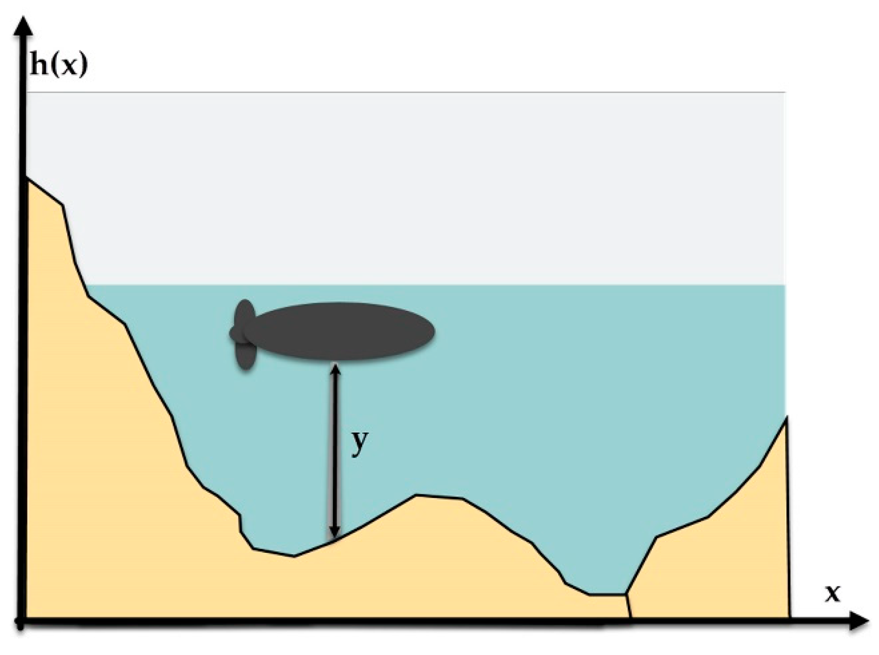
2.3.3. Bathymetric Navigation

One simple use of bathymetric maps for AUV navigation is the use of isobaths. An isobath is an imaginary curve that connects all points having the same depth below the surface. A controller [63] can be designed for an AUV to follow an isobath whit only low-level localization equipment—such as echo sounder—and ensures that it never leaves a pre-defined area. Terrain-Referenced Navigation (TRN), Terrain-Aided Navigation (TAN), and Terrain-Based Navigation (TBN) are all similar approaches for GN [64]. These systems estimate the errors in both a main navigation system—such as an INS—and the terrain database to provide a highly accurate position estimate relative to the digital terrain database. TBN operates by correlating the actual terrain profile overflow with the terrain information stored in the terrain database. A basic measurement equation [55] for TBN is given by:

$$\mathrm{y}=\mathrm{h}\left(\mathrm{x}\right)+\mathrm{e},$$

(8)

where h(·) is the terrain elevation function, x is the vehicle location, y is the measured terrain height, and e is the measurement noise. An example of terrain correlation in one dimension for a single altimeter measurement is represented in Figure 10.

Zhao et al. [65] worked on a TAN algorithm that combined TERCOM and PF. Experiments were performed to compare the proposed algorithm with the BITAN II algorithm. Results showed that the North and East position error remained below 100 m for the new algorithm, and the mean error was less than half of the mean error for the BITAN-II algorithm. Based on those results, authors concluded than their system was more reliable, possessed a higher positioning precision and a better stability than the one used for comparison.

Salavasidis et al. [66] proposed a low-complexity PF-based TAN algorithm for a long-range, long-endurance deep-rated AUV. The potential of the algorithm was investigated by testing its performance using field data from three deep (up to 3700 m) and long-range (up to 195 km in 77 h) missions performed in the Southern Ocean. Authors compared TAN results to position estimates through DR and USBL measurements. Results showed that TAN holds a potential to extend underwater missions to hundreds of kilometers without the need for surfacing to re-initialize the estimation process. For some of the missions analyzed, the RMSE of the TAN algorithm was up to 7 times lower when compared with the DR measurements and the absolute water-depth difference was reduced up to 66% when compared with USBL measurements. Meduna et al. [67] proposed a TRN system for vehicles with low-grade navigation sensors, with the aim of improving navigation capabilities of simple DR systems. The algorithm uses an 8-dimensional particle filter for estimating critical motion sensor errors observed in the vehicle. Field trials were performed on an AUV with DR navigational accuracy of 5–25% of Distance Traveled (DT). The ability of TRN to provide 5–10 m navigational precision and an online return-to-site capability was demonstrated.

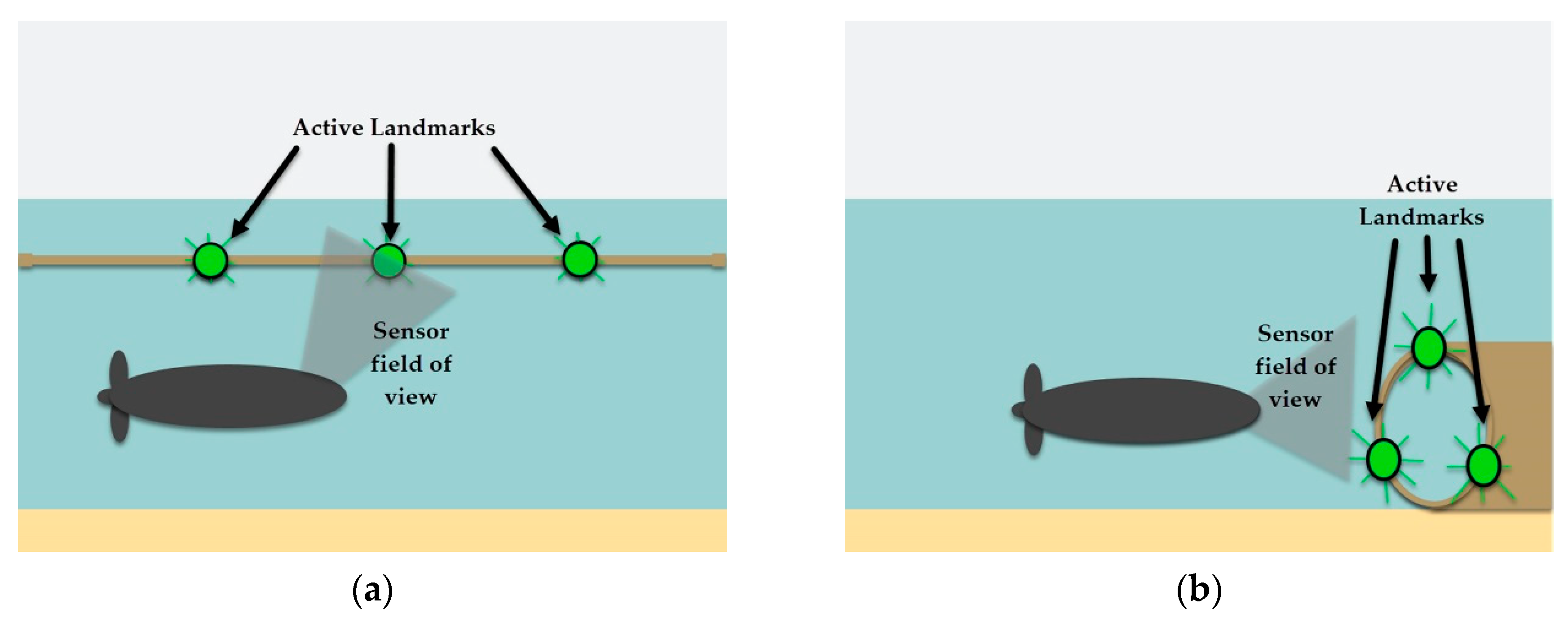
2.4. Optical Navigation

Optical technologies are a relevant option to provide information about the environment. These systems can be implemented either with a camera or with an array of optical sensors. Despite the poor transmission of light through water, which results in a limited range for imaging systems [68], different algorithms and techniques are being studied for this purpose. In Figure 11, two examples of optical systems are shown; where the AUV must detect and follow active landmarks within a structure (a) or identify a pattern made with active marks to navigate through it (b).

An optical detector array sensor system was presented for AUV navigation by Eren et al. [69]. The performance of the developed optical detector array was evaluated for its capability to estimate the position, orientation and forward velocity of AUVs regarding a light source fixed underwater. The results of computational simulations showed that a hemispherical frame design with a 5 × 5 photo-detector array was sufficient to generate the desired position and orientation feedback to the AUV with a detection accuracy of 0.2 m in translation (surge, sway, and heave) and 10° in orientation (pitch and yaw) based on a spectral angle mapper algorithm. Some of these optical or artificial vision systems have been applied to AUVs for different purposes such as docking and recovery. Zhong et al. [70] developed an artificial vision system capable of detecting a set of lamps located around the desired docking location for an AUV. The AUV uses a binocular localization method to locate the docking platform and navigates to reach it. Navigation lamps were mounted at the entrance of the docking station as active beacons. Three common underwater green lamps were symmetrically positioned on the docking model around the center of the three lamps. An experiment using a ship model has been conducted in a laboratory to evaluate the feasibility of the algorithm. The test results demonstrated that the average localization error is approximately 5 cm and the average relative location error is approximately 2% in the range of 3.6 m. A similar approach was proposed by Liu et al. [71]. A vision-based framework for automatically recovering an AUV by another AUV in shallow water was presented in this work. The proposed framework contains a detection phase for the robust detection of underwater landmarks mounted on the docking station in shallow water, and a pose-estimation phase for estimating the pose between AUVs and underwater landmarks. At ground experiments, they observed that the mean position and orientation errors were 1.823° and 6.306 mm, respectively, in the absence of noise, and 2.770° and 9.818 mm, respectively, in the presence of strong noise. Field experiments were performed to recover a sub-AUV by a mother vessel in a lake using the proposed framework and experiments showed that the algorithm outperformed the state-of-the-art method in terms of localization error.

Although these systems showed a response with high accuracy, pre-installed infrastructure is needed to implement them. An alternative approach is the use of a camera or set of cameras to identify features in the environment or targets for the AUV mission. Monroy et al. [72] developed a micro AUV with an artificial vision system that allows it to follow an object by its color. A Hue Saturation Value (HSV) filter was implemented on the artificial vision system and a non-linear proportional-derivative controller on the vehicle to stabilize the heave and surge movements. A search and recovery problem is addressed by an intervention AUV by Prats et al. [73]. The problem consisted of finding and recovering a flight data recorder. The mission is compounded by two stages: survey and intervention. As the system was tested on a water tank, the survey stage consisted of a pre-defined trajectory of the AUV. This trajectory guarantees that images taken by the AUV cameras cover the complete bottom of the tank. Once the survey is complete, the flight data recorder is identified on the images by applying an HSV histogram and then located; so, the intervention stage can take place. Even though these techniques are quite popular on land and air robots, working this way has several restrictions at underwater. It is required to know before the mission what the robot is looking for; the robot must be pointed to an object of potential interest and HSV boundaries must be manually selected until it is well detected; it also has the inconvenience that colors are not the same underwater as above water, because they are strongly affected by illumination.

2.5. Simultaneous Location And Mapping (SLAM)

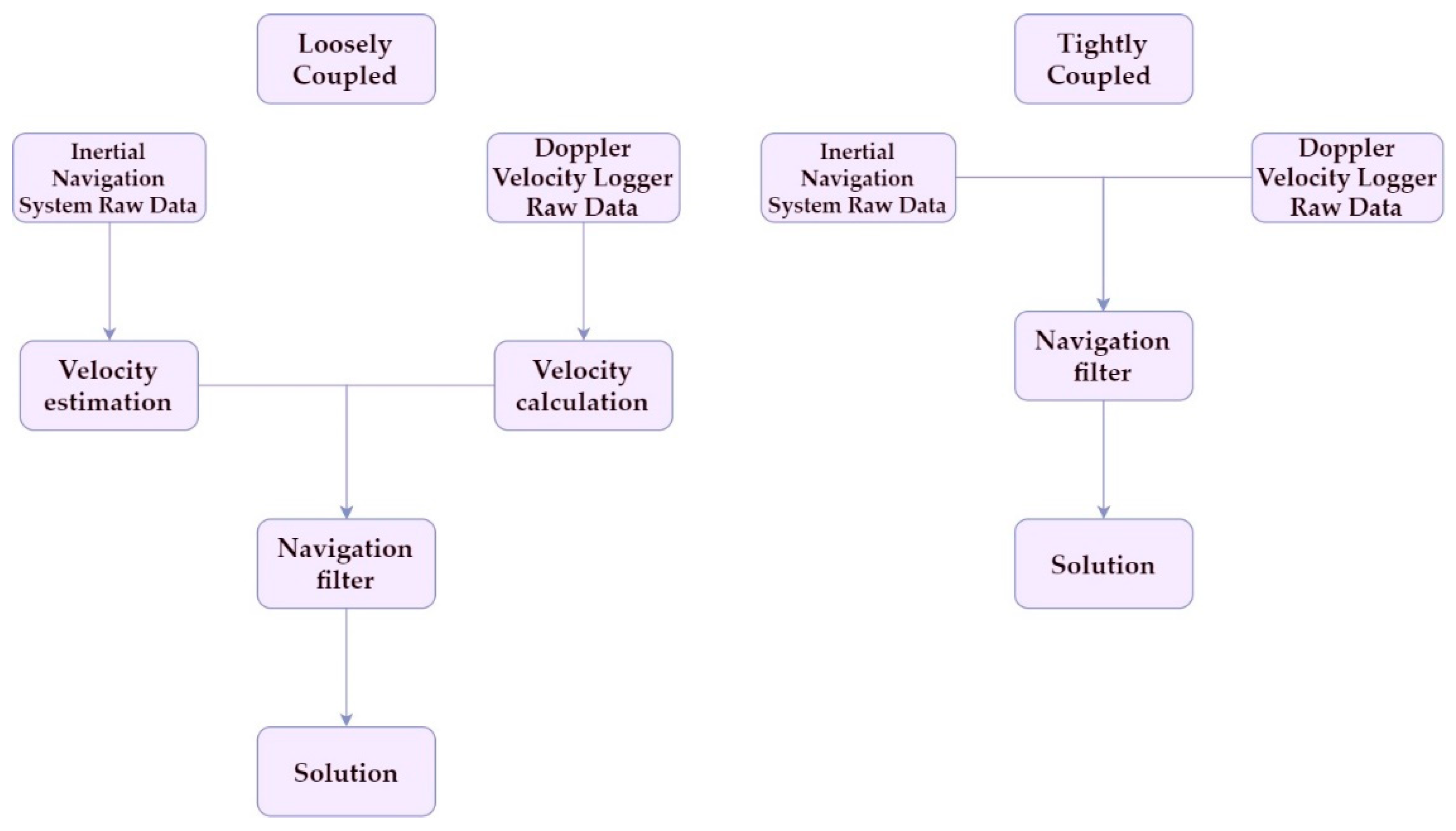
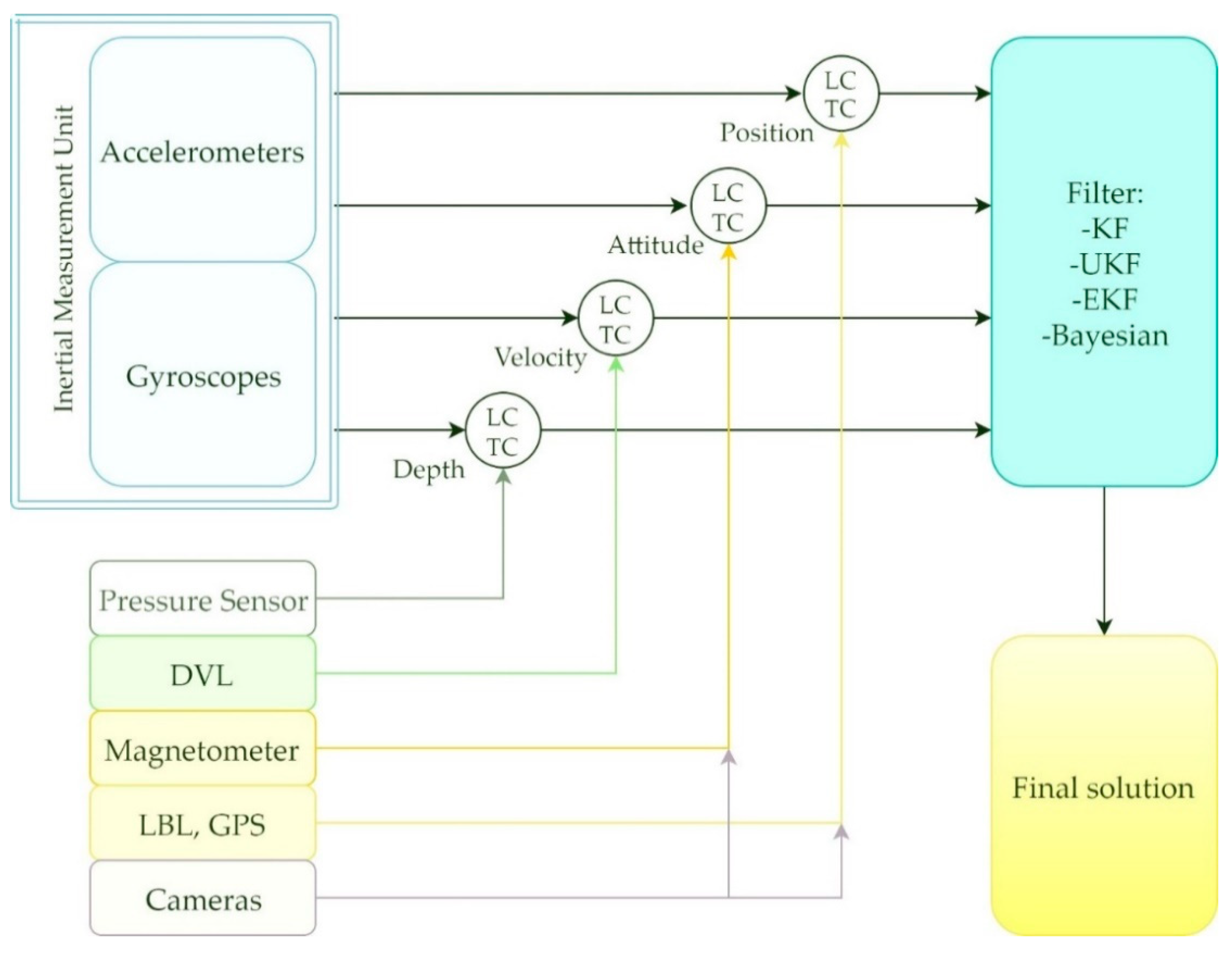
Simultaneous Location and Mapping (SLAM) is a technique that consists of a mobile robot, such as an AUV, being placed at an unknown location in an unknown environment and make it able to build a consistent map of the environment and determinate its location within this map [74]. In Figure 12, a SLAM solution is represented where an AUV is equipped with a sensor to explore the environment to create a digital reconstruction of it. Color codes can be used to represent information such as distance between the vehicle and obstacles.

There are different SLAM representation methods used to reconstruct the environment. Each one has its own shortcomings and advantages, choosing the best one depends on the application desired which can be inspection, navigation, interaction, etc. The principal representation methods are listed in

Table 3. SLAM representation methods.

Method	Type	Description	Applications
landmark-based maps	2D/3D	Models the environment as a set of landmarks extracted from features as points, lines, corners, etc.	Localization and mapping [75].
Occupancy grid maps	2D	Discretizes the environment in cells and assigns a probability of occupancy of each cell.	Exploring and mapping [76].
Raw Dense Representations	3D	Describes the 3-D geometry by a large unstructured set of points or polygons.	Obstacle avoidance and visualization [77].
Boundary and Spatial-Partitioning Dense Representations	3D	Generates representations of boundaries, surfaces, and volumes.	Obstacle avoidance and manipulation [78].

.

Underwater SLAM can be categorized in acoustic-based and vision-based [38]. The perception of optical devices is constrained by poor visibility and noise produced by sunlight in shallow waters. Moreover, they can provide high frequencies and high resolution for a lower cost than an acoustic system. On the other hand, a high-definition FLS can provide a promising alternative for working under challenging conditions.

In [79], Hernández et al. presented a framework to give an AUV the capability to explore unknown environments and create a 3D map simultaneously with an acoustic system. The framework comprises two main functional pipelines. The first, provides the AUV with the capacity of creating an acoustic map online, while planning collision-free paths. The second pipeline builds a photo-realistic 3D model using the gathered image data. This framework was tested in several sea missions where results validated its capabilities. Palomer et al. [80] used a multi-beam echo-sounder to produce high consistency underwater maps. Since there is not a general method to evaluate consistency of a map, authors computed the consistency-based error [81] and proposed a 3D statistic method named #Cells. The statistic method consisted in counting the number of cells that each bathymetric map occupies within the same 3D grid. If a map occupies less cells, it is probably because their point clouds are more densely packed due to a better registration. The algorithm was tested using two real world datasets. Three surfaces were created for different navigation methods: DR, USBL and the proposed algorithm. Regarding the number of occupied cells, the proposed method occupied 5.76% less cells than a DR model, and 7.24% less than the USBL model.

Gomez-Ojeda et al. [82] implemented a visual-based SLAM algorithm. Authors compared a stereo Point and Line SLAM (PL-SLAM) with an Orientated FAST and Rotated BRIEF (ORB) SLAM, a point-only system and a line-only system. Results showed superior performance of the PL-SLAM approach relatively to ORB-SLAM, in terms of both accuracy and robustness in most of the dataset sequences. The mean translational error was minor for PL-SLAM in 55% of the sequences and the mean rotational error in the 73% of the cases. Nevertheless, that work was not tested for underwater applications. After that, Wang et al. [83] proposed a method to improve the accuracy of vision-based localization systems in feature-poor underwater environments using PL-SLAM algorithm for localization. Three experiments were performed, including walking along the wall of a pool, walking along a linear route, and walking along an irregular route. The experimental results showed that the algorithm was highly robust in underwater low-texture environments due to the inclusion of line segments. At the same time, the algorithm achieved a high accuracy of location effectively. The attitude error—computed as shown in Equation (8)—was 0.1489 m, which represented the 2.98% DT.

$$\mathrm{Attitude}\mathrm{error}=\sqrt{{\left(\mathrm{error}\_\mathrm{x}\right)}^2+{\left(\mathrm{error}\_\mathrm{y}\right)}^2+{\left(\mathrm{error}\_\mathrm{z}\right)}^2}$$

(9)

Authors conclude that it can be implemented in the navigation and path planning of AUVs in the future. With the aim to explore the capabilities of visual-based SLAM in real and challenging environments, Ferrera et al. [84] proposed what they considered as the first underwater dataset dedicated to the study of underwater localization methods from low-cost sensors. The dataset has been recorded in a harbor and provides several sequences with synchronized measurements from a monocular camera, a Micro-Electro-Mechanical System-Inertial Measurement Unit (MEMS-IMU) and a Pressure Sensor (PS). Among the sensors used in the dataset acquisition were a 20 frames per second (fps), 600 × 512 px monochromatic camera, and a 200 Hz IMU. As a benchmark, authors ran experiments using state-of-the-art monocular SLAM algorithms, and then compared ORB-SLAM, Semi-direct Visual Odometry (SVO) and Direct Sparse Odometry (DSO). Results showed an absolute translation error between 24–52 cm, 24–67 cm, and 2–56 cm for each of the methods applied, which highlighted the potential of vision-based localization methods for underwater environments. With the same idea, Joshi et al. [85] formed their own datasets from an underwater sensor suite—equipped with a 100 Hz IMU and a 15 fps, 1600 × 1200 px stereo camera—operated by a diver, an underwater sensor suite mounted on a diver propulsion vehicle, and an AUV. Experiments were conducted for each dataset considering the following combinations: monocular; monocular with IMU; stereo; and stereo with IMU, based on the modes supported by each Visual Odometry (VO) or Visual Inertial Odometry (VIO) algorithm. Results showed that DSO and SVO, despite quite often fail to track the complete trajectory, had the best reconstructions for the tracked parts and, as expected, stereo performed better than monocular. The results confirmed that incorporating IMU measurements drastically lead to higher performance, in comparison to the pure VO packages.

2.6. Sensor Fusion

As established in Section 2.1, the main inconvenient of an INS is that the position and orientation accuracy drifts over time, so, to keep it under the limits expected for safe AUV navigation, the system must correct its error by comparing its position estimation with a fixed location measured from additional sensors—such as a GPS—periodically. To overcome this, the INS can be fused with other sensors. There are two main schemes for sensor fusion: loosely coupled (LC) and tightly coupled (TC). The basic difference is the data shared by the sensors. In an LC scheme, a solution for the position or orientation of the AUV is obtained for each sensor individually and then blended using a filter—such as a Kalman Filter (KF)—to obtain a more accurate and reliable solution. In a TC scheme, raw measurements of the sensors are processed directly on the filter to overcome problems as poor signal quality or limited coverage thanks to the filter’s capabilities to predict the pose of the vehicle. In this case, a more robust filter is needed so variants of the KF are commonly used [86], such as an EKF or Unscented Kalman Filter (UKF). Filter selection is essential to get a better solution for the vehicle’s pose and, besides the sensor fusion approach adopted, accuracy, numerical efficiency, and computational complexity must be considered. LC and TC schemes are represented in Figure 13 with velocity estimation from an INS and a Doppler Velocity Logger (DVL) as example.

Most of the sensor fusion systems for AUV navigation are those of an INS aided by a DVL; typically, the fusion is under an LC scheme [87,88,89] with a linear filter. However, in cases where the DVL measurements are limited, an LC algorithm leaves the INS to work alone. This produces an accumulative error which gets bigger with time. Considering this, Liu et al. [90] explored a TC scheme as an alternative. This approach includes depth updates given by a depth sensor among to raw measurements from the DVL to help the INS and avoid the drift caused by limited measurements on the LC approach. Different trajectories were simulated for an AUV including a straight line at a for 1,800 s with a constant velocity. For simulations, the update frequencies of the INS, DVL, and PS were 200 Hz, 1 Hz, and 1 Hz, respectively. For x, y, and z axes, a gyro drift of 0.01°/h and a 100 μg accelerometer bias were introduced as INS errors; 0.002 m/s as a constant DVL error, and 0.05 m as a constant PS error. The results showed a cumulative error of 1000 m at the end of the trajectory for the LC approach and only 10 m in the TC case. Same disadvantages of the LC fusion of an INS/DVL system was addressed by Tal et al. [91]. In their work, they designed a navigation system based on a 150 Hz INS aided with a 1 Hz DVL, a 0.5 Hz magnetometer, and a 0.25 Hz PS under an Extended Loosely Coupled (ELC) approach within an EKF. They focused their work in exploring cases where only partial measurements of the DVL were available and used external information to complete the velocity calculation of the vehicle. To test their system, different trajectories of a vehicle were simulated. Results showed a better performance by the ELC scheme, with improvements up to 38% on Root-Mean-Square Errors when compared with the standalone INS and up to 12% compared with a TC scheme.

Another approach is the fusion of INS with acoustic systems. In [92,93], Zhang et al. investigated the use of an AUV positioning method based on a SINS and an LBL under a TC algorithm. Authors were looking to solve position error accumulation of AUVs. They compared the TC and LC approaches by simulating an AUV trajectory under different conditions, such as changing the number of hydrophones available. Test results demonstrated that the system proposed in this work is more reliable than LC approach since the error on the trajectory—particularly when approaching or leaving the hydrophones array—was up to 50% lower.

Artificial vision is also being fused with INS to improve its performance. Manzanilla et al. [94] addressed autonomous navigation for AUVs. They used artificial vision fused with an IMU on a LC algorithm. Parallel Tracking and Mapping (PTAM) was implemented to localize the vehicle respect to a visual map, using a single camera—15 fps, 640 × 480 px. Then, an EKF was used to fuse the visual information with data from an IMU, to recover the scale of the map and improve the pose estimation. In this work, fully autonomous trajectory tracking was successfully achieved and compared using standalone PTAM and the sensor fusion approach. Results showed that the trajectory followed by the vehicle using sensor fusion has errors not bigger than 20 cm whilst the standalone PTAM drift up to 60 cm.

The EKF is the most widely used nonlinear filtering approach in TC schemes. EKF is based on a simple linear approximation to the nonlinear equations. However, there are too many unknown disturbance factors at underwater, and they cannot be established in suitable mathematical models in the kinematic equation. Other alternatives to a traditional EKF have been explored. Li et al. [95] proposed a multi-model EKF integrated navigation algorithm. It was designed to solve the harsh underwater environment problems. This algorithm, based on the probabilistic data association theory, was compared with standard EKF in a lake trial using an AUV equipped with an IMU, an AHRS, and an LBL system with four acoustic beacons. Results showed a better performance by the multi-model EKF since the error between true positions and estimations were less than 12 m. The algorithm showed to be able to overcome disturbances that produced peaks of over 400 m on traditional EKF estimations. Chen et al. [96] worked on another alternative to an EKF for TC SINS/LBL navigation systems. Instead of applying an EKF they used a near-real-time (NRT) Bayesian framework. They compared NRT framework with EKF approaches with an accurate and a poor initialization. Results showed a better performance by the NRT solution with an 80% reduction of the measurement residuals with a poor accurate yaw error initialization.

The main alternatives for sensor fusion based on an INS are summarized in Figure 14.

2.7. Localization and Navigation Overview

General conclusions in terms of sensors performance for non-traditional AUV navigation and localization technologies are shown in

Table 4. Technologies for AUV localization and navigation.

Navigation Technology	Approaches	Information Available	Accuracy	Range	Results
Acoustic	SONAR	Distance from obstacles.	Depending on distance from obstacles, from 5–10 cm to more than a meter (10–120 cm).	From 5 m up to hundreds of meters from obstacles.	Experimental in real conditions.
	Acoustic range (LBL, SBL, USBL).	Position	Depending on distance from hydrophone array and the frequency, from some centimeters up to tens of meters.	Up to tens of meters from the array.	Experimental in real conditions.
Geophysical	Gravity, geomagnetic, TAN, TRN, TBN	Position	Meters. Depending on the map resolution and filter applied.	Kilometers from initial position.	Simulation, Experimental under controlled conditions.
Optical	Light sensors.	Position and orientation relative to a target.	Up to 20 cm for position and 10° for orientation.	1–20 m from markers.	Simulation, Experimental under controlled conditions.
	Cameras		Up to 1 cm for position and 3° for orientation.	1–20 m from markers.	Experimental in real conditions.
SLAM	Acoustic	Position and orientation relative to the mapped environment.	From some centimeters up to more than a meter.	Up to tens of meters from targets.	Experimental in real conditions.
	Cameras			1–10 m from targets.	Simulations, Experimental under controlled conditions.
Sensor fusion	ELC, LC, TC.	Position, orientation and velocity.	Depending on the approach and filter applied, accumulative error can be reduced up to some meters (5–20)	Kilometers from initial position.	Simulations, Experimental.

.

After the literature review, it can be considered that acoustic-based technologies still a reliable alternative for AUV localization and navigation; although they require more infrastructure than others. Future work must consider the possibility to include them in teams of collaborative AUVs. To achieve that, acoustic systems must overcome low updated rates and limited accuracy (at long ranges) in order to avoid collisions in AUV formations, especially when they are navigating in a few meters of each other. On the other hand, visual-based localization technologies—including SLAM—have gained attention in recent years. These technologies can estimate both, position and orientation, contrary to acoustic methods. They also reach a higher accuracy which is critical for the collaborative navigation of AUVs. Thus, it is an interesting and reliable option for some particular tasks under specific environments. Nevertheless, most of them are on an early level of readiness since they have been tested only in very controlled environments. It seems difficult for visual-based systems to overcome the challenging conditions of underwater. Moreover, it is hard for researches to find the proper conditions to test their visual-based and visual-SLAM algorithms in real underwater conditions. To deal with that, some datasets are being collected such as the AQUALOC dataset [97], which is dedicated to the development of SLAM methods for underwater vehicles navigating close to the seabed. The Autonomous Field Robotics Laboratory (AFRB) [98] has some datasets available for the same purpose.

3. Collaborative AUVs

Once the navigation and localization problem for the AUVs is solved, a scheme for collaborative work between a group of robots can be proposed. Collaborative work refers to an interaction of two or more AUVs to perform a common task which can be collaborative navigation, exploration, target search, and object manipulation. Using a team of AUVs navigating on a certain formation has the potential to significantly expand the applications for underwater missions; such as those that require proximity to the seafloor or to cover a wide area for search, recovery, or reconstruction. At first, researchers focused their work on how multiple vehicles could obtain data simultaneously from the same area of interest. Nowadays, their focus has moved to the trajectory design and operation strategies for those multi-vehicle systems [99].

3.1. Communication

The rapid attenuation of higher frequency signals and the unstructured nature of the undersea environment make difficult to establish a radio communication system for AUVs. For those reasons, wireless transmission of signals underwater—especially for distances longer than 100 m—relies almost only on acoustic waves [14,100]. Underwater acoustic communication using acoustic modems consists of transforming a digital message into sound that can be transmitted under water. The performance of these systems changes dramatically depending on the application and the range of operation [101]. The main factors to choose an underwater acoustic modem are:

• Application: Consider the type and length of message (Command and control messages, voice messages, image streaming, etc.) frequency of operation and operating depth.
• Cost: Depending on the complexity and performance, from some hundreds up to $50,000 (USD).
• Size: Usually cylindrical, with lengths from 10 cm to 50 cm.
• Bandwidth: Acoustic modems can perform underwater communication at up to some kb/s. Length of the message and time limitations must be considered
• Range: Range of operation for the vehicle’s communication has impact on the cost of the system. Acoustic modems are suitable from short distances up to tens of km. Considerer than a longer range will increase the latency and power consumption of the system.
• Power consumption: Depending on the range and modulation, the power consumption is in the range of 0.1 W to 1 W in receiving mode and 10 W to 100 W in transmission mode.

Table 5. Commercial acoustic modems.

Name	Max Bit Rate (bps)	Range (m)	Frequency Band (kHz)
Teledyne Benthos ATM-925 [102]	360	2000–6000	9–27
WHOI Micromodem [103]	5400	3000	16–21
Linkquest UWM 1000 [104]	7000	350	27–45
Evologics S2C R 48/78 [105]	31,200	1000	48–78
Sercel MATS 3G 34 kHz [106]	24,600	5000	30–39
L3 Oceania GPM-300 [107]	1200	45,000	Not specified
Tritech Micron Data Modem [108]	40	500	20–28
Bluerobotics Water Linked M64 Acoustic Modem [109]	64	200	100–200

contains a few options of acoustic modems commercially available.

The working principles of underwater acoustic communication can be described as follows [110]: First, information is converted into an electrical signal by an electrical transmitter. Second, after digital processing by an encoder, the transducer converts the electrical signal into an acoustic signal. Third, the acoustic signal propagates through the medium of water and propagates the information to the receiving transducer. In this case, the acoustic signal is converted into an electrical signal. Finally, after the digital signal is deciphered by the decoder, the information is converted to an audio, text or picture by the electrical receiver.

Acoustic communications face many challenges, such as, small bandwidth, low data rate, high latency, and ambient noise [111]. These shortcomings might provoke that a cycle of communication in a collaborative mission take several seconds, or even more than a minute. Considering these, Yang et al. [112] analyzed formation control protocols for multiple underwater vehicles in the presence of communication flaws and uncertainties. The error Port-Hamiltonian model about the desired trajectory was introduced and then, with the existence of relative information constraints or uncertainties, the formation control law was achieved by solving specific limitations of the linear matrix inequality problem. Abad et al. [113] introduced a communication scheme between the AUVs and a unique representation of the overall vehicle state that limits message size. To limit data sent, every reported position and path plan is encoded using a grid encoding scheme. Authors implemented a decentralized model predictive control algorithm—centralized schemes are typical for swarms of AUVs—to control teams of AUVs that optimizes vehicle control inputs to account for the limitations of operating in an underwater environment. They simulate their proposal and showed the effectiveness of their approach in a Mine/Countermine mission. Other way to deal with acoustic communication issues was presented by Hallin et al. [114]. They proposed that enabling the AUVs to anticipate acoustic messages would improve their ability to successfully complete missions. They outlined an approach to AUV message anticipation in AUVish-BBM (BBM suffix includes the initials of the researchers directly involved in dialect development: Beidler, Bean and Merrill [115]), an acoustic communications language for AUVs [116], based on a University of Idaho-developed paradigm called Language-Centered Intelligence (LCI). They demonstrated a new application of LCI in the field of cooperative AUV operations and argued that message anticipation can be effectively deployed to correct message errors. The structure, content, and context of individual messages of AUVish-BBM, together with its associated communication protocol, supply a systematic framework that can be utilized to anticipate messages expressed by AUVs performing collaborative missions.

The absence of an underwater communication standard has been a problem for collaborative teams of AUVs. In 2014, Potter et al. presented the JANUS underwater communication standard [117], a basic and robust tool for collaborative underwater communications designed and tested by the NATO Centre for Maritime Research and Experimentation. This opened the possibilities for simple integration of different robots using this standard [118,119,120,121] for collaborative tasks as underwater surveillance.

To improve the performance of underwater communication, optical technologies have been tested either stand-alone [122,123] or as a complement for an acoustic system [100]. Laser submarine communication has some advantages such as a high bit rate, higher security and broad bandwidth. Blue-green light (whose wavelength is 470–580 nm) penetrates water better and its energy attenuation is less than any other wavelength light [124]. Thus, researchers have explored optical underwater communication systems based in blue-green light, to allow an underwater vehicle to receive a message from an aerial/spatial system at any depth despite its actual speed, course and distance from the transmitter. Wiener et al. [122] were seeking for a system to deliver a message from a satellite to a submarine, avoiding the need for the submarine to navigate close to the surface for retrieving the message as happened with the radio-frequency systems used at the time. Authors stated that blue light has the potential to accomplish the result expected in the future. However, their research was only a brief representation of what could be expected when working in such a difficult environment. Puschell et al. [123] performed the first demonstration of a two-way laser communication between a submarine vehicle and an aircraft; and concluded that a blue-green laser communication system could, someday, reach operational requirements. Sangeetha et al. [125] made experiments to study the optical communication between an underwater body and a space platform using a red laser with a 635 nm wavelength. Results showed that the performance of the red-light system was lower than the expected for a blue-light system in terms of the attenuation coefficient observed. Corsini et al. [126] worked on an optical wireless communication system where both, transmitter and receiver, where at underwater. The optical signal with a 470 nm wavelength was obtained modulating two LED arrays and received by an avalanche photodiode module. Error free transmission was achieved in the three configurations under test (6.25 Mbit/s, 12.5 Mbit/s, and 58 Mbit/s) through 2.5 m clean water.

Despite some authors as Wiener and Puschell have claimed that laser communication systems for underwater vehicles could be a possibility, recent studies showed that technology still limited. Laser-based systems cannot reach a target with a more than a few tens of meters depth under ideal conditions [127]. Thus, Farr et al. [100] developed an optical communication system that complements and integrates an acoustic system. The result was an underwater communication system capable to offer high data rates and low latency when within optical range; combined with long range and robustness of acoustics when outside of optical range. Authors have demonstrated robust multi-point, low power omnidirectional optical communications over ranges of 100 m at data rates up to 10 Mb/s using blue-green emitters.

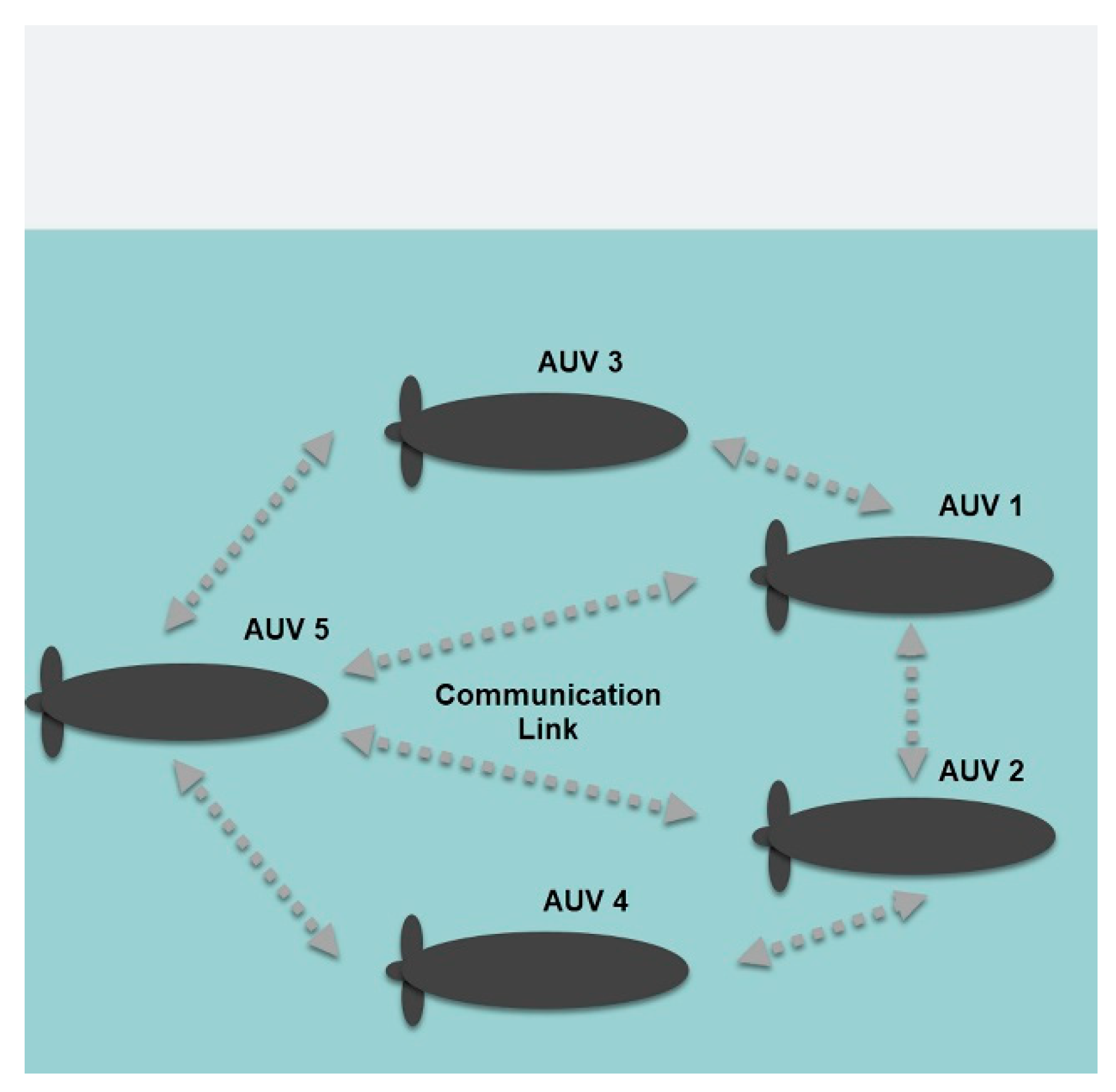
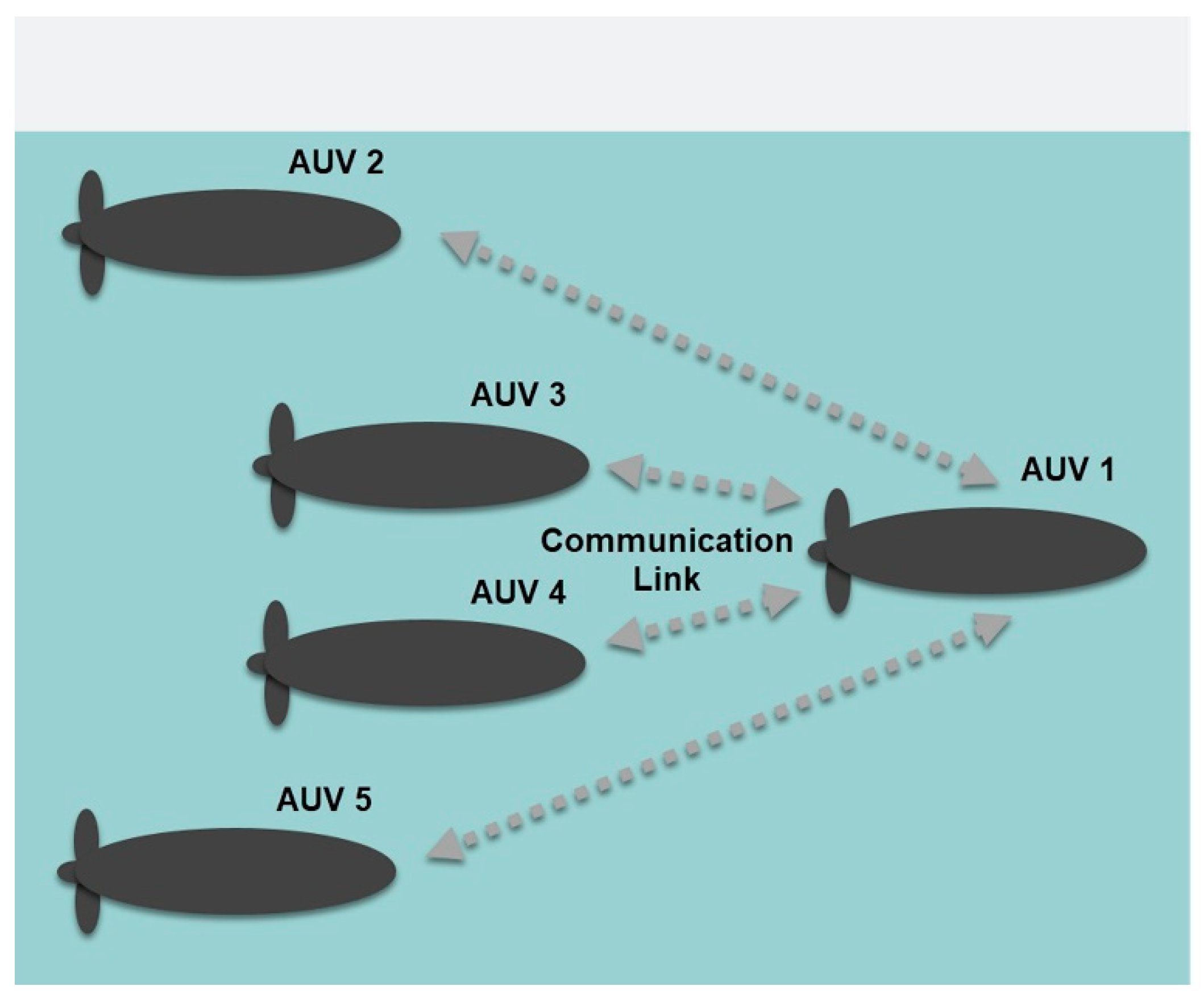
3.2. Collaborative Navigation

Groups of AUVs can work together under different navigation schemes, which are generally parallel or leader-follower [110]. On a parallel formation (shown in Figure 15), all AUVs are equipped with the same systems and sensors, to locate and navigate themselves precisely and to communicate with its neighbor AUVs.

In a leader-follower scheme (shown in Figure 16), leader AUV is equipped with high-precision instruments meanwhile follower AUVs are equipped with low-precision equipment [128]. Communication is only required between the vehicle leader and its followers, there is no need for the followers to communicate with each other.

The lower cost and the reduced communications needs make the leader-follower scheme the main navigation control method of AUVs. Its basic principles and algorithms are relatively mature [110]. However, unstable communications and communication delays are still challenging problems and need to be addressed. Since there are problems with signals when multiple systems emit at the same time, co-localization of AUVs is mostly based on time synchronization. However, time synchronization methods have some shortcomings such as the need for AUVs to go to surface to receive the synchronization signal. As an alternative, Zhang et al. [129] studied multi-AUVs collaborative navigation and positioning without time synchronization. Authors established a collaborative navigation positioning model for multi-AUVs and designed an EKF for collaborative navigation. This design only needs the time delay of the AUV itself and does not need to consider whether the AUV has synchronized with others. In simulated experiments, they compared the precision of their algorithm with a prediction model and results showed that, even when error increases over time, the precision of co-localization without time synchronization was higher. Yan et al. [130] addressed the problems of leader-follower AUV formation control with model uncertainties, current disturbances, and unstable communication. The effectiveness of the method is simulated by tracking a spiral helix curve path with one leader AUV and four follower AUVs. Considering model uncertainties and current disturbances, a second-order integral AUV model with a nonlinear function and current disturbances was established. The simulation results showed that leader-follower AUV formation controllers are feasible and effective. After an adjustment period, all follower AUVs can converge to the desired formation structure, and the formation can keep tracking the desired path.

Cui et al. [131] focused on the problem of tracking control for multi-AUV systems and proposed an adaptive fuzzy-finite time control method. In this algorithm, algebraic graph theory is combined with a leader-follower architecture for describing the communication of the system. Then, the error compensation mechanism is introduced. Finally, the application of finite time and fuzzy logic system improves the convergence rate and the robustness of multi-AUV system. The effectiveness of the proposed algorithm was illustrated by simulation. Choosing the architecture of 4 AUVs including 1 leader and 3 followers. In order to avoid the unknown internal and external interferences, the algebraic graph theory and a fuzzy logic system technique are integrated into the distributed controllers. The simulation results demonstrate the effectiveness of the proposed algorithm and robustness of the multi-AUV system with a faster convergence speed compared with others algorithms.

When AUVs navigate in closed formations, the delay between the transmission and reception of the acoustic signals represents a high risk. Therefore, a solution with a response time significantly faster must be explored. Bosh J. et al. [11] developed an algorithm for AUVs navigating on a close formation, where light markers and artificial vision are used to allow the estimation of the pose of a target vehicle at short ranges with high accuracy and execution speed. In the experiments presented, the filtered pose estimates were updated at approximately 16 Hz, with a standard deviation lower than 0.2 m in the distance uncertainty between vehicles, at distances between 6 m and 12 m. As expected, the results showed that the system performs adequately for vehicle separations smaller than 10 m, while the tracking becomes intermittent for longer distances due to the challenging visibility conditions underwater.

Other alternatives for cooperative navigation of AUVs is the use of systems that allow the vehicles within a team to help each other with their localization. Teck et al. [132] proposed a TBN system for cooperative AUVs. The approach consists on an altimeter and acoustic modem equipped on each vehicle and a bathymetric terrain map. The localization is performed via decentralized particle filtering. The vehicles in the team are assumed to have their system time synchronized. A simple scheduling is adopted so that each vehicle in the team broadcasts its local state information sequentially using acoustic communication. This information includes the vehicle current position, the filter estimated covariance matrix, and the latest water depth measurement. When the acoustic signal is received by another vehicle the time-of-arrival can be calculated to determine the inter-vehicle distance. Results showed that localization performance improves as the number of the vehicles in the team increase, at least up to four, and when they are in range for a proper acoustic communication. The average positioning error was in the range of a few meters in those conditions. Tan et al. [133] developed a cooperative path planning for range-only localization. Authors explored the use of a single-beacon vehicle for range-only localization to support other AUVs. Specifically, they focused on cooperative path-planning algorithms for the beacon vehicle using dynamic programming formulations. These formulations take into account and minimize the positioning errors being accumulated by the supported AUV. Implementation of the cooperative path-planning algorithms was in a simulated environment. The simulations were conducted with different types of ranging aids, each transmitted from a single beacon. The ranging aids used were: single fixed beacon, circularly moving beacon, and cooperative beacon. Experimental results were also obtained by a field trial was conducted near Serangoon Island, Singapore. Average error was reduced up to 19.1 m over a traveled distance of 1.5 km. De Palma et al. [134] made a similar approach. The problem addressed by the authors consisted of designing a relative localization solution for a networked group of vehicles measuring mutual ranges. The aim of the project was to exploit inter-vehicle communications to enhance the range-based relative position estimation. Vehicles are considered capable to know their own position, orientation, and velocity regarding a common frame. Such vehicles share their own information through their communication channel and they can obtain measurements of their relative Euclidean distance with respect to several other agents. The connection topology of the agents was represented through a relative position measurement graph and a simulation, relative to a group of 4 agents, was performed with different connection topologies. During the simulation, z error remained in the range of ± 1 m after a time-lapse of 3000 s.

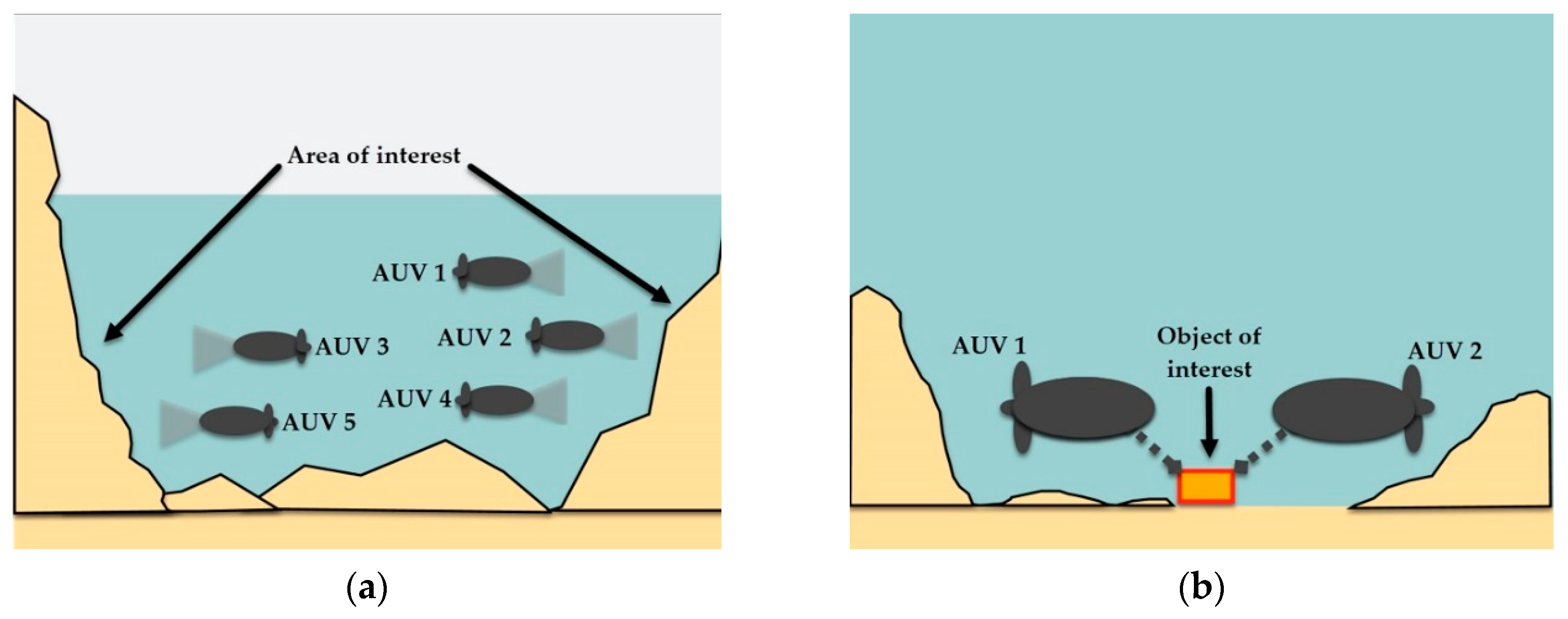
3.3. Collaborative Missions

Surveillance and intervention are typically the kinds of missions designed for teams of AUVs. Surveillance missions require the AUVs to detect, localize, follow, and classify targets, inspect or explore the ocean. Meanwhile, intervention missions require the AUVs to interact with objects within the environment. Examples of both missions are represented in Figure 17.

3.3.1. Search Missions

A good search mission needs to minimize the number of vehicles required and maximize the efficiency of the search. Oceanic, biologic, and geologic variability of underwater environments impact in the search performance of teams of AUVs. To address search planning in these conditions, where the detection process is prone to false alarms, Baylog J. et al. [135] applied a game theoretic approach to the optimization of a search channel characterization of the environment. The search space is partitioned into discrete cells in which objects of interest may be found. The game theory approach seeks to find the equilibrium solution of the game rather than the optimal solution to a fixed objective of maximizing the value-over-cost. To demonstrate effectiveness in achieving the game objective, a sequence of searches by four search agents over a search region was planned and simulated. Li et al. [136] proposed a sub-region collaborative search strategy and a target searching algorithm based on a perceptual adaptive dynamic prediction. The reality of the local environment is obtained by using the FLS of the multi-AUV system. The simulation experiments verified that the algorithm proposed successfully searched and tracked the target. Moreover, in the case of an AUV failure, it can also ensure that other AUVs cooperate to complete the remaining target search tasks. Algorithms for collaborative search based on Neural Networks (NN) are being designed to overcome the variability of the environment and the presence of obstacles. Iv et al. [137] presented a region search algorithm based on a Glasius Bio-inspired Neural Network (GBNN), which can be used for AUVs to perform target search tasks in underwater regions with obstacles. In this algorithm, the search area is divided into several discrete sub-areas and connections are made between adjacent neurons. AUVs and obstacles are introduced to the network as sources of excitation in order to avoid collisions during the search process. By constructing hypothetical targets and introducing them into the NN as stimulating sources of excitation, the AUVs are guided to quickly search for areas where the target is likely to exist and they can efficiently complete the search task. Sun et al. [138] designed a new strategy for collaborative search with a GBNN algorithm. In the algorithm, a grid map is set up to represent the working environment and NN are constructed where each AUV corresponds to a NN. All the AUVs must share information about the environment and, to avoid collision between the vehicles, each AUV is treated as a moving obstacle in the region. Simulation was conducted in MATLAB to confirm that through the proposed algorithm, multi-AUVs can plan reasonable and collision-free coverage path and reach full coverage on the same task area with division of labor and cooperation. Yan et al. [139] addressed a control problem for a group of AUVs tracking a moving target with varying velocity. For this algorithm, at least one AUV is assumed to be capable of obtaining information about the target, and the communication topology graph of the vehicle is assumed to be undirected connected. Simulations were made using MATLAB to demonstrate the efficiency and effectiveness of the proposed control algorithm, considering a system with three vehicles.

3.3.2. Intervention Missions

There is much more in the underwater environment for AUVs beyond survey missions. Manipulating objects, repairing structures or pipes, recovering black-boxes, extracting samples, among other tasks, make it necessary to have a platform with the capacity of autonomously navigate and perform them, since nowadays these are mostly done by manned or remotely operated vehicles. Researchers have worked in recent years in the design and development of such platforms, which results difficult even for a single Intervention AUV (I-AUV) due to the complexity of the vehicle itself plus the manipulator system. The Girona 500 I-AUV is an example of a single vehicle platform for intervention missions. This vehicle is used to autonomously dock into an adapted subsea panel and perform the intervention task of turning a valve and plugging in/unplugging a connector [140]. The same vehicle was also equipped with a three-fingered gripper and an artificial vision system to locate and recover a black-box [141]. Other projects, such as the Italian national project MARIS [142] have been launched to produce theoretical, simulated and experimental results for intervention AUVs either standalone or for collaborative teams. The aim of the MARIS project was the development of technologies that allow the use of teams of AUVs for intervention missions, in particular: reliable guidance and control, stereovision techniques for object recognition, reliable grasp, manipulation and transportation of objects, coordination and control methods for large object grasp and transportation, high-level mission planning techniques, underwater communication, and the design and realization of prototype systems, allowing experimental demonstrations of integrating the results from the previous objectives. The open-frame fully actuated robotic platform R2 ROV/AUV was used for the MARIS project, and the Underwater Modular Manipulator (UMA); none of them developed within the project. A vision system and a gripper were designed for the autonomous execution of manipulation tasks. Tests were performed to assess the correct integration of all the components, with a success rate of a grasping operation of up 70% [143]. This project was an important achievement in terms of autonomous underwater manipulation, and the theoretical studies for multi-vehicle localization and collaborative underwater manipulation systems will be the next step to be demonstrated in field trials. For collaborative I-AUVs, Simetti et al. [144,145] described a novel cooperative control policy for the transportation of large objects in underwater environments using two manipulator vehicles. The cooperative control algorithm takes into account all mission stages: grasping, transportation, and the final positioning of the shared object by two vehicles. The cooperative transportation of the object is carried out to deal with limitations of acoustic communication, this was achieved successfully by exchanging just the tool frame velocities. A simulation was done, with the UwSim dynamic simulator, using two vehicles of 6 degrees of freedom in order to test the control algorithms. The simulation consisted of completing the following tasks: keeping away from joint limits, keeping the manipulability measure above a certain threshold, maintaining the horizontal attitude of the vehicles, maintaining a fixed distance between the vehicles, reaching the desired goal position. The system managed to accomplish the final objective of the mission successfully, by transporting the object to the desired goal position. Conti et al. [146] proposed an innovative decentralized approach for cooperative mobile manipulation of intervention AUVs. The control architecture deals with the simultaneous control of the vehicles and robotic arms, and the underwater localization. Simulations were made in MATLAB Simulink to test the potential of the system. The cooperative mobile manipulation was performed by four AUVs placed at the four corners of the object and obstacles were introduced as spheres. According to authors, results were very encouraging because the AUV swarm keeps both, the formation during the manipulation phase and the object, during an avoiding phase performed due to the presence of obstacles. Cataldi et al. [147] worked in cooperative control of underwater vehicle-manipulator systems. An architecture is proposed by authors which take into account most of the underwater constraints: uncertainty in the model, low sensor bandwidth, position-only arm control, geometric-only object pose estimation. The simulated system, designed in MATLAB and adapted with SimMechanics, consisted of two AUVs transporting a bar. Results on bar position and applied forces on end effectors provided promising results on its possible real applications. Heshmati-alamdari et al. [148] worked on a similar system. Nonlinear model predictive control approach was proposed for a team of AUVs transporting an object. The model has to deal with the coupled dynamics between the robots and the object. The feedback relies only on each AUV local measurements to deal with communication issues, and no data is exchanged between the robots. A real-time simulation, based on UwSim dynamic simulator and running on the Robot Operating System (ROS), was performed to validate the proposed approach, where the aim for the team of AUVs was to follow a set of pre-defined waypoints while avoiding obstacles within the workspace which was successfully achieved.

A summary of collaborative AUVs missions is presented in

Table 6. Summary on collaborative AUV missions.

Missions	Applications	Approaches		Results
Collaborative surveillance	Searching Tracking Mapping Inspecting	Game theory.	Acoustic systems	Simulation and Experimental
		Dynamic prediction theory. Glasius bio-inspired neural networks. Consensus dynamics.	Active landmarks and cameras
Collaborative intervention	Recovering Manipulating	Decentralized strategies Minimal information exchange strategy Nonlinear model predictive control		Simulation

, as well as the potential applications and the strategies proposed in recent years.

3.4. Collaborative AUVs Overview

Nature of underwater environments makes the use of communication systems with high-frequency signals difficult. This due to the rapid attenuation that permits propagation only at very short distances. Acoustic signals have a better performance, but face many challenges such as signal interferences and small bandwidth, which results in the need for time synchronization methods and hence, produce a high latency in the system. Another option is a light-based system, which offers a higher bandwidth but at short/medium ranges. Blue/green light has better propagation in underwater than any other light; but, when the range for communication is increased, the power consumption, weight, and volume of the equipment required also increase.

If the inter-vehicle communication system is good enough in terms of range, bandwidth and rate, range-only/single-beacon can be an effective method for target localization and collaborative navigation of teams of AUVs. Vision-based systems are also an option that has the potential to control AUV formations without the need of relying on inter-vehicle communications, but only if the environmental conditions are favorable for light propagation and sensing.

Collaborative missions are quite difficult to implement in real conditions. Assembling a team of AUVs with the proper technology to overcome localization, navigation, and communication shortcomings results difficult for researchers who have to limit their proposals to numerical simulations. Most of the authors use MATLAB Simulink to perform their simulations and some tools such as the former SimMechanics (now called Simscape Multibody). Another simulation environment commonly used for underwater robotics is the UnderWater Simulator (UWSim) [149]. With those tools, researches are working in pushing the state-of-the-art in terms of control, localization, and navigation algorithms. Within them, machine learning algorithms are gaining quite an attention. They are being employed in different aspects such as navigation [150,151], obstacle avoidance and multi-AUVs formation control.

4. Conclusions

A review of different alternatives for underwater localization, communication, and navigation of Autonomous Underwater Vehicles is addressed in this work. Although Section 2 discusses single-vehicle localization and navigation, the aim of this work is to show that those technologies are being applied to multi-vehicles systems, or can be implemented in the future. Every underwater mission is different and has its own limitations and challenges. For that reason, it is not possible to state which localization or navigation system has the best performance. For a long-range mission (kilometers) an accuracy of tens or hundreds of meters from an inertial-based navigation system can be acceptable, as the main characteristic wanted for it is the long-range capacity. In a small navigation environment, i.e., a docking station or a laboratory tank, there is a need for much better accuracy to avoid collisions with the tank’s walls. In that situation, an SBL/USBL system at an operation frequency of 200 kHz can perform with errors in centimeters range or, if the water conditions are favorable, a visual-based system can perform even better at a lower cost.

Current achievements in the field of collaborative AUVs have been also presented, including communication, collaborative localization and navigation, surveillance, and intervention missions. The use of a hybrid (acoustic and light-based) system is a promising option for the communication of collaborative AUVs. The acoustic sub-system can handle the long-range communications meanwhile the light-based takes care of the inter-vehicle communication where a high rate is critical for collision avoidance. A hybrid system can be an interesting alternative also for collaborative navigation. Acoustic methods can be implemented in a team of AUVs for medium/long-range navigation meanwhile a visual-based method is used to maintain the formation and avoid collisions between the vehicles. In terms of algorithms, machine learning seems to be one of the best approaches to achieve collaborative navigation and to give a team the capacity to perform complex surveillance and intervention missions. Relating to collaborative intervention missions, which mostly have been addressed with numerical simulations, the next step is to test the algorithms in real experiments. Such experimentation can be done in controlled conditions, such as a laboratory tank, where the vehicles would not have to deal with the changing conditions of the sea, so researches can focus on the collaborative task algorithms such as the carrying of an object by two vehicles.

References

1. Petillo, S.; Schmidt, H. Exploiting adaptive and collaborative AUV autonomy for detection and characterization of internal waves. IEEE J. Ocean. Eng. 2014, 39, 150–164. [Google Scholar] [CrossRef] [Green Version]
2. Massot-Campos, M.; Oliver-Codina, G. Optical sensors and methods for underwater 3D reconstruction. Sensors 2015, 15, 31525–31557. [Google Scholar] [CrossRef] [PubMed] [Green Version]
3. Xu, J.; Chen, X.; Song, X.; Li, H. Target recognition and location based on binocular vision system of UUV. Chin. Control Conf. CCC 2015, 2015, 3959–3963. [Google Scholar]
4. Ridao, P.; Carreras, M.; Ribas, D.; Sanz, P.J.; Oliver, G. Intervention AUVs: The next challenge. Annu. Rev. Control 2015, 40, 227–241. [Google Scholar] [CrossRef] [Green Version]
5. Abreu, N.; Matos, A. Minehunting Mission Planning for Autonomous Underwater Systems Using Evolutionary Algorithms. Unmanned Syst. 2014, 2, 323–349. [Google Scholar] [CrossRef]
6. Reed, S.; Wood, J.; Haworth, C. The detection and disposal of IED devices within harbor regions using AUVs, smart ROVs and data processing/fusion technology. In Proceedings of the 2010 International WaterSide Security Conference, Carrara, Italy, 3–5 November 2010; pp. 1–7. [Google Scholar]
7. Ren, Z.; Chen, L.; Zhang, H.; Wu, M. Research on geomagnetic-matching localization algorithm for unmanned underwater vehicles. In Proceedings of the 2008 International Conference on Information and Automation, Zhangjiajie, China, 20–23 June 2008; pp. 1025–1029. [Google Scholar]
8. Leonard, J.J.; Bennett, A.A.; Smith, C.M.; Feder, H.J.S. Autonomous Underwater Vehicle Navigation. MIT Mar. Robot. Lab. Tech. Memo. 1998, 1, 1–17. [Google Scholar]
9. Rice, H.; Kelmenson, S.; Mendelsohn, L. Geophysical navigation technologies and applications. In Proceedings of the PLANS 2004 Position Location and Navigation Symposium (IEEE Cat. No.04CH37556), Monterey, CA, USA, 26–29 April 2004; pp. 618–624. [Google Scholar]
10. Fallon, M.F.; Kaess, M.; Johannsson, H.; Leonard, J.J. Efficient AUV navigation fusing acoustic ranging and side-scan sonar. In Proceedings of the 2011 IEEE International Conference on Robotics and Automation, Shanghai, China, 9–13 May 2011; pp. 2398–2405. [Google Scholar]
11. Bosch, J.; Gracias, N.; Ridao, P.; Istenič, K.; Ribas, D. Close-range tracking of underwater vehicles using light beacons. Sensors 2016, 16, 429. [Google Scholar] [CrossRef] [PubMed]
12. Nicosevici, T.; Garcia, R.; Carreras, M.; Villanueva, M. A review of sensor fusion techniques for underwater vehicle navigation. In Proceedings of the Oceans ’04 MTS/IEEE Techno-Ocean ’04 (IEEE Cat. No.04CH37600), Kobe, Japan, 9–12 November 2005; pp. 1600–1605. [Google Scholar]
13. Paull, L.; Saeedi, S.; Seto, M.; Li, H. AUV navigation and localization: A review. IEEE J. Ocean. Eng. 2014, 39, 131–149. [Google Scholar] [CrossRef]
14. Che, X.; Wells, I.; Dickers, G.; Kear, P.; Gong, X. Re-evaluation of RF electromagnetic communication in underwater sensor networks. IEEE Commun. Mag. 2010, 48, 143–151. [Google Scholar] [CrossRef]
15. Li, Z.; Dosso, S.E.; Sun, D. Motion-compensated acoustic localization for underwater vehicles. IEEE J. Ocean. Eng. 2016, 41, 840–851. [Google Scholar] [CrossRef]
16. Zhang, J.; Han, Y.; Zheng, C.; Sun, D. Underwater target localization using long baseline positioning system. Appl. Acoust. 2016, 111, 129–134. [Google Scholar] [CrossRef]
17. Han, Y.; Zheng, C.; Sun, D. Accurate underwater localization using LBL positioning system. In Proceedings of the OCEANS 2015-MTS/IEEE Washington, Washington, DC, USA, 19–22 October 2016; pp. 1–4. [Google Scholar]
18. Zhai, Y.; Gong, Z.; Wang, L.; Zhang, R.; Luo, H. Study of underwater positioning based on short baseline sonar system. Int. Conf. Artif. Intell. Comput. Intell. AICI 2009, 2, 343–346. [Google Scholar]
19. Smith, S.M.; Kronen, D. Experimental results of an inexpensive short baseline acoustic positioning system for AUV navigation. Ocean. Conf. Rec. 1997, 1, 714–720. [Google Scholar]
20. Costanzi, R.; Monnini, N.; Ridolfi, A.; Allotta, B.; Caiti, A. On field experience on underwater acoustic localization through USBL modems. In Proceedings of the OCEANS 2017, Aberdeen, UK, 19–22 June 2017; pp. 1–5. [Google Scholar]
21. Morgado, M.; Oliveira, P.; Silvestre, C. Experimental evaluation of a USBL underwater positioning system. In Proceedings of the ELMAR-2010, Zadar, Croatia, 15–17 September 2010; pp. 485–488. [Google Scholar]
22. Xu, Y.; Liu, W.; Ding, X.; Lv, P.; Feng, C.; He, B.; Yan, T. USBL positioning system based Adaptive Kalman filter in AUV. In Proceedings of the 2018 OCEANS-MTS/IEEE Kobe Techno-Oceans (OTO), Kobe, Japan, 28–31 May 2018. [Google Scholar]
23. Reis, J.; Morgado, M.; Batista, P.; Oliveira, P.; Silvestre, C. Design and experimental validation of a USBL underwater acoustic positioning system. Sensors 2016, 16, 1491. [Google Scholar] [CrossRef] [PubMed] [Green Version]
24. Petillot, Y.R.; Antonelli, G.; Casalino, G.; Ferreira, F. Underwater Robots: From Remotely Operated Vehicles to Intervention-Autonomous Underwater Vehicles. IEEE Robot. Autom. Mag. 2019, 26, 94–101. [Google Scholar] [CrossRef]
25. Vaman, D. TRN history, trends and the unused potential. In Proceedings of the 2012 IEEE/AIAA 31st Digital Avionics Systems Conference (DASC), Williamsburg, VA, USA, 14–18 October 2012; pp. 1–16. [Google Scholar]
26. Melo, J.; Matos, A. Survey on advances on terrain based navigation for autonomous underwater vehicles. Ocean Eng. 2017, 139, 250–264. [Google Scholar] [CrossRef] [Green Version]
27. Jekeli, C. Gravity on Precise, Short-Term, 3-D Free- Inertial Navigation. J. Inst. Navig. 1997, 44, 347–357. [Google Scholar] [CrossRef]
28. Perlmutter, M.; Robin, L. High-performance, low cost inertial MEMS: A market in motion! In Proceedings of the 2012 IEEE/ION Position, Location and Navigation Symposium, Myrtle Beach, SC, USA, 23–26 April 2012; pp. 225–229. [Google Scholar]
29. Jekeli, C. Precision free-inertial navigation with gravity compensation by an onboard gradiometer. J. Guid. Control. Dyn. 2007, 30, 1214–1215. [Google Scholar] [CrossRef]
30. Rice, H.; Mendelsohn, L.; Aarons, R.; Mazzola, D. Next generation marine precision navigation system. In Proceedings of the IEEE 2000 Position Location and Navigation Symposium (Cat. No.00CH37062), San Diego, CA, USA, 13–16 March 2000; pp. 200–206. [Google Scholar]
31. ISM3D-Underwater AHRS Sensor-Impact Subsea. Available online: http://www.impactsubsea.co.uk/ism3d-2/ (accessed on 26 December 2019).
32. Underwater 9-axis IMU/AHRS sensor-Seascape Subsea BV. Available online: https://www.seascapesubsea.com/product/underwater-9-axis-imu-ahrs-sensor/ (accessed on 26 December 2019).
33. Inertial Labs Attitude and Heading Reference Systems (AHRS)-Inertial Labs. Available online: https://inertiallabs.com/products/ahrs/ (accessed on 26 December 2019).
34. Elipse 2 series-Miniature Inertial Navigation Sensors. Available online: https://www.sbg-systems.com/products/ellipse-2-series/#ellipse2-a_miniature-ahrs (accessed on 26 December 2019).
35. DSPRH-Depth and AHRS Sensor | TMI-Orion.Com. Available online: https://www.tmi-orion.com/en/robotics/underwater-robotics/dsprh-depth-and-ahrs-sensor.htm (accessed on 26 December 2019).
36. VN-100-VectorNav Technologies. Available online: https://www.vectornav.com/products/vn-100 (accessed on 21 January 2020).
37. XSENS-MTi 600-Series. Available online: https://www.xsens.com/products/mti-600-series (accessed on 21 January 2020).
38. Hurtos, N.; Ribas, D.; Cufi, X.; Petillot, Y.; Salvi, J. Fourier-based Registration for Robust Forward-looking Sonar Mosaicing in Low-visibility Underwater Environments. J. Field Robot. 2014, 32, 123–151. [Google Scholar]
39. Galarza, C.; Masmitja, I.; Prat, J.; Gomariz, S. Design of obstacle detection and avoidance system for Guanay II AUV. 24th Mediterr. Conf. Control Autom. MED 2016, 5, 410–414. [Google Scholar]
40. Braginsky, B.; Guterman, H. Obstacle avoidance approaches for autonomous underwater vehicle: Simulation and experimental results. IEEE J. Ocean. Eng. 2016, 41, 882–892. [Google Scholar] [CrossRef]
41. Lin, C.; Wang, H.; Yuan, J.; Yu, D.; Li, C. An improved recurrent neural network for unmanned underwater vehicle online obstacle avoidance. Ocean Eng. 2019, 189, 106327. [Google Scholar] [CrossRef]
42. LBL Positioning Systems | EvoLogics. Available online: https://evologics.de/lbl#products (accessed on 26 December 2019).
43. GeoTag. Available online: http://www.sercel.com/products/Pages/GeoTag.aspx?gclid=EAIaIQobChMI5sqPkY3S5gIV2v_jBx0apwTAEAAYAiAAEgILm_D_BwE (accessed on 26 December 2019).
44. MicroPAP Compact Acoustic Positioning System-Kongsberg Maritime. Available online: https://www.kongsberg.com/maritime/products/Acoustics-Positioning-and-Communication/acoustic-positioning-systems/pap-micropap-compact-acoustic-positioning-system/ (accessed on 26 December 2019).
45. Subsonus | Advanced Navigation. Available online: https://www.advancednavigation.com/product/subsonus?gclid=EAIaIQobChMI5sqPkY3S5gIV2v_jBx0apwTAEAAYASAAEgJNpfD_BwE (accessed on 26 December 2019).
46. Underwater GPS-Water Linked AS. Available online: https://waterlinked.com/underwater-gps/ (accessed on 26 December 2019).
47. Batista, P.; Silvestre, C.; Oliveira, P. Tightly coupled long baseline/ultra-short baseline integrated navigation system. Int. J. Syst. Sci. 2016, 47, 1837–1855. [Google Scholar] [CrossRef]
48. Vasilijević, A.; Nad, D.; Mandi, F.; Miškovi, N.; Vukić, Z. Coordinated navigation of surface and underwater marine robotic vehicles for ocean sampling and environmental monitoring. IEEE/ASME Trans. Mechatron. 2017, 22, 1174–1184. [Google Scholar] [CrossRef]
49. Sarda, E.I.; Dhanak, M.R. Launch and Recovery of an Autonomous Underwater Vehicle from a Station-Keeping Unmanned Surface Vehicle. IEEE J. Ocean. Eng. 2019, 44, 290–299. [Google Scholar] [CrossRef]
50. Masmitja, I.; Gomariz, S.; Del Rio, J.; Kieft, B.; O’Reilly, T. Range-only underwater target localization: Path characterization. In Proceedings of the Oceans 2016 MTS/IEEE Monterey, Monterey, CA, USA, 19–23 September 2016; pp. 1–7. [Google Scholar]
51. Bayat, M.; Crasta, N.; Aguiar, A.P.; Pascoal, A.M. Range-Based Underwater Vehicle Localization in the Presence of Unknown Ocean Currents: Theory and Experiments. IEEE Trans. Control Syst. Technol. 2016, 24, 122–139. [Google Scholar] [CrossRef]
52. Vallicrosa, G.; Ridao, P. Sum of Gaussian single beacon range-only localization for AUV homing. Annu. Rev. Control 2016, 42, 177–187. [Google Scholar] [CrossRef]
53. Zhang, T.; Wang, Z.; Li, Y.; Tong, J. A passive acoustic positioning algorithm based on virtual long baseline matrix window. J. Navig. 2019, 72, 193–206. [Google Scholar] [CrossRef]
54. Zhang, F.; Chen, X.; Sun, M.; Yan, M.; Yang, D. Simulation study of underwater passive navigation system based on gravity gradient. Int. Geosci. Remote Sens. Symp. 2004, 5, 3111–3113. [Google Scholar]
55. Meduna, D.K. Terrain Relative Navigation for Sensor-Limited Systems with Applications to Underwater Vehicles; Doctor of Philisophy, Standford University,: Stanford, CA, USA, 2011. [Google Scholar]
56. Wei, E.; Dong, C.; Yang, Y.; Tang, S.; Liu, J.; Gong, G.; Deng, Z. A Robust Solution of Integrated SITAN with TERCOM Algorithm: Weight-Reducing Iteration Technique for Underwater Vehicles’ Gravity-Aided Inertial Navigation System. Navig. J. Inst. Navig. 2017, 64, 111–122. [Google Scholar] [CrossRef]
57. Pei, Y.; Chen, Z.; Hung, J.C. BITAN-II: An improved terrain aided navigation algorithm. IECON Proc. Ind. Electron. Conf. 1996, 3, 1675–1680. [Google Scholar]
58. Han, Y.; Wang, B.; Deng, Z.; Fu, M. A combined matching algorithm for underwater gravity-Aided navigation. IEEE/ASME Trans. Mechatron. 2018, 23, 233–241. [Google Scholar] [CrossRef]
59. Guo, C.; Li, A.; Cai, H.; Yang, H. Algorithm for geomagnetic navigation and its validity evaluation. In Proceedings of the 2011 IEEE International Conference on Computer Science and Automation Engineering, Shanghai, China, 10–12 June 2011; pp. 573–577. [Google Scholar]
60. Zhao, J.; Wang, S.; Wang, A. Study on underwater navigation system based on geomagnetic match technique. In Proceedings of the 2009 9th International Conference on Electronic Measurement & Instruments, Beijing, China, 16–19 August 2009; pp. 3255–3259. [Google Scholar]
61. Menq, C.H.; Yau, H.; Lai, G. Automated precision measurement of surface profile in CAD-directed inspection. IEEE Trans. Robot. Autom. 1992, 8, 268–278. [Google Scholar] [CrossRef]
62. Wang, S.; Zhang, H.; Kun, Y.; Tian, C. Study on the underwater geomagnetic navigation based on the integration of TERCOM and K-means clustering algorithm. In Proceedings of the OCEANS’10 IEEE SYDNEY, Sydney, Australia, 24–27 May 2010; pp. 1–4. [Google Scholar]
63. Jaulin, L. Isobath following using an altimeter as a unique exteroceptive sensor. CEUR Workshop Proc. 2018, 2331, 105–110. [Google Scholar]
64. Cowie, M.; Wilkinson, N.; Powlesland, R. Latest Development of the TERPROM ® Digital Terrain System ( DTS ). In Proceedings of the 2008 IEEE/ION Position, Location and Navigation Symposium, Monterey, CA, USA, 5–8 May 2008; pp. 219–1229. [Google Scholar]
65. Zhao, L.; Gao, N.; Huang, B.; Wang, Q.; Zhou, J. A novel terrain-aided navigation algorithm combined with the TERCOM algorithm and particle filter. IEEE Sens. J. 2015, 15, 1124–1131. [Google Scholar] [CrossRef]
66. Salavasidis, G.; Munafò, A.; Harris, C.A.; Prampart, T.; Templeton, R.; Smart, M.; Roper, D.T.; Pebody, M.; McPhail, S.D.; Rogers, E.; et al. Terrain-aided navigation for long-endurance and deep-rated autonomous underwater vehicles. J. Field Robot. 2019, 36, 447–474. [Google Scholar] [CrossRef] [Green Version]
67. Meduna, D.K.; Rock, S.M.; McEwen, R.S. Closed-loop terrain relative navigation for AUVs with non-inertial grade navigation sensors. In Proceedings of the 2010 IEEE/OES Autonomous Underwater Vehicles, Monterey, CA, USA, 1–3 September 2010. [Google Scholar]
68. Nootz, G.; Jarosz, E.; Dalgleish, F.R.; Hou, W. Quantification of optical turbulence in the ocean and its effects on beam propagation. Appl. Opt. 2016, 55, 8813. [Google Scholar] [CrossRef]
69. Eren, F.; Pe’Eri, S.; Thein, M.W.; Rzhanov, Y.; Celikkol, B.; Swift, M.R. Position, orientation and velocity detection of Unmanned Underwater Vehicles (UUVs) using an optical detector array. Sensors 2017, 17, 1741. [Google Scholar] [CrossRef] [Green Version]
70. Zhong, L.; Li, D.; Lin, M.; Lin, R.; Yang, C. A fast binocular localisation method for AUV docking. Sensors 2019, 19, 1735. [Google Scholar] [CrossRef] [Green Version]
71. Liu, S.; Xu, H.; Lin, Y.; Gao, L. Visual navigation for recovering an AUV by another AUV in shallow water. Sensors 2019, 19, 1889. [Google Scholar] [CrossRef] [PubMed] [Green Version]
72. Monroy-Anieva, J.A.; Rouviere, C.; Campos-Mercado, E.; Salgado-Jimenez, T.; Garcia-Valdovinos, L.G. Modeling and control of a micro AUV: Objects follower approach. Sensors 2018, 18, 2574. [Google Scholar] [CrossRef] [PubMed] [Green Version]
73. Prats, M.; Ribas, D.; Palomeras, N.; García, J.C.; Nannen, V.; Wirth, S.; Fernández, J.J.; Beltrán, J.P.; Campos, R.; Ridao, P.; et al. Reconfigurable AUV for intervention missions: A case study on underwater object recovery. Intell. Serv. Robot. 2012, 5, 19–31. [Google Scholar] [CrossRef]
74. Durrant-Whyte, H.; Bailey, T. Simultaneous localization and mapping: Part I. IEEE Robot. Autom. Mag. 2006, 13, 99–108. [Google Scholar] [CrossRef] [Green Version]
75. Lu, Y.; Song, D. Visual Navigation Using Heterogeneous Landmarks and Unsupervised Geometric Constraints. IEEE Trans. Robot. 2015, 31, 736–749. [Google Scholar] [CrossRef]
76. Carrillo, H.; Dames, P.; Kumar, V.; Castellanos, J.A. Autonomous robotic exploration using occupancy grid maps and graph SLAM based on Shannon and Rényi Entropy. In Proceedings of the 2015 IEEE International Conference on Robotics and Automation (ICRA), Seattle, WA, USA, 26–30 May 2015; pp. 487–494. [Google Scholar]
77. Pizzoli, M.; Forster, C.; Scaramuzza, D. REMODE: Probabilistic, monocular dense reconstruction in real time. In Proceedings of the 2014 IEEE International Conference on Robotics and Automation (ICRA), Hong Kong, China, 31 May–7 June 2014; pp. 2609–2616. [Google Scholar]
78. Brand, C.; Schuster, M.J.; Hirschmüller, H.; Suppa, M. Stereo-vision based obstacle mapping for indoor/outdoor SLAM. IEEE Int. Conf. Intell. Robot. Syst. 2014, 1846–1853. [Google Scholar]
79. Hernández, J.D.; Istenič, K.; Gracias, N.; Palomeras, N.; Campos, R.; Vidal, E.; García, R.; Carreras, M. Autonomous underwater navigation and optical mapping in unknown natural environments. Sensors 2016, 16, 1174. [Google Scholar] [CrossRef] [PubMed] [Green Version]
80. Palomer, A.; Ridao, P.; Ribas, D. Multibeam 3D underwater SLAM with probabilistic registration. Sensors 2016, 16, 560. [Google Scholar] [CrossRef] [PubMed] [Green Version]
81. Roman, C.; Singh, H. Consistency based error evaluation for deep sea bathymetric mapping with robotic vehicles. In Proceedings of the 2006 IEEE International Conference on Robotics and Automation, Orlando, FL, USA, 15–19 May 2006; pp. 3568–3574. [Google Scholar]
82. Gomez-Ojeda, R.; Moreno, F.A.; Zuñiga-Noël, D.; Scaramuzza, D.; Gonzalez-Jimenez, J. PL-SLAM: A Stereo SLAM System Through the Combination of Points and Line Segments. IEEE Trans. Robot. 2019, 35, 734–746. [Google Scholar] [CrossRef] [Green Version]
83. Wang, R.; Wang, X.; Zhu, M.; Lin, Y. Application of a Real-Time Visualization Method of AUVs in Underwater Visual Localization. Appl. Sci. 2019, 9, 1428. [Google Scholar] [CrossRef] [Green Version]
84. Ferrera, M.; Moras, J.; Trouvé-Peloux, P.; Creuze, V.; Dégez, D. The Aqualoc Dataset: Towards Real-Time Underwater Localization from a Visual-Inertial-Pressure Acquisition System. arXiv 2018, arXiv:1809.07076. [Google Scholar]
85. Joshi, B.; Rahman, S.; Kalaitzakis, M.; Cain, B.; Johnson, J.; Xanthidis, M.; Karapetyan, N.; Hernandez, A.; Li, A.Q.; Vitzilaios, N.; et al. Experimental Comparison of Open Source Visual-Inertial-Based State Estimation Algorithms in the Underwater Domain; IEEE/RSJ International Conference on Intelligent Robots and Systems (IROS): Macau, China, 2019. [Google Scholar]
86. Allotta, B.; Chisci, L.; Costanzi, R.; Fanelli, F.; Fantacci, C.; Meli, E.; Ridolfi, A.; Caiti, A.; Di Corato, F.; Fenucci, D. A comparison between EKF-based and UKF-based navigation algorithms for AUVs localization. In Proceedings of the OCEANS 2015-Genova, Genoa, Italy, 18–21 May 2015; pp. 1–5. [Google Scholar]
87. Li, W.; Zhang, L.; Sun, F.; Yang, L.; Chen, M.; Li, Y. Alignment calibration of IMU and Doppler sensors for precision INS/DVL integrated navigation. Optik (Stuttg) 2015, 126, 3872–3876. [Google Scholar] [CrossRef]
88. Rossi, A.; Pasquali, M.; Pastore, M. Performance analysis of an inertial navigation algorithm with DVL auto-calibration for underwater vehicle. In Proceedings of the 2014 DGON Inertial Sensors and Systems (ISS), Karlsruhe, Germany, 16–17 September 2014; pp. 1–19. [Google Scholar]
89. Gao, W.; Li, J.; Zhou, G.; Li, Q. Adaptive Kalman filtering with recursive noise estimator for integrated SINS/DVL systems. J. Navig. 2015, 68, 142–161. [Google Scholar] [CrossRef]
90. Liu, P.; Wang, B.; Deng, Z.; Fu, M. INS/DVL/PS Tightly Coupled Underwater Navigation Method with Limited DVL Measurements. IEEE Sens. J. 2018, 18, 2994–3002. [Google Scholar] [CrossRef]
91. Tal, A.; Klein, I.; Katz, R. Inertial navigation system/doppler velocity log (INS/DVL) fusion with partial dvl measurements. Sensors 2017, 17, 415. [Google Scholar] [CrossRef]
92. Zhang, T.; Shi, H.; Chen, L.; Li, Y.; Tong, J. AUV positioning method based on tightly coupled SINS/LBL for underwater acoustic multipath propagation. Sensors 2016, 16, 357. [Google Scholar] [CrossRef] [Green Version]
93. Zhang, T.; Chen, L.; Li, Y. AUV underwater positioning algorithm based on interactive assistance of SINS and LBL. Sensors 2016, 16, 42. [Google Scholar] [CrossRef] [Green Version]
94. Manzanilla, A.; Reyes, S.; Garcia, M.; Mercado, D.; Lozano, R. Autonomous navigation for unmanned underwater vehicles: Real-time experiments using computer vision. IEEE Robot. Autom. Lett. 2019, 4, 1351–1356. [Google Scholar] [CrossRef]
95. Li, D.; Ji, D.; Liu, J.; Lin, Y. A Multi-Model EKF Integrated Navigation Algorithm for Deep Water AUV. Int. J. Adv. Robot. Syst. 2016, 3. [Google Scholar] [CrossRef] [Green Version]
96. Chen, Y.; Zheng, D.; Miller, P.A.; Farrell, J.A. Underwater Inertial Navigation with Long Baseline Transceivers: A Near-Real-Time Approach. IEEE Trans. Control Syst. Technol. 2016, 24, 240–251. [Google Scholar] [CrossRef]
97. Ferrera, M.; Creuze, V.; Moras, J.; Trouvé-Peloux, P. AQUALOC: An underwater dataset for visual–inertial–pressure localization. Int. J. Rob. Res. 2019, 38, 1549–1559. [Google Scholar] [CrossRef]
98. Autonomous Fiel Robotic Laboratory-Datasets. Available online: https://afrl.cse.sc.edu/afrl/resources/datasets/ (accessed on 30 December 2019).
99. Hwang, J.; Bose, N.; Fan, S. AUV Adaptive Sampling Methods: A Review. Appl. Sci. 2019, 9, 3145. [Google Scholar] [CrossRef] [Green Version]
100. Farr, N.; Bowen, A.; Ware, J.; Pontbriand, C.; Tivey, M. An integrated, underwater optical/acoustic communications system. In Proceedings of the OCEANS’10 IEEE SYDNEY, Sydney, Australia, 24–27 May 2010. [Google Scholar]
101. Stojanovic, M.; Beaujean, P.-P.J. Acoustic Communication. In Springer Handbook of Ocean Engineering; Dhanak, M.R., Xiros, N.I., Eds.; Springer International Publishing: Cham, Switzerland, 2016; pp. 359–386. ISBN 978-3-319-16649-0. [Google Scholar]
102. 920 Series ATM-925-Acoustic Modems-Benthos. Available online: http://www.teledynemarine.com/920-series-atm-925?ProductLineID=8 (accessed on 26 December 2019).
103. Micromodem: Acoustic Communications Group. Available online: https://acomms.whoi.edu/micro-modem (accessed on 26 December 2019).
104. LinkQuest. Available online: http://www.link-quest.com/html/uwm1000.htm (accessed on 26 December 2019).
105. 48/78 Devices | EvoLogics. Available online: https://evologics.de/acoustic-modem/48-78 (accessed on 26 December 2019).
106. Mats 3G, Underwater Acoustics-Sercel. Available online: http://www.sercel.com/products/Pages/mats3g.aspx (accessed on 26 December 2019).
107. L3Harris | Acoustic Modem GPM300. Available online: https://www.l3oceania.com/mission-systems/undersea-communications/acoustic-modem.aspx (accessed on 26 December 2019).
108. Micron Modem | Tritech | Outstanding Performance in Underwater Technology. Available online: https://www.tritech.co.uk/product/micron-data-modem (accessed on 26 December 2019).
109. M64 Acoustic Modem for Wireless Underwater Communication. Available online: https://bluerobotics.com/store/comm-control-power/acoustic-modems/wl-11003-1/ (accessed on 26 December 2019).
110. Yan, Z.; Wang, L.; Wang, T.; Yang, Z.; Chen, T.; Xu, J. Polar cooperative navigation algorithm for multi-unmanned underwater vehicles considering communication delays. Sensors 2018, 18, 1044. [Google Scholar] [CrossRef] [PubMed] [Green Version]
111. Giodini, S.; Binnerts, B. Performance of acoustic communications for AUVs operating in the North Sea. In Proceedings of the OCEANS 2016 MTS/IEEE Monterey, Monterey, CA, USA, 19–23 September 2016; pp. 1–6. [Google Scholar]
112. Yang, T.; Yu, S.; Yan, Y. Formation control of multiple underwater vehicles subject to communication faults and uncertainties. Appl. Ocean Res. 2019, 82, 109–116. [Google Scholar] [CrossRef]
113. Abad, A.; DiLeo, N.; Fregene, K. Ieee Decentralized Model Predictive Control for UUV Collaborative Missions. In Proceedings of the OCEANS 2017-Anchorage, Anchorage, AK, USA, 18–21 September 2017. [Google Scholar]
114. Hallin, N.J.; Horn, J.; Taheri, H.; O’Rourke, M.; Edwards, D. Message anticipation applied to collaborating unmanned underwater vehicles. In Proceedings of the OCEANS’11 MTS/IEEE KONA, Waikoloa, HI, USA, 19–22 September 2017; pp. 1–10. [Google Scholar]
115. Beidler, G.; Bean, T.; Merrill, K.; O’Rourke, M.; Edwards, D. From language to code: Implementing AUVish. In Proceedings of the UUST07, Kos, Greece, 7–9 May 2007; pp. 19–22. [Google Scholar]
116. Rajala, A.; O’Rourke, M.; Edwards, D.B. AUVish: An application-based language for cooperating AUVs. In Proceedings of the OCEANS 2006, Boston, MA, USA, 18–21 September 2006. [Google Scholar]
117. Potter, J.; Alves, J.; Green, D.; Zappa, G.; Nissen, I.; McCoy, K. The JANUS underwater communications standard. Underw. Commun. Networking, UComms 2014, 1, 1–4. [Google Scholar]
118. Petroccia, R.; Alves, J.; Zappa, G. Fostering the use of JANUS in operationally-relevant underwater applications. In Proceedings of the 2016 IEEE Third Underwater Communications and Networking Conference (UComms), Lerici, Italy, 30 August–1 September 2016; pp. 1–5. [Google Scholar]
119. Alves, J.; Furfaro, T.; Lepage, K.; Munafo, A.; Pelekanakis, K.; Petroccia, R.; Zappa, G. Moving JANUS forward: A look into the future of underwater communications interoperability. In Proceedings of the OCEANS 2016 MTS/IEEE Monterey, Monterey, CA, USA, 19–23 September 2016; pp. 1–6. [Google Scholar]
120. Petroccia, R.; Alves, J.; Zappa, G. JANUS-based services for operationally relevant underwater applications. IEEE J. Ocean. Eng. 2017, 42, 994–1006. [Google Scholar] [CrossRef]
121. McCoy, K.; Djapic, V.; Ouimet, M. JANUS: Lingua Franca. In Proceedings of the OCEANS 2016 MTS/IEEE Monterey, Monterey, CA, USA, 19–23 September 2016; pp. 1–4. [Google Scholar]
122. Wiener, T.F.; Karp, S. The Role of Blue/Green Laser Systems in Strategic Submarine Communications. IEEE Trans. Commun. 1980, 28, 1602–1607. [Google Scholar] [CrossRef] [Green Version]
123. Puschell, J.J.; Giannaris, R.J.; Stotts, L. The Autonomous Data Optical Relay Experiment: First two way laser communication between an aircraft and submarine. In Proceedings of the National Telesystems Conference, NTC IEEE 1992, Washington, DC, USA, 19–20 May 1992. [Google Scholar]
124. Enqi, Z.; Hongyuan, W. Research on spatial spreading effect of blue-green laser propagation through seawater and atmosphere. In Proceedings of the 2009 International Conference on E-Business and Information System Security, Wuhan, China, 23–24 May 2009; pp. 1–4. [Google Scholar]
125. Sangeetha, R.S.; Awasthi, R.L.; Santhanakrishnan, T. Design and analysis of a laser communication link between an underwater body and an air platform. In Proceedings of the 2016 International Conference on Next Generation Intelligent Systems (ICNGIS), Kottayam, India, 1–3 September 2017; pp. 1–5. [Google Scholar]
126. Cossu, G.; Corsini, R.; Khalid, A.M.; Balestrino, S.; Coppelli, A.; Caiti, A.; Ciaramella, E. Experimental demonstration of high speed underwater visible light communications. In Proceedings of the 2013 2nd International Workshop on Optical Wireless Communications (IWOW), Newcastle upon Tyne, UK, 21–21 October 2013; pp. 11–15. [Google Scholar]
127. Luqi, L. Utilization and risk of undersea communications. In Proceedings of the Ocean MTS/IEEE Monterey, Monterey, CA, USA, 19–23 September 2016; pp. 1–7. [Google Scholar]
128. Yan, Z.; Yang, Z.; Yue, L.; Wang, L.; Jia, H.; Zhou, J. Discrete-time coordinated control of leader-following multiple AUVs under switching topologies and communication delays. Ocean Eng. 2019, 172, 361–372. [Google Scholar] [CrossRef]
129. Lichuan, Z.; Jingxiang, F.; Tonghao, W.; Jian, G.; Ru, Z. A new algorithm for collaborative navigation without time synchronization of multi-UUVS. Ocean. Aberdeen 2017, 2017, 1–6. [Google Scholar]
130. Yan, Z.; Xu, D.; Chen, T.; Zhang, W.; Liu, Y. Leader-follower formation control of UUVs with model uncertainties, current disturbances, and unstable communication. Sensors 2018, 18, 662. [Google Scholar] [CrossRef] [Green Version]
131. Cui, J.; Zhao, L.; Ma, Y.; Yu, J. Adaptive consensus tracking control for multiple autonomous underwater vehicles with uncertain parameters. ICIC Express Lett. 2019, 13, 191–200. [Google Scholar]
132. Teck, T.Y.; Chitre, M.; Hover, F.S. Collaborative bathymetry-based localization of a team of autonomous underwater vehicles. Proc. IEEE Int. Conf. Robot. Autom. 2014, 2475–2481. [Google Scholar]
133. Tan, Y.T.; Gao, R.; Chitre, M. Cooperative path planning for range-only localization using a single moving beacon. IEEE J. Ocean. Eng. 2014, 39, 371–385. [Google Scholar] [CrossRef]
134. De Palma, D.; Indiveri, G.; Parlangeli, G. Multi-vehicle relative localization based on single range measurements. IFAC-PapersOnLine 2015, 28, 17–22. [Google Scholar] [CrossRef]
135. Baylog, J.G.; Wettergren, T.A. A ROC-Based approach for developing optimal strategies in UUV search planning. IEEE J. Ocean. Eng. 2018, 43, 843–855. [Google Scholar] [CrossRef]
136. Li, J.; Zhang, J.; Zhang, G.; Zhang, B. An adaptive prediction target search algorithm for multi-AUVs in an unknown 3D environment. Sensors 2018, 18, 3853. [Google Scholar] [CrossRef] [PubMed] [Green Version]
137. Lv, S.; Zhu, Y. A Multi-AUV Searching Algorithm Based on Neuron Network with Obstacle. Int. Symp. Auton. Syst. 2019, 131–136. [Google Scholar]
138. Bing Sun, D.Z. Complete Coverage Autonomous Underwater Vehicles Path Planning Based on Glasius Bio-Inspired Neural Network Algorithm for Discrete and Centralized Programming. IEEE Trans. Cogn. Dev. Syst. 2019, 73–84. [Google Scholar]
139. Yan, Z.; Liu, X.; Zhou, J.; Wu, D. Coordinated Target Tracking Strategy for Multiple Unmanned Underwater Vehicles with Time Delays. IEEE Access 2018, 6, 10348–10357. [Google Scholar] [CrossRef]
140. Palomeras, N.; Peñalver, A.; Massot-Campos, M.; Negre, P.L.; Fernández, J.J.; Ridao, P.; Sanz, P.J.; Oliver-Codina, G. I-AUV docking and panel intervention at sea. Sensors 2016, 16, 1673. [Google Scholar] [CrossRef]
141. Ribas, D.; Ridao, P.; Turetta, A.; Melchiorri, C.; Palli, G.; Fernandez, J.J.; Sanz, P.J. I-AUV Mechatronics Integration for the TRIDENT FP7 Project. IEEE/ASME Trans. Mechatron. 2015, 20, 2583–2592. [Google Scholar] [CrossRef]
142. Casalino, G.; Caccia, M.; Caselli, S.; Melchiorri, C.; Antonelli, G.; Caiti, A.; Indiveri, G.; Cannata, G.; Simetti, E.; Torelli, S.; et al. Underwater intervention robotics: An outline of the Italian national project Maris. Mar. Technol. Soc. J. 2016, 50, 98–107. [Google Scholar] [CrossRef]
143. Simetti, E.; Wanderlingh, F.; Torelli, S.; Bibuli, M.; Odetti, A.; Bruzzone, G.; Rizzini, D.L.; Aleotti, J.; Palli, G.; Moriello, L.; et al. Autonomous Underwater Intervention: Experimental Results of the MARIS Project. IEEE J. Ocean. Eng. 2018, 43, 620–639. [Google Scholar] [CrossRef]
144. Simetti, E.; Casalino, G.; Manerikar, N.; Sperinde, A.; Torelli, S.; Wanderlingh, F. Cooperation between autonomous underwater vehicle manipulations systems with minimal information exchange. In Proceedings of the OCEANS 2015-Genova, Genoa, Italy, 18–21 May 2015. [Google Scholar]
145. Simetti, E.; Casalino, G. Manipulation and Transportation with Cooperative Underwater Vehicle Manipulator Systems. IEEE J. Ocean. Eng. 2017, 42, 782–799. [Google Scholar] [CrossRef]
146. Conti, R.; Meli, E.; Ridolfi, A.; Allotta, B. An innovative decentralized strategy for I-AUVs cooperative manipulation tasks. Rob. Auton. Syst. 2015, 72, 261–276. [Google Scholar] [CrossRef]
147. Cataldi, E.; Chiaverini, S.; Antonelli, G. Cooperative Object Transportation by Two Underwater Vehicle-Manipulator Systems. In Proceedings of the 2018 26th Mediterranean Conference on Control and Automation (MED), Zadar, Croatia, 19–22 June 2018; pp. 161–166. [Google Scholar]
148. Heshmati-alamdari, S.; Karras, G.C.; Kyriakopoulos, K.J. A Distributed Predictive Control Approach for Cooperative Manipulation of Multiple Underwater Vehicle Manipulator Systems. In Proceedings of the 2019 International Conference on Robotics and Automation (ICRA), Montreal, QC, Canada, 20–24 May 2019; pp. 4626–4632. [Google Scholar]
149. Prats, M.; Perez, J.; Fernandez, J.J.; Sanz, P.J. An open source tool for simulation and supervision of underwater intervention missions. In Proceedings of the 2012 IEEE/RSJ International Conference on Intelligent Robots and Systems, Vilamoura, Portugal, 7–12 October 2012; pp. 2577–2582. [Google Scholar]
150. Hernández-Alvarado, R.; García-Valdovinos, L.G.; Salgado-Jiménez, T.; Gómez-Espinosa, A.; Fonseca-Navarro, F. Neural network-based self-tuning PID control for underwater vehicles. Sensors 2016, 16, 1429. [Google Scholar] [CrossRef] [PubMed] [Green Version]
151. García-Valdovinos, L.G.; Fonseca-Navarro, F.; Aizpuru-Zinkunegi, J.; Salgado-Jiménez, T.; Gómez-Espinosa, A.; Cruz-Ledesma, J.A. Neuro-Sliding Control for Underwater ROV’s Subject to Unknown Disturbances. Sensors 2019, 19, 2943. [Google Scholar] [CrossRef] [PubMed] [Green Version]
Figure 1. Autonomous Underwater Vehicle (AUV) technologies for localization and navigation.
Applsci 10 01256 g001
Figure 2. Dead-Reckoning drift effect.
Applsci 10 01256 g002
Figure 3. Vertical deflection.
Applsci 10 01256 g003
Figure 4. AUV equipped with two side-scan Sound Navigation and Ranging (SONARs).
Applsci 10 01256 g004
Figure 5. Forward Looking SONAR (FLS) placed at vertical and horizontal orientations.
Applsci 10 01256 g005
Figure 6. Acoustic localization systems: (a) Long Baseline, (b) Short Baseline, (c) Ultra-Short Base Line.
Applsci 10 01256 g006
Figure 7. Schematic diagram for Short Baseline (SBL) system.
Applsci 10 01256 g007
Figure 8. Range-only/Single-beacon positioning of a fixed target from a moving vehicle.
Applsci 10 01256 g008
Figure 9. Geomagnetic map features.
Applsci 10 01256 g009
Figure 10. Terrain-Referenced Navigation.
Applsci 10 01256 g010
Figure 11. Optical localization systems based on active landmarks. (a) AUV following an array of active markers, (b) AUV locating an entrance by an arrangement of active markers.
Applsci 10 01256 g011
Figure 12. Simultaneous Location and Mapping (SLAM) of (a) an AUV equipped with a sensor to map its environment and (b) digital reconstruction of the environment.
Applsci 10 01256 g012
Figure 13. Loosely Coupled (LC) vs. Tightly Coupled (TC) sensor fusion schemes.
Applsci 10 01256 g013
Figure 14. Sensor fusion alternatives for AUV positioning.
Applsci 10 01256 g014
Figure 15. Parallel navigation of AUVs.
Applsci 10 01256 g015
Figure 16. Leader-follower navigation of AUVs with AUV 1 as a leader of the formation.
Applsci 10 01256 g016
Figure 17. Collaborative missions for AUVs. (a) Cooperative inspection of subsea formations. (b) Cooperative object recovery.
Applsci 10 01256 g017