Article

Performance Analysis of Amplitude Comparison Monopulse Direction-of-Arrival Estimation

Department of Information and Communication Engineering, Sejong University, Seoul 05006, Korea
*
Author to whom correspondence should be addressed.
Appl. Sci. 2020, 10(4), 1246; https://doi.org/10.3390/app10041246
Submission received: 21 November 2019 / Revised: 4 February 2020 / Accepted: 6 February 2020 / Published: 12 February 2020
(This article belongs to the Special Issue Recent Advances in Electronic Warfare Networks and Scenarios)

Abstract

:
Amplitude-comparison monopulse radar in tracking radar uses the tracking scheme of a monopulse radar to estimate the angle components of a target. The performance of the amplitude comparison monopulse radar under measurement uncertainty is analysed. Measurement noises are modelled as Gaussian random variables. Taylor series expansion is adopted to get analytic expression of the mean square error (MSE). Estimation accuracy, in terms of the MSEs for estimate the direction-of-arrival (DOA) estimation algorithm, is usually obtained from the Monte Carlo simulation, which can be computationally intensive especially for large number of repetitions in the Monte Carlo simulation. To get reliable MSE in the Monte Carlo simulation, the number of repetitions should be very large, which implies that there is a trade-off between reliability of the MSE and computational burden in the Monte Carlo simulation. This paper shows the performance of amplitude comparison monopulse radar by linear approximation of nonlinear equations to estimate the DOA. The performance of amplitude comparison monopulse radar is quantitatively analysed via the MSEs, and the derived expression is validated by comparing the analytic MSEs with the simulation based MSEs. In addition, it is shown in the numerical results that analytically derived MSE is much less computationally intensive in comparison with the Monte Carlo simulation-based MSE, which implies that the proposed scheme in this paper results in drastic reduction in computational complexity for evaluation of the MSE.

1. Introduction

Radar can be largely divided into search and tracking radar depending on function. Search radar is used to locate targets within a relatively wide space, and the target information acquired is the distance, azimuth and elevation of the target. In contrast, tracking radar can continuously radiate a very sharp pencil-beam towards an object providing precise spatial position information, such as target distance, azimuth and elevation.
Monopulse radar is a representative tracking radar. Most modern radar seekers use the monopulse technique. Monopulse is algorithm of estimating the angular location of a target by receiving a signal from a target by multiple antennas and comparing amplitude and phase.
There are several ways to measure angle information, and the most commonly used method is the amplitude comparison monopulse method, which compares the amplitude of the received signal. The classical monopulse technique [1,2,3,4,5,6] is no longer useful, because the monopulse beams are distorted due to several causes, which may lead to angle errors.
The previous papers [7,8,9] addressed the performance improvement of monopulse radars by reducing the angular error of targets obtained through the monopulse algorithm. In [7], the authors consider the problem of detecting and estimating the angle information of a radar target that is obtained by a number of antennas. The amplitude of the signal received by a number of antennas is assumed to depend on the angle information of the target, but the time-of-arrival (TOA) of the signal is assumed to be the same at all of the antennas. The generalised likelihood ratio test is used to express the detection and parameter-estimation method for the radar receiver. In Gaussian noise environment, accuracy formulas for the angle estimates, valid for high signal-to-noise ratios, are used to compare the performance of an optimum four beam monopulse system.
In [8], it is shown how to permit successful communication and signal direction-of-arrival (DOA) tracking in the presence of a large number of sidelobe interferers and a small number of main-beam interferers. The author suggested to use an adaptive angle estimator, which would make its DOA estimate based on the received signal pulse and on the previously observed covariance statistics of the noises present at the four beam outputs.
In [9], the theory of adaptive arrays to the angular measurement problem has been addressed. The maximum likelihood theory of angular measurement ges to adaptive sum and difference monopulse beams. An algorithm for estimating DOA, based on the outputs of adaptively distorted sum and difference monopulse beams, is shown to perform well in the presence of sidelobe and/or main beam interference. Simulation of an array in external noise has shown that the estimator provides good angular accuracy in both sidelobe interference and main beam interference environments.
In [10], the authors derived explicit expressions of a particular angle as a function of the phase imbalance in the monopulse radar receiver channels. The amplitude-based angle (ABA) processor is analysed and it is shown both analytically and by computer simulations that its performance in the presence of glint is superior to that of the conventional or exact processor.
The effect of amplitude-phase non-consistency on the monopulse system has been studied in [11]. Also, it deals with the problem of resolution of multiple targets and presents a novel close-form for resolving two target angles [11]. The sum-difference patterns of a digital beamforming-based asymmetric monopulse have been used for angle estimation [12]. The slope of the monopulse curve is used for studying the effect of the amplitude-phase mismatch on the estimation performance.
In [13], the performance of the monopulse receivers in the secondary surveillance radar (SSR) with regard to the internal sources of error is considered. Their general performances in a Gaussian noise environment are discussed. Under the specific assumptions for the antenna patterns, the first-order approximation of the estimation is derived. The results are given in an analytical form and in some comprehensive diagrams. The output errors in the monopulse receiver were analysed in terms of the mean square error (MSE).
In [14], a minimum variance-adaptive monopulse estimator was developed, which adaptively chooses the optimum difference weight, which is applied at the subarray level. The worst distortion of the beam patterns and the ratio of the difference to sum beams occurs with the main beam jamming. A monopulse characteristic is defined as the ratio of difference beam pattern to sum beam pattern in the vicinity of the look direction. The Taylor expansion of the adaptive monopulse characteristics has been derived [15,16]. This minimum variance adaptive monopulse scheme (MVAM) is compared with the approach proposed in [15,16] for severe main beam jamming and clutter scenarios.
In this paper, Gaussian noise is used to model measurement uncertainty. The effect of Gaussian noise on the accuracy of the azimuth estimate and the elevation estimate is rigorously derived. Subsequently, an explicit expression of the MSE is also derived. In comparison with the previous studies on the performance analysis of the amplitude comparison monopulse algorithm [13,15,16,17,18,19,20], we present a more explicit representation of the MSEs in this paper.
Many previous studies focused on how the performance of the conventional amplitude comparison monopulse algorithm can be improved by proposing new algorithms or by modifying conventional amplitude comparison monopulse algorithm.
Our contribution in this manuscript does not lie in how much improvement can be achieved by proposing a new algorithm. Our contribution in this paper lies in a reduction in computational cost in getting the MSE of an existing amplitude comparison monopulse algorithm by adopting analytic approach, rather than the Monte Carlo simulation-based MSE under measurement uncertainty due to an additive Gaussian noise. That is, the scheme described how analytic MSE can be obtained much less computational complexity than the Monte Carlo simulation-based MSE.

2. Angular Tracking of Amplitude Comparison Monopulse

The amplitude comparison monopulse radar overlays the two antenna beams to detect the angular error and estimate the angle of the target. Four antenna beams are required to detect each angular error in the azimuth and the elevation. The beam pattern of the basic monopulse radar consists of two patterns, which include one azimuth pattern and one elevation pattern. The radar transmitter emits a signal in a total pattern, and the receiver receives the signal in a sum pattern ( Σ ) and a difference pattern ( Δ ). The error signal can be expressed as
e = Δ cos θ
where Δ , ∑ and θ denote the magnitude of the signal in the sum pattern, the magnitude of the signal in the difference pattern and the phase difference between the sum pattern and the difference pattern, respectively.
Figure 1a illustrates the case where the target is located on the track centre axis, and the magnitude of the pulses received from the four beams are the same. Figure 1b–d shows the cases where the target is not on the track centre axis, which results in different received signals [21].
The beam pattern of the antenna is assumed to be a Gaussian pattern [21]:
G θ = G 0 exp 2 ln 2 θ / θ 3 dB 2 ,
where θ 3 dB denotes a 3-dB beam width. The four beams of the antenna are placed equally on each quadrant, and the target positions at the antenna beam A are shown in (3).
The beam pattern can be expressed as
G θ = G 0 exp 2 ln 2 θ θ θ 3 dB θ 3 dB 2 = G 0 exp 2 ln 2 ( θ S θ S 2 ) θ azi θ 3 dB 2 + ( θ S θ S 2 ) θ ele θ 3 dB 2
where θ S is the squint angle of the antenna, G 0 is the voltage gain of the antenna beam at the track axis and θ azi , θ ele is the value of the angle component of the target position relative to the track centre axis.
θ A 2 = θ S 2 θ azi 2 + θ S 2 θ ele 2 = θ S 2 2 θ S θ ele + θ azi + θ azi 2 + θ ele 2
For small θ azi and θ ele , θ A can be approximated as
θ A 2 θ S 2 2 θ S θ azi + θ ele
The voltage obtained from the target in the antenna beam A defined in (5) can be written as (6).
G θ A G 0 exp 2 ln 2 1 θ 3 dB 2 θ S 2 2 θ S θ azi + θ ele = G 0 exp 2 ln 2 θ S θ 3 dB 2 exp + 2 2 ln 2 1 θ 3 dB 2 θ S θ azi + θ ele = G θ S exp + 2 2 ln 2 θ S θ 3 dB θ azi + θ ele θ 3 dB
As the coefficient of monopulse error is k m = 2 2 ln 2 θ S θ S θ 3 dB θ 3 dB for k m θ azi θ ele k m θ azi θ ele θ 3 dB 1 θ 3 dB 1 , G θ S is approximately equal to G 0 , which results in
G θ A = G θ azi , θ ele = G θ S 1 + k m θ 3 dB θ azi + θ ele = G 0 1 + k m θ 3 dB θ azi + θ ele .
The gain of the four antenna beams is obtained by (7), and the difference pattern ( Δ ) ε azi and ε ele of the azimuth and elevation shown in Figure 2 can be written as
ε azi = A G θ A + G θ D G θ B + G θ C = 4 A G 0 k m θ azi θ 3 dB ε ele = A G θ A + G θ B G θ C + G θ D = 4 A G 0 k m θ ele θ 3 dB
In addition, the sum pattern of the four beams ( Σ ) can be expressed as
= A G ( θ A ) + G ( θ B ) + G ( θ C ) + G ( θ D ) = 4 A G 0 .
The azimuth error ( ε azi ) and the angle error ( ε ele ) on the track center axis are
θ 3 dB ε azi k m = θ ^ azi , θ 3 dB ε ele k m = θ ^ ele

3. Angular Tracking of Amplitude Comparison Monopulse by Approximation

The sum pattern ( Σ ) and the difference pattern ( Δ ) of the antenna beam are represented. The noise of the incoming signal is assumed to be Gaussian-distributed. The noise in the antenna beam A that is denoted by n A . n B , n C and n D are similarly defined.
ε azi = A G θ A + n A + G θ D + n D G θ B + n B + G θ C + n C = 4 A G 0 k m θ θ 3 dB
ε ele = A G θ A + n A + G θ D + n D G θ B + n B + G θ C + n C = 4 A G 0 k m ϕ θ 3 dB
= A G θ A + n A + G θ B + n B + G θ C + n C + G θ D + n D = 4 A G 0 + n A + n B + n C + n D
The azimuth estimates ( θ ^ ) and the elevation estimates ( ϕ ^ ) are given by
θ 3 dB ε azi k m = θ ^ , θ 3 dB ε ele k m = ϕ ^ .
Also, the sum pattern ( Σ o ) and the difference pattern ( Δ o ) of the antenna beam, which is defined as G ( θ ) obtained from (3), can be represented that the azimuth estimates ( θ ^ o ) and the elevation estimates ( ϕ ^ o ) in (15)
θ 3 dB ( ε ) o azi k m ( ) o = θ ^ o , θ 3 dB ( ε ) o ele k m ( ) o = ϕ ^ o .
where ( ε ) o azi is different from ε azi in that G ( θ ) in (3) and G ( θ ) in (6) are associated with used ( ε ) o azi and ε azi , respectively. Note that G ( θ ) in (7) is used for defining ε azi in (11). ( ε ) o azi is similarly defined.
The azimuth angle estimate, θ ^ , and the elevation angle estimate, ϕ ^ , can be obtained by substituting (11)–(13):
θ ^ = θ 3 dB ε azi k m = θ 3 dB k m 4 A G 0 k m θ θ 3 dB + n A + n D n B + n C 4 A G 0 + n A + n B + n C + n D
ϕ ^ = θ 3 dB ε ele k m = θ 3 dB k m 4 A G 0 k m ϕ θ 3 dB + n A + n B n C + n D 4 A G 0 + n A + n B + n C + n D
The approximate estimates of azimuth and elevation based on the first order Taylor series expansion are given by (18).
θ ^ approxi = 1 = θ + n A θ 3 dB θ 3 dB k m k m θ 4 A G 0 + n B θ 3 dB θ 3 dB k m k m + θ 4 A G 0 + n C θ 3 d B θ 3 dB k m k m + θ 4 A G 0 + n D θ 3 dB θ 3 dB k m k m θ 4 A G 0 ϕ ^ approxi = 1 = ϕ + n A θ 3 dB θ 3 dB k m k m ϕ 4 A G 0 + n D θ 3 dB θ 3 dB k m k m + ϕ 4 A G 0 + n C θ 3 d B θ 3 dB k m k m + ϕ 4 A G 0 + n B θ 3 dB θ 3 dB k m k m ϕ 4 A G 0
Also, the approximate estimates of azimuth and elevation based on the second order Taylor series expansion are given by
θ ^ approxi = 2 = θ + n A θ 3 dB θ 3 dB k m k m θ 4 A G 0 + n B θ 3 dB θ 3 dB k m k m + θ 4 A G 0 + n C θ 3 d B θ 3 dB k m k m + θ 4 A G 0 + n D θ 3 dB θ 3 dB k m k m θ 4 A G 0 + + n A 2 2 2 θ 3 dB θ 3 dB k m k m θ 4 A G 0 2 + n B 2 2 2 θ 3 dB θ 3 dB k m k m + θ 4 A G 0 2 + n C 2 2 2 θ 3 dB θ 3 dB k m k m + θ 4 A G 0 2 + n D 2 2 2 θ 3 dB θ 3 dB k m k m θ 4 A G 0 2 + n A n B 2 θ 4 A G 0 2 + n A n C 2 θ 4 A G 0 2 + n A n D 2 θ 3 dB θ 3 d B k m k m θ 4 A G 0 2 + n B n C 2 θ 3 d B θ 3 d B k m k m + θ 4 A G 0 2 + n B n D 2 θ 4 A G 0 2 + n C n D 2 θ 4 A G 0 2
ϕ ^ approxi = 2 = ϕ + n A θ 3 dB θ 3 dB k m k m ϕ 4 A G 0 + n D θ 3 dB θ 3 dB k m k m + ϕ 4 A G 0 + n C θ 3 d B θ 3 dB k m k m + ϕ 4 A G 0 + n B θ 3 dB θ 3 dB k m k m ϕ 4 A G 0 + + n A 2 2 2 θ 3 dB θ 3 dB k m k m ϕ 4 A G 0 2 + n D 2 2 2 θ 3 dB θ 3 dB k m k m + ϕ 4 A G 0 2 + n C 2 2 2 θ 3 dB θ 3 dB k m k m + ϕ 4 A G 0 2 + n B 2 2 2 θ 3 dB θ 3 dB k m k m ϕ 4 A G 0 2 + n A n D 2 ϕ 4 A G 0 2 + n A n C 2 ϕ 4 A G 0 2 + n A n B 2 θ 3 dB θ 3 dB k m k m ϕ 4 A G 0 2 + n D n C 2 θ 3 dB θ 3 dB k m k m + ϕ 4 A G 0 2 + n B n D 2 ϕ 4 A G 0 2 + n C n B 2 ϕ 4 A G 0 2 .

4. Analytic Expression of the MSEs of the Angular Tracking of Amplitude Comparison Monopulse

In this section, we derive explicit expressions of the MSE in (18). Let θ and ϕ denote the true azimuth and the true elevation of θ ¯ T , respectively
θ ¯ T = θ ϕ .
In (15), θ o and ϕ o denote azimuth and elevation of estimated angle, θ ¯ o , respectively:
θ ¯ o = θ ^ o ϕ ^ o .
Similarly, θ and ϕ denote the azimuth and the elevation of the estimated angle, θ ¯ , respectively:
θ ¯ = θ ^ ϕ ^ .
Euclidean distance between θ ¯ T and θ ¯ is given by
d θ ¯ , θ ¯ T = θ ¯ θ ¯ T 2 .
Substituting (21) and (23) in (24) yields
θ ¯ θ ¯ T 2 = θ 3 dB k m n A 1 ( k m θ azi θ azi θ 3 dB θ 3 dB ) 4 A G 0 + n B 1 ( k m θ azi θ azi θ 3 dB θ 3 dB ) 4 A G 0 + n C 1 ( k m θ azi θ azi θ 3 dB θ 3 dB ) 4 A G 0 + n D 1 ( k m θ azi θ azi θ 3 dB θ 3 dB ) 4 A G 0 2 .
From (25), the MSEs of the angular tracking of amplitude comparison monopulse is given by
E θ ¯ θ ¯ T 2 2 = E θ 3 d B k m n A 1 ( k m θ azi θ azi θ 3 dB θ 3 dB ) 4 A G 0 + n B 1 ( k m θ azi θ azi θ 3 dB θ 3 dB ) 4 A G 0 + n C 1 ( k m θ azi θ azi θ 3 dB θ 3 dB ) 4 A G 0 + n D 1 ( k m θ azi θ azi θ 3 dB θ 3 dB ) 4 A G 0 2 2 .
The empirical MSE is given by
MSE = 1 N i = 1 N θ ^ i θ ¯ T 2 = Simulation E θ ¯ θ ¯ T 2
where the lower-script ( i ) denotes the estimate associated with the i-th repetition out of N repetitions.

MSE Expression

From (18), analytic MSEs for the first-order Taylor expansion can be written as
E θ ^ ( approxi = 1 ) θ 2 = E n A θ 3 dB θ 3 dB k m k m θ 4 A G 0 + n B θ 3 dB θ 3 dB k m k m + θ 4 A G 0 + n C θ 3 dB θ 3 dB k m k m + θ 4 A G 0 + n D θ 3 dB θ 3 dB k m k m θ 4 A G 0 2 E ϕ ^ ( approxi = 1 ) ϕ 2 = E n A θ 3 dB θ 3 dB k m k m ϕ 4 A G 0 + n D θ 3 dB θ 3 dB k m k m + ϕ 4 A G 0 + n C θ 3 dB θ 3 dB k m k m + ϕ 4 A G 0 + n B θ 3 dB θ 3 dB k m k m ϕ 4 A G 0 2 .
The explicit expressions in (28) are derived in the Appendix A.
From (19) and (20), analytic MSEs for the second-order Taylor expansion can be written as
E θ ^ ( approxi = 2 ) θ 2 = E n A θ 3 dB θ 3 dB k m k m θ 4 A G 0 + n B θ 3 dB θ 3 dB k m k m + θ 4 A G 0 + n C θ 3 dB θ 3 dB k m k m + θ 4 A G 0 + n D θ 3 dB θ 3 dB k m k m θ 4 A G 0 + + n A 2 2 2 θ 3 dB θ 3 dB k m k m θ 4 A G 0 2 + n B 2 2 2 θ 3 dB θ 3 dB k m k m + θ 4 A G 0 2 + n C 2 2 2 θ 3 dB θ 3 dB k m k m + θ 4 A G 0 2 + n D 2 2 2 θ 3 dB θ 3 dB k m k m θ 4 A G 0 2 + n A n B 2 θ 4 A G 0 2 + n A n C 2 θ 4 A G 0 2 + n A n D 2 θ 3 dB θ 3 dB k m k m θ 4 A G 0 2 + n B n C 2 θ 3 dB θ 3 dB k m k m + θ 4 A G 0 2 + n B n D 2 θ 4 A G 0 2 + n C n D 2 θ 4 A G 0 2 2
E ϕ ^ ( approxi = 2 ) ϕ 2 = E n A θ 3 dB θ 3 dB k m k m ϕ 4 A G 0 + n B θ 3 dB θ 3 dB k m k m + ϕ 4 A G 0 + n C θ 3 dB θ 3 dB k m k m + ϕ 4 A G 0 + n D θ 3 dB θ 3 dB k m k m ϕ 4 A G 0 + + n A 2 2 2 θ 3 dB θ 3 dB k m k m ϕ 4 A G 0 2 + n B 2 2 2 θ 3 dB θ 3 dB k m k m + ϕ 4 A G 0 2 + n C 2 2 2 θ 3 dB θ 3 dB k m k m + ϕ 4 A G 0 2 + n D 2 2 2 θ 3 dB θ 3 dB k m k m ϕ 4 A G 0 2 + n A n B 2 ϕ 4 A G 0 2 + n A n C 2 ϕ 4 A G 0 2 + n A n D 2 θ 3 dB θ 3 dB k m k m ϕ 4 A G 0 2 + n B n C 2 θ 3 dB θ 3 dB k m k m + ϕ 4 A G 0 2 + n B n D 2 ϕ 4 A G 0 2 + n C n D 2 ϕ 4 A G 0 2 2 .
The explicit expressions in (29) and (30) are derived in the Appendix A. The expressions in the Appendix A are the results for nonzero-mean measurement noise with E [ n A ] = E [ n B ] = E [ n C ] = E [ n D ] = μ . The results for zero mean measurement noise, E [ n A ] = E [ n B ] = E [ n C ] = E [ n D ] = 0, are presented in the Appendix B.

5. Performance Analysis of Amplitude Comparison Monopulse

This section shows the performance of monopulse radar in a noise environment. 
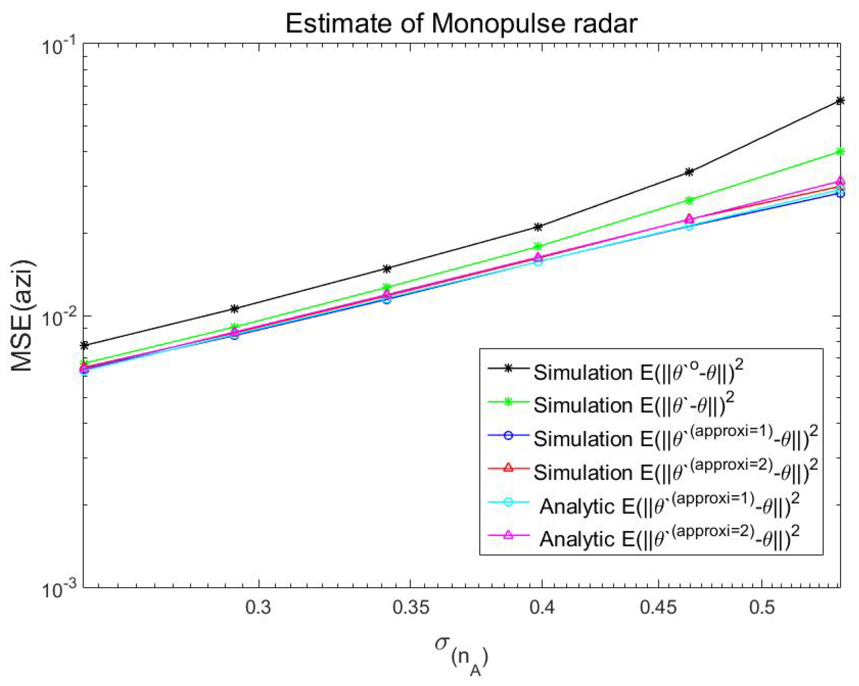
Table 1 tabulates various parameters of the simulation. The MSEs with respect to the standard derivation of an additive noise are illustrated in Figure 3 and Figure 4 for amplitude comparison monopulse radar.
The estimates used for getting ‘ Simulation E θ ¯ θ ¯ T 2 ’ in Figure 3 and Figure 4 are obtained from (15), and those for getting ‘ Simulation E θ ¯ θ ¯ T 2 ’ in Figure 3 and Figure 4 are obtained from (16) and (17). The estimates used for getting ‘ Simulation E θ ¯ ( approxi = 1 ) θ ¯ T 2 ’ in Figure 3 and Figure 4 are obtained from (18), and those for getting ‘ Simulation E θ ¯ ( approxi = 2 ) θ ¯ T 2 ’ in Figure 3 and Figure 4 are obtained from (19) and (20). Empirical MSEs of ‘ Simulation E θ ¯ o θ ¯ T 2 ’, ‘ Simulation E θ ¯ θ ¯ T 2 ’, ‘ Simulation E θ ¯ ( approxi = 1 ) θ ¯ T 2 ’ and ‘ Simulation E θ ¯ ( approxi = 2 ) θ ¯ T 2 ’ in Figure 3 and Figure 4 are calculated from (27). The results in Figure 3 and Figure 4 with ‘ Analytic E θ ¯ ( approxi = 1 ) θ ¯ T 2 ’ are obtained from (28), and those in Figure 3 and Figure 4 with ‘ Analytci E θ ¯ ( approxi = 2 ) θ ¯ T 2 ’ are obtained from (29) and (30). There is a little difference between ‘ Simulation E θ ¯ o θ ¯ T 2 ’ and ‘ Simulation E θ ¯ θ ¯ T 2 ’, because θ and ϕ are approximated estimates defined from the approximate antenna pattern. Note that θ o and ϕ o are true estimates defined from (3).
Also, ‘ Simulation E θ ¯ θ ¯ T 2 ’ is not equal to ‘ Simulation E θ ¯ ( approxi = 1 ) θ ¯ T 2 ’, as the first-order approximation is used to get ‘ Simulation E θ ¯ ( approxi = 1 ) θ ¯ T 2 ’ from ‘ Simulation E θ ¯ θ ¯ T 2 ’. Similarly, ‘ Simulation E θ ¯ θ ¯ T 2 ’ is not equal to ‘ Simulation E θ ¯ ( approxi = 2 ) θ ¯ T 2 ’, as the second-order approximation is used to get ‘ Simulation E θ ¯ ( approxi = 2 ) θ ¯ T 2 ’ from ‘ Simulation E θ ¯ θ ¯ T 2 ’. Noted that ‘ Simulation E θ ¯ ( approxi = 1 ) θ ¯ T 2 ’ and ‘ Analytic E θ ¯ ( approxi = 1 ) θ ¯ T 2 ’ show excellent agreements, which validates (5.8) with ‘ approxi = 1 ’. Also, ‘ Simulation E θ ¯ ( a p p r o x i = 2 ) θ ¯ T 2 ’ and ‘ Analytic E θ ¯ ( approxi = 2 ) θ ¯ T 2 ’ show excellent agreements, which validates (19) and (20) with ’ approxi = 2 ’. Therefore, the analytically derived expression ‘ Analytic E θ ¯ ( approxi = 1 ) θ ¯ T 2 ’ can be used to see how ‘ Simulation E θ ¯ ( approxi = 1 ) θ ¯ T 2 ’ is dependent on the standard deviation of an additive noise.
The results in Figure 3 and Figure 4 show that the MSEs of the angle estimate increase with the increase of SNR in the four antennas. Also, it is clear that the results with the superscript ‘ approxi = 2 ’ are much closer than the results with the superscript ‘ approxi = 1 ’ to the estimates without approximations.
Note that the proposed scheme is not a new DOA estimation algorithm with better MSE performance than previous existing DOA estimation algorithms. The proposed scheme is on how MSE of previously existing amplitude comparison monopulse DOA algorithm can be obtained analytically with much less computational complexity than the Monte Carlo simulation-based MSE. Therefore, we cannot quantitatively state how much improvement in estimation accuracy in terms of MSE can be achieved by adopting the proposed scheme in this paper.
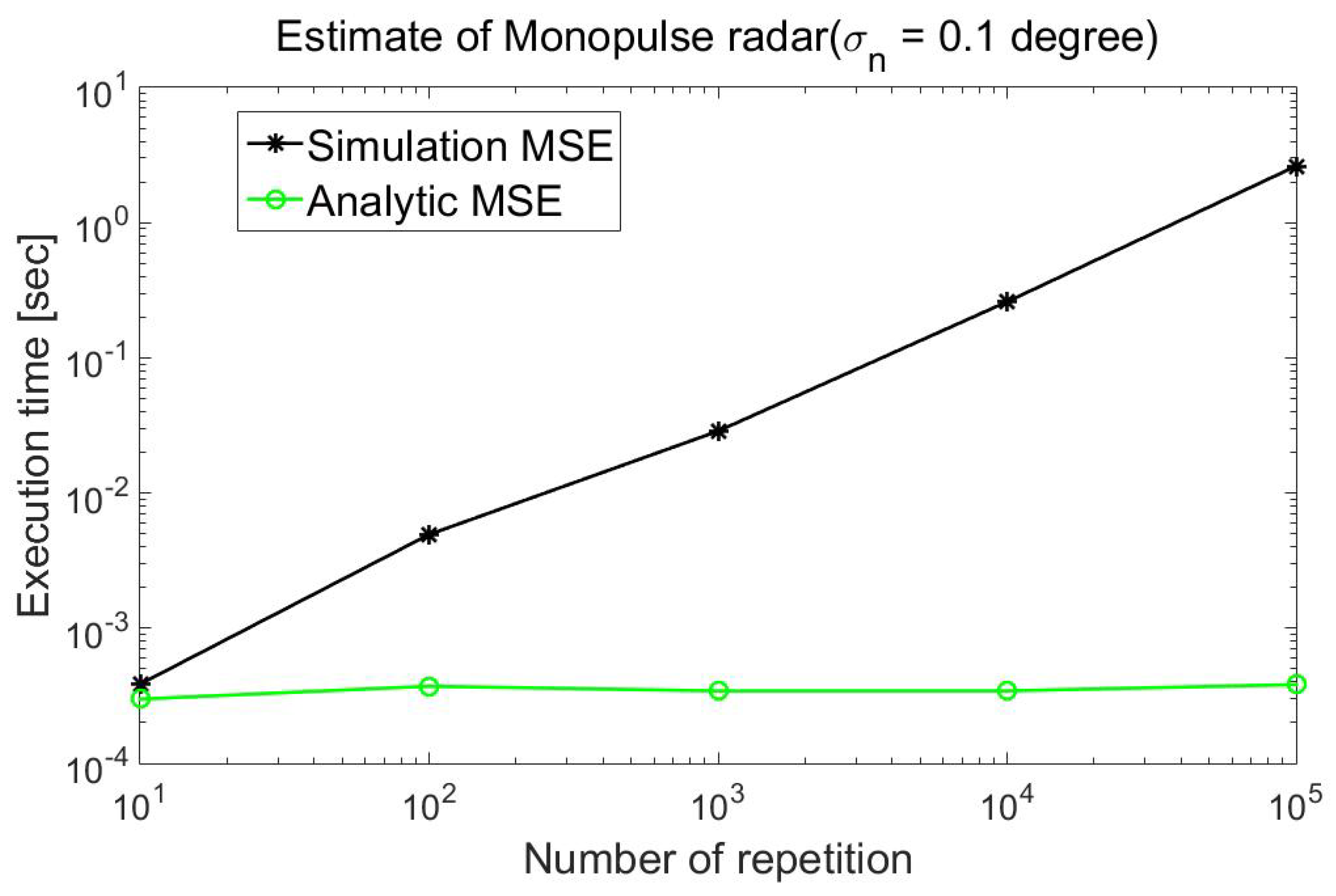
Instead, to quantify the improvement in the computational cost, computational complexity in execution time is illustrated both for analytically derived MSE and for the Monte Carlo simulation-based MSE. Note that the computational complexity is independent of the standard deviation. Therefore, the results for an arbitrary standard deviation of 0.1 degree is adopted for illustration.
As, in getting the Monte Carlo simulation-based MSE, the computational complexity is nearly proportional to the number of repetitions, the results for number of repetitions of 10, 100, 1000, 10,000 and 100,000 are shown. It is clearly shown in Figure 5 that the computational complexity for analytically derived MSE is much less than that for the Monte Carlo simulation-based MSE with number of repetitions = 100,000. Note that the execution time for analytically derived MSE is independent of the number of repetitions, which is why the execution time of the analytically derived MSE is flat with respect to the number of repetitions.

6. Conclusions

In this paper, monopulse radar was used to detect the angular error through a single pulse of the received signal. The tracking performance of the amplitude-comparison monopulse radar was analysed assuming that the signals received from the four antennas have different amplitudes from the same phase. Also, this paper deals with an analytic expression of the MSEs of the target angle estimate obtained from the approximation. The derivation is based on the assumption that additive noises of the measured angle components are Gaussian-distributed.
The usefulness of the derived expression is that the MSEs of the monopulse algorithm angle estimate using the different gain of received signal at array antenna can be available from the derived expression without actually performing the computationally intensive Monte Carlo simulation, which is illustrated in the numerical results. By using the derived expression, we can get a quantitative measure of how accurate the estimates are without actually performing the computationally intensive Monte Carlo simulation.
To quantify the computational reduction in getting the MSE analytically in comparison with the Monte Carlo simulation-based MSE, execution time with respect to the number of repetitions in the Monte Carlo simulation is illustrated in Figure 5, where the reduction in computational complexity associated with the analytically derived MSE in comparison with the Monte Carlo simulation-based MSE is clearly shown.

Author Contributions

D.-J.A. made a Matlab simulation and wrote the initial draft. J.-H.L. and D.-J.A. derived the mathematical formulation of the proposed scheme. In addition, J.-H.L. checked the numerical results and corrected the manuscript. All authors have read and agreed to the published version of the manuscript.

Funding

The authors gratefully acknowledge the support from Electronic Warfare Research Center (EWRC) at Gwangju Institute of Science and Technology (GIST), originally funded by Defense Acquisition Program Administration (DAPA) and Agency for Defense Development (ADD).

Conflicts of Interest

The authors declare no conflicts of interest.

Appendix A. The Explicit Expression of the MSEs Based on the Taylor Series

In this appendix, the received noise of four antenna— n A , n B , n C and n D —are defined as a normal distribution random variable. Generally, random variables n A , n B , n C and n D are distributed normally with mean μ and variance σ 2 [22].
n A N μ , σ 2 n B N μ , σ 2 n C N μ , σ 2 n D N μ , σ 2 .
Based on (A1), various statistics in (A2) and (A3) can be obtained:
E n k n l = E [ n k 2 ] k = l E [ n k ] E [ n l ] otherwise
E n A = μ E n A 2 = μ 2 + σ A 2 E n A 3 = μ 3 + 3 μ σ A 2 E n A 4 = μ 4 + 6 μ 2 σ A 2 + 3 σ A 4
For brevity, α A , α B , α C , α D , β A , β B , β C , β D , β A B , β A C , β A D , β B C , β B D and β C D are defined from the expressions in (28):
α A = α D = θ 3 d B θ 3 d B k m k m θ ¯ T 4 A G 0 , α B = α C = θ 3 d B θ 3 d B k m k m + θ ¯ T 4 A G 0 , β A = β D = 2 θ 3 d B θ 3 d B k m k m θ ¯ T 4 A G 0 2 , β B = β C = 2 θ 3 d B θ 3 d B k m k m + θ ¯ T 4 A G 0 2 , β A B = β A C = β B D = β C D = 2 θ ¯ T 4 A G 0 2 , β A D = β A , β B C = β B .
Using (A1)–(A4), the explicit expressions of MSEs are expressed as (A5)–(A8)
E θ ^ approxi = 1 θ 2 = E n A 2 α A 2 + E n B 2 α B 2 + E n C 2 α C 2 + E n D 2 α D 2 + 2 E n A n B α A α B + 2 E n A n C α A α C + 2 E n A n D α A α D + 2 E n B n C α B α C + 2 E n B n D α B α D + 2 E n C n D α C α D + E n A α A + E n B α B + E n C α C + E n D α D 2 = μ 2 + σ A 2 α A 2 + μ 2 + σ B 2 α B 2 + μ 2 + σ C 2 α C 2 + μ 2 + σ D 2 α D 2 + 2 μ 2 α A α B + 2 μ 2 α A α C + 2 μ 2 α A α D + 2 μ 2 α B α C + 2 μ 2 α B α D + 2 μ 2 α C α D + μ α A + μ α B + μ α C + μ α D 2 .
E ϕ ^ approxi = 1 ϕ 2 = E n A 2 α A 2 + E n D 2 α B 2 + E n C 2 α C 2 + E n B 2 α D 2 + 2 E n A n D α A α B + 2 E n A n C α A α C + 2 E n A n B α A α D + 2 E n D n C α B α C + 2 E n B n D α B α D + 2 E n C n B α C α D + E n A α A + E n D α B + E n C α C + E n B α D 2 = μ 2 + σ A 2 α A 2 + μ 2 + σ D 2 α B 2 + μ 2 + σ C 2 α C 2 + μ 2 + σ B 2 α D 2 + 2 μ 2 α A α B + 2 μ 2 α A α C + 2 μ 2 α A α D + 2 μ 2 α B α C + 2 μ 2 α B α D + 2 μ 2 α C α D + μ α A + μ α B + μ α C + μ α D 2 .
E θ ^ a p p r o x i = 2 θ 2 = μ 2 + σ A 2 α A 2 + μ 2 + σ B 2 α B 2 + μ 2 + σ C 2 α C 2 + μ 2 + σ D 2 α D 2 + μ 4 + 6 μ 2 σ A 2 + 3 σ A 4 4 β A 2 + μ 4 + 6 μ 2 σ B 2 + 3 σ B 4 4 β B 2 + μ 4 + 6 μ 2 σ C 2 + 3 σ C 4 4 β C 2 + μ 4 + 6 μ 2 σ D 2 + 3 σ D 4 4 β D 2 + μ 2 + σ A 2 μ 2 + σ B 2 β A B 2 + μ 2 + σ A 2 μ 2 + σ C 2 β A C 2 + μ 2 + σ A 2 μ 2 + σ D 2 β A D 2 + μ 2 + σ B 2 μ 2 + σ C 2 β B C 2 + μ 2 + σ B 2 μ 2 + σ D 2 β B D 2 + μ 2 + σ C 2 μ 2 + σ D 2 β C D 2 + 2 μ 2 α A α B + 2 μ 2 α A α C + 2 μ 2 α A α D + 2 μ 2 α B α C + 2 μ 2 α B α D + 2 μ 2 α C α D + 1 2 μ 2 + σ A 2 μ 2 + σ B 2 β A β B + 1 2 μ 2 + σ A 2 μ 2 + σ C 2 β A β C + 1 2 μ 2 + σ A 2 μ 2 + σ D 2 β A β D + 1 2 μ 2 + σ B 2 μ 2 + σ C 2 β B β C + 1 2 μ 2 + σ B 2 μ 2 + σ C 2 β B β C + 1 2 μ 2 + σ C 2 μ 2 + σ D 2 β C β D + 2 μ 2 + σ A 2 μ 2 β A B β A C + 2 μ 2 + σ A 2 μ 2 β A B β A D + 2 μ 2 + σ B 2 μ 2 β A B β B C + 2 μ 2 + σ B 2 μ 2 β A B β B D + 2 μ 4 β A B β C D + 2 μ 2 + σ A 2 μ 2 β A C β A D + 2 μ 2 + σ C 2 μ 2 β A C β B C + 2 μ 4 β A C β B D + 2 μ 2 + σ C 2 μ 2 β A C β C D + 2 μ 4 β A D β B C + 2 μ 2 + σ C 2 μ 2 β A D β B D + 2 μ 2 + σ D 2 μ 2 β A D β C D + 2 μ 2 + σ B 2 μ 2 β B C β B D + 2 μ 2 + σ C 2 μ 2 β B C β C D + 2 μ 2 + σ D 2 μ 2 β B D β C D + 2 μ α A + μ α B + μ α C + μ α D μ 2 + σ A 2 2 β A + μ 2 + σ B 2 2 β B + μ 2 + σ C 2 2 β C + μ 2 + σ D 2 2 β D + 2 μ α A + μ α B + μ α C + μ α D μ 2 β A B + μ 2 β A C + μ 2 β A D + μ 2 β B C + μ 2 β B D + μ 2 β C D + 2 μ 2 + σ A 2 2 β A + μ 2 + σ B 2 2 β B + μ 2 + σ C 2 2 β C + μ 2 + σ D 2 2 β D μ 2 β A B + μ 2 β A C + μ 2 β A D + μ 2 β B C + μ 2 β B D + μ 2 β C D .
E ϕ ^ a p p r o x i = 2 ϕ 2 = μ 2 + σ A 2 α A 2 + μ 2 + σ D 2 α B 2 + μ 2 + σ C 2 α C 2 + μ 2 + σ B 2 α D 2 + μ 4 + 6 μ 2 σ A 2 + 3 σ A 4 4 β A 2 + μ 4 + 6 μ 2 σ D 2 + 3 σ D 4 4 β B 2 + μ 4 + 6 μ 2 σ C 2 + 3 σ C 4 4 β C 2 + μ 4 + 6 μ 2 σ B 2 + 3 σ B 4 4 β D 2 + μ 2 + σ A 2 μ 2 + σ D 2 β A B 2 + μ 2 + σ A 2 μ 2 + σ C 2 β A C 2 + μ 2 + σ A 2 μ 2 + σ B 2 β A D 2 + μ 2 + σ D 2 μ 2 + σ C 2 β B C 2 + μ 2 + σ B 2 μ 2 + σ D 2 β B D 2 + μ 2 + σ C 2 μ 2 + σ B 2 β C D 2 + 2 μ 2 α A α B + 2 μ 2 α A α C + 2 μ 2 α A α D + 2 μ 2 α B α C + 2 μ 2 α B α D + 2 μ 2 α C α D + 1 2 μ 2 + σ A 2 μ 2 + σ D 2 β A β B + 1 2 μ 2 + σ A 2 μ 2 + σ C 2 β A β C + 1 2 μ 2 + σ A 2 μ 2 + σ B 2 β A β D + 1 2 μ 2 + σ D 2 μ 2 + σ C 2 β B β C + 1 2 μ 2 + σ D 2 μ 2 + σ C 2 β B β C + 1 2 μ 2 + σ C 2 μ 2 + σ B 2 β C β D + 2 μ 2 + σ A 2 μ 2 β A B β A C + 2 μ 2 + σ A 2 μ 2 β A B β A D + 2 μ 2 + σ D 2 μ 2 β A B β B C + 2 μ 2 + σ D 2 μ 2 β A B β B D + 2 μ 4 β A B β C D + 2 μ 2 + σ A 2 μ 2 β A C β A D + 2 μ 2 + σ C 2 μ 2 β A C β B C + 2 μ 4 β A C β B D + 2 μ 2 + σ C 2 μ 2 β A C β C D + 2 μ 4 β A D β B C + 2 μ 2 + σ C 2 μ 2 β A D β B D + 2 μ 2 + σ B 2 μ 2 β A D β C D + 2 μ 2 + σ D 2 μ 2 β B C β B D + 2 μ 2 + σ C 2 μ 2 β B C β C D + 2 μ 2 + σ B 2 μ 2 β B D β C D + 2 μ α A + μ α B + μ α C + μ α D μ 2 + σ A 2 2 β A + μ 2 + σ D 2 2 β B + μ 2 + σ C 2 2 β C + μ 2 + σ B 2 2 β D + 2 μ α A + μ α B + μ α C + μ α D μ 2 β A B + μ 2 β A C + μ 2 β A D + μ 2 β B C + μ 2 β B D + μ 2 β C D + 2 μ 2 + σ A 2 2 β A + μ 2 + σ D 2 2 β B + μ 2 + σ C 2 2 β C + μ 2 + σ B 2 2 β D μ 2 β A B + μ 2 β A C + μ 2 β A D + μ 2 β B C + μ 2 β B D + μ 2 β C D .

Appendix B. The Explicit Expression of the MSEs Based on the Taylor Series for Zero-Mean Noises

In this appendix, the received noise of four antenna— n A , n B , n C and n D —are defined as a normal distribution random variable. Generally, random variables n A , n B , n C and n D are distributed normally with mean 0 and variance σ 2 [22].
n A N 0 , σ 2 n B N 0 , σ 2 n C N 0 , σ 2 n D N 0 , σ 2 .
Based on (A9), various statistics in (A10) and (A11) can be obtained:
E n k n l = E [ n k 2 ] k = l E [ n k ] E [ n l ] = 0 otherwise
E n A = 0 E n A 2 = σ A 2 E n A 3 = 0 E n A 4 = 3 σ A 4 .
For brevity, α A , α B , α C , α D , β A , β B , β C , β D , β A B , β A C , β A D , β B C , β B D and β C D are defined from the expressions in (28):
α A = α D = θ 3 d B θ 3 d B k m k m θ ¯ T 4 A G 0 , α B = α C = θ 3 d B θ 3 d B k m k m + θ ¯ T 4 A G 0 , β A = β D = 2 θ 3 d B θ 3 d B k m k m θ ¯ T 4 A G 0 2 , β B = β C = 2 θ 3 d B θ 3 d B k m k m + θ ¯ T 4 A G 0 2 , β A B = β A C = β B D = β C D = 2 θ ¯ T 4 A G 0 2 , β A D = β A , β B C = β B .
Using (A9)–(A12), the explicit expressions of MSEs are expressed as (A13)–(A16).
E θ ^ approxi = 1 θ 2 = E n A 2 α A 2 + E n B 2 α B 2 + E n C 2 α C 2 + E n D 2 α D 2 = σ A 2 α A 2 + σ B 2 α B 2 + σ C 2 α C 2 + σ D 2 α D 2 .
E ϕ ^ approxi = 1 ϕ 2 = E n A 2 α A 2 + E n D 2 α B 2 + E n C 2 α C 2 + E n B 2 α D 2 = σ A 2 α A 2 + σ D 2 α B 2 + σ C 2 α C 2 + σ B 2 α D 2 .
E θ ^ a p p r o x i = 2 θ 2 = σ A 2 α A 2 + σ B 2 α B 2 + σ C 2 α C 2 + σ D 2 α D 2 + 3 σ A 4 4 β A 2 + 3 σ B 4 4 β B 2 + 3 σ C 4 4 β C 2 + 3 σ D 4 4 β D 2 + σ A 2 σ B 2 β A B 2 + σ A 2 σ C 2 β A C 2 + σ A 2 σ D 2 β A D 2 + σ B 2 σ C 2 β B C 2 + σ B 2 σ D 2 β B D 2 + σ C 2 σ D 2 β C D 2 + 1 2 σ A 2 σ B 2 β A β B + 1 2 σ A 2 σ C 2 β A β C + 1 2 σ A 2 σ D 2 β A β D + 1 2 σ B 2 σ C 2 β B β C + 1 2 σ B 2 σ C 2 β B β C + 1 2 σ C 2 σ D 2 β C β D .
E ϕ ^ a p p r o x i = 2 ϕ 2 = σ A 2 α A 2 + σ D 2 α B 2 + σ C 2 α C 2 + σ B 2 α D 2 + 3 σ A 4 4 β A 2 + 3 σ D 4 4 β B 2 + 3 σ C 4 4 β C 2 + 3 σ B 4 4 β D 2 + σ A 2 σ D 2 β A B 2 + σ A 2 σ C 2 β A C 2 + σ A 2 σ B 2 β A D 2 + σ D 2 σ C 2 β B C 2 + σ B 2 σ D 2 β B D 2 + σ C 2 σ B 2 β C D 2 + 1 2 σ A 2 σ D 2 β A β B + 1 2 σ A 2 σ C 2 β A β C + 1 2 σ A 2 σ B 2 β A β D + 1 2 σ D 2 σ C 2 β B β C + 1 2 σ D 2 σ C 2 β B β C + 1 2 σ C 2 σ B 2 β C β D .

References

  1. Rhodes, D.R. Introduction to Monopulse; Artech House: Boston, MA, USA, 1980. [Google Scholar]
  2. Sherman, S.M. Monopulse Principles and Techniques; Artech House: Boston, MA, USA, 1984. [Google Scholar]
  3. Sherman, S.M.; Barton, D.K. Monopulse Principles and Techniques, 2nd ed.; Artech House: Pacific Grove, CA, USA, 2011; Volume 1, pp. 295–299. [Google Scholar]
  4. Leonov, A.I.; Fomichev, K.I. Monopulse Radar; National Technical Information Service: Alexandria, VA, USA, 1972. [Google Scholar]
  5. Leonov, A.I.; Fomichev, K.I. Monopulse Radar; Barton, W.F., Ed.; Artech House: Boston, MA, USA, 1986. [Google Scholar]
  6. Dunn, J.H.; Howard, D.D.; Pendleton, K.B. Tracking radar. In Radar Handbook; Skolnik, M.I., Ed.; McGraw-Hill: New York, NY, USA, 1970; Chapter 21; pp. 71–78. [Google Scholar]
  7. Hofstetter, E.; DeLong, D. Detection and parameter estimation in an amplitude-comparison monopulse radar. IEEE Trans. Inf. Theory 1969, 15, 22–30. [Google Scholar] [CrossRef]
  8. Adams, R.N.; Horowitz, L.L.; Senne, K.D. Adaptive main-beam nulling for narrow-beam antenna arrays. IEEE Trans. Aerosp. Electron. Syst. 1980, AES-16, 509–516. [Google Scholar] [CrossRef]
  9. Davis, R.C.; Brennan, L.E.; Reed, L.S. Angle estimation with adaptive arrays in external noise fields. IEEE Trans. Aerosp. Electron. Syst. 1976, AES-12, 179–186. [Google Scholar] [CrossRef]
  10. Yoganandam, Y.; Das, R.J. Performance analysis of a noncoherent monopulse processor in the presence of target glint and receiver imbalances. IEE Proc. F (Radar Signal Process.) 1991, 138, 445–452. [Google Scholar] [CrossRef]
  11. Zheng, Y.; Tseng, S.-M.; Yu, K.-B. Closed-form four-channel monopulse two-target resolution. IEEE Trans. Aerosp. Electron. Syst. 2016, 39, 1083–1089. [Google Scholar] [CrossRef]
  12. Chen, L.; Sheng, W. Performance analysis for angle measurement of monopulse radar with non-consistent amplitude-phase features. In Proceedings of the 2010 International Conference on Microwave and Millimeter Wave Technology, Chengdu, China, 8–11 May 2010. [Google Scholar]
  13. Jacovitti, G. Performance analysis of monopulse receivers for secondary surveillance radar. IEEE Trans. Aerosp. Electron. Syst. 1983, AES-19, 884–897. [Google Scholar] [CrossRef]
  14. Paine, A.S. Minimum variance monopulse technique for an adaptive phased array radar. IEE Proc. Radar Sonar Navig. 1998, 145, 374–380. [Google Scholar] [CrossRef]
  15. Nickel, U. Monopulse estimation with adaptive arrays. IEE Proc. F (Radar Signal Process.) 1993, 140, 303–308. [Google Scholar] [CrossRef]
  16. Nickel, U. Monopulse estimation with subarray-adaptive arrays and arbitrary sum and difference beams. IEE Proc. Radar Sonar Navig. 1996, 143, 232–238. [Google Scholar] [CrossRef]
  17. Song, S. Performance Analysis Angle Tracking Using Adaptive Kalman Filter in Monopulse Radar. Master’s Thesis, Jeju University, Jeju, Korea, 2017. [Google Scholar]
  18. Choi, J.-I.; Kim, S.-W.; Chin, H.-C.; Choi, W.-H. A study on the improvement of direction error for electronic warfare system. Korea Acad. Ind. Coop. Soc. 2017, 18, 567–575. [Google Scholar]
  19. Sim, H.-K.; Jung, M.-A.; Kim, S.-C. A performance analysis of phase comparison monopulse algorithm for antenna spacing and antenna array. J. Korean Inst. Commun. Inf. Sci. 2015, 40, 1413–1419. [Google Scholar] [CrossRef] [Green Version]
  20. Cho, B.-L.; Lee, J.-S.; Lee, J.-M.; Sun, S.-G. Accuracy improvement of the estimated angle using phase averaging in phase-comparison monopulse algorithm. J. Korean Inst. Electromagn. Eng. Sci. 2012, 23, 1212–1215. [Google Scholar] [CrossRef]
  21. Han, Y.J.; Kim, J.W.; Park, S.R.; Noh, S. An investigation into the monopulse radar using tx-rx simulator in electronic warfare settings. In Proceedings of the Symposium of the Korean Institute of communications and Information Sciences, Jeongseon, Korea, 19 January 2017; pp. 705–706. [Google Scholar]
  22. Normal Distribution. Available online: https://en.wikipedia.org/wiki/Normaldistribution (accessed on 10 February 2020).
Figure 1. Illustration of monopulse concept.
Applsci 10 01246 g001
Figure 2. Track axis and angular error of monopulse radar beam.
Applsci 10 01246 g002
Figure 3. Mean square errors (MSEs) of target azimuth estimate for ACM radar.
Applsci 10 01246 g003
Figure 4. MSEs of target elevation estimate for ACM radar.
Applsci 10 01246 g004
Figure 5. Execution time of MSEs of target estimate for ACM radar.
Applsci 10 01246 g005
Table 1. Parameters for simulation.
DescriptionValueUnits
Monte Carlo simulation100,000times
The mean of the noise received at Antenna A, B, C, D0voltage/meter
The standard deviation of the noise received at Antenna A, B, C, D 10 0.6 , 10 0.5 , , 10 0 degrees
Antenna 3 dB beamwidth3degrees
Track axis gain1voltage
Antenna squint angle1degrees
Gain of received signal1voltage

