1. Introduction
Changeable and severe environment is the main cause of failures for wind turbines (WT), such frequent malfunctions will inevitably lead to low availability and expensive maintenance costs [
1]. In general, various types of condition monitoring sensors are installed in different WT components, and their multi-dimensional state parameters, such as wind speed, pitch angle, hydraulic oil temperature, etc., are recorded and saved by the WT supervisory control and data acquisition (SCADA) system [
2]. Once an exception occurs, its fault information will be fed back in the multi-dimensional sensor parameters of the SCADA system [
3], where such parameters are referred as “SCADA data”. Hence, using the SCADA data for early anomaly detection is beneficial to achieve the condition assessment and fault warning of wind turbines.
Generally, fault detection and isolation (FDI) approaches have two critical processes: (1) Extract effective features from the complex data, and (2) use prior knowledge or machine learning techniques to achieve failure classifications. It is worth noting that both steps need obvious label information (normal or abnormal labels) as the essential elements of training the intelligent classification algorithms [
4,
5]. But in the actual WT operation, it is almost impossible to acquire enough label data. This is because the normal operation time is much longer than fault occurrence time, which causes the data sparseness to be inevitable. In addition, the monitoring data and fault information of the SCADA system are mostly recorded separately, and the correlation between them only depends on manual completion after the fault occurs. Such non-intelligent recording and classifying work is huge and unrealistic. Therefore, using imperfect labels to complete FDI of the wind turbines is fraught with challenges.
Deep learning methods [
6] have been widely reported in data mining and intelligent fault diagnosis due to their excellent nonlinear approximation performance [
7]. Compared with the shallow neural networks, the deep learning algorithms [
8], such as multi-layer perceptron (MLP), deep neural network (DNN), long short-term memory (LSTM) or convolutional neural network (CNN), can mine valuable information from the data more truly and effectively through the real imitation of the human learning process. Jiang and He [
9] proposed a multi-scale convolutional neural network to effectively learn the high-level fault features and obtain rich diagnostic information on different vibration frequencies. Yang et al. used the LSTM-based recurrent neural network (RNN) to mine the spatial or temporal relationships hidden in SCADA signals, so as to realize the fault classification of WT gears [
10]. Faced with a large amount of textual data collected in the SCADA system, recent research work has innovatively transformed them into image or map form and then used image recognition algorithms to detect and identify anomalies. For instance, Yu et al. converted the vibration signal into time-domain spectrums, and then applied the CNN to extract the fault features [
11]. Du [
12] first arranged the multidimensional SCADA data and then used a window function to slide to intercept a digital matrix of equal length and width. Each value in this digital matrix is equivalent to the pixel value in an image. On this basis, the multilayer CNN is used for deep-level anomaly detection. The methods mentioned above provide more possibilities for the realization of WT fault diagnosis. However, the implementation of the above networks requires a supervised learning environment with sufficient labels, which is a gap and difficult to achieve in practical applications.
The techniques of using unsupervised learning in FDI are also relatively mature. The corresponding algorithms are mainly deep learning networks [
13] constructed with Restricted Boltzmann Machine (RBM) or Auto-encoder (AE). Deep belief network (DBN) [
14], denoise auto-encoder (DAE) [
15], and stacked auto-encoder (SAE) [
16] are the most representative unsupervised deep learning networks. In the field of fault diagnosis, auto-encoder is the most widely used. The process of the auto-encoder is to first explore the fusion rules of hidden features from the unlabeled input data by encoding, and then interpret the hidden features through decoding to give a more prominent output than the original data. Qin [
17] used a DBN to diagnose the fault of the planetary gearbox in wind turbines and proposed an improved Logistic-sigmoid unit and pulse characteristic method to solve the problem that DBN is prone to gradient disappearance in the back propagation. Bai and Qin built a deep-stacked auto-encoder network based on a multilayer back propagation (BP) neural network [
18]. First, the SAE network neurons are trained layer by layer through unsupervised greedy learning by using the bearing data collected from the SCADA system. Then the trained weights are used as the initial weights of the deep BP neural network, and the labeled data, in a supervised manner, to continue training the network. In addition, Zhao proposed a deep auto-encoder network based on multiple RBMs to implement early abnormality detection and fault detection of wind turbine components [
19].
However, deep learning networks with different structures are not born equal, one kind of network for specific tasks may be superior to others. For example, a convolution neural network is suitable for image recognition, while the recurrent neural network is adept in speech analyzing. Hence the structures of the neural networks will be improved with the changing application field. At present, the improved methods for neural networks mainly include deepening network level, dropout and drop-connect, batch normalization, and so on. Among them, increasing the connection edges between non-adjacent hidden layers (add-edge) is the current research focus of neural networks to alleviate gradient disappearance. From the view of network structure, the add-edge improvement makes the traditional neural network become a small-world neural network, which is a middle topology between regularity and disorder. The authors of this paper have improved a BP neural network into a small-world one and then used it to predict the wind power [
20]. On this basis, a selective ensemble strategy combining multiple small-world neural networks has been proposed to diagnose and detect the WT pitch failures [
21]. Combined with the characteristics of wind turbines’ SCADA data, this paper proposed a deep small-world neural network (DSWNN) for anomaly detection of wind turbines. First, a DSWNN prototype using multiple restricted Boltzmann machines (RBM) was constructed based on the classical deep auto-encoder network. Previously unlabeled SCADA data from wind turbines were used to pre-train this DSWNN prototype to extract implied features. Then, the regular neural network was transformed into a small-world one though a randomly add-edge method, and the labeled data were used to train the reconstructed DSWNN model within the supervised case to fine-tune the global parameters of the network. Due to the acute changes and disturbances of wind speed in actual operation, the fixed thresholds for judging failures are always unreasonable and can cause false alarms. Therefore, an adaptive threshold determined by extreme value theory was presented as the criterion of anomaly judgment. Finally, the effectiveness of the proposed method was verified by two failure cases of wind turbine pitch systems.
The remainder of this paper is organized as follows.
Section 2 describes the proposed DSWNN model and its training method;
Section 3 gives the estimating method of the adaptive threshold;
Section 4 presents and discusses two failure cases of wind turbine pitch system. Finally,
Section 5 lists the conclusion of the study. All abbreviations and symbols used in this paper are shown in
Table A1 and
Table A2 of the
Appendix A.
2. Deep Small-World Neural Network (DSWNN)
A deep auto-encoder network is a deep learning network with multiple hidden layers between the input and out layers, which can model complex non-linear relationships among multiple types of variables. The parameters of this network are initialized by unsupervised learning for input data layer by layer, and then supervised learning is used for fine-tuning. In this network framework, deep learning models lead to more complex features at higher output layers, and the learned complex features will be invariant with the change of input data [
22,
23]. In this paper, the proposed DSWNN model is an improved deep auto-encoder network that has small-world characteristics. Such improvement adds additional neuron connections between non-adjacent hidden layers on the basis of the original network structure. In particular, the DSWNN model is composed of multiple RBM stacks, and
Figure 1 gives an example of the DSWNN structure with four hidden layers. The training process of the DSWNN model includes three phases, pre-training, small-world transformation and fine-tuning, which are applied to obtain the model parameters.
2.1. Pre-Training of the DSWNN Prototype
As mentioned above, the DSWNN prototype is a deep auto-encoder network with multiple RBMs. An RBM is a specific energy-based stochastic model [
24] with one visible layer and one hidden layer, in which the visible neurons
v = (
v1,
v2,…,
vm) are connected fully to the hidden neurons
h = (
h1,
h2,…,
hn).
Figure 2 shows the mechanisms of an RBM.
In the RBM, the energy of the joint configuration units
E(
v,
h) is shown as Equation (1), and the joint probability
P(
v,
h) between units based on the energy model is described as Equation (2).
where
wij is the symmetric weight between visible neurons
i and hidden neurons
j,
vi,
hj are the binary states and
ai,
bj are their biases, respectively. The unbiased samples of
vi and
hj give a hidden vector
h and a visible vector
v can be calculated as follows:
where
f(•) is an activation function that can be taken as a logistic Sigmoid function or
tanh function, which are defined as Equation (5).
The essence of the activation function is to retain the characteristics of the activated neuron and map it out. The derivative of the log-likelihood with respect to weight
wij is shown in Equation (6).
where, 〈
vihj〉
data represents the expectation with respect to the data distribution, and 〈
vihj〉
model represents the expectation with respect to the model distribution.
However, getting an accurate description of 〈
vihj〉
model is computationally intractable, so Hinton proposed a Contrastive Divergence (CD) algorithm to crudely approximate the gradient [
25]. First, the CD algorithm uses the input data to initialize the visible layer, and then calculates the hidden layer based on conditional distribution rules. Second, the visible layer is also calculated according to the hidden layer. Relying on the repeated calculation, a reconstruction of the input data is obtained.
where,
η is the learning rate, 〈
vihj〉
recon is the expectation of reconstruction states, which is calculated by Gibbs sampler based on the initialized input data.
The DSWNN prototype needs to pre-trained first, which is regarded as the process of training multiple RBMs layer by layer. The output of each RBM is considered as a new input of another RBM with a higher level to achieve the transmission of learning results. Once an RBM is trained, the weights between two-layer neurons are determined and locked. This procedure is conducted in an unsupervised environment, and the whole network weights will be obtained after the layer by layer pre-training. These weights will be recorded and used as the prior values for subsequent supervised training (fine-tuning).
2.2. Small-World Transformation of DSWNN
A small-world network is an intermediate network between completely random and completely regular, which was originally proposed by Watts in 1998 to describe the natural distribution of biological, technological and social networks [
26]. After that, various researches began to apply the characteristics of a small-world network to the structural improvement of artificial neural networks (ANNs) [
21,
22,
27]. We summarize the current researches and consider that the small-world transformation has two ways (see
Figure 3): reconstruct-edge transformation and add-edge transformation.
Taking a four-layer BP neural network with four neurons in each layer as an example, the reconstruct-edge transformation first separates the connections between adjacent-layer neurons randomly, and then reconstructs the new connections between nonadjacent-layer neurons. The add-edge transformation does not have the disconnecting procedure, it only adds new connections between nonadjacent-layer neurons without changing any original edges. The positions of the newly added connections are all randomly distributed among all network neurons, and the degree of network randomization is described by probability
p.
where,
nad and
nor are the number of the newly added connections and original connections, respectively.
Figure 4 gives the random add-edge procedure from a regular network to a random one. When
p = 0 or
p = 1, the network is completely regular or completely random. While when
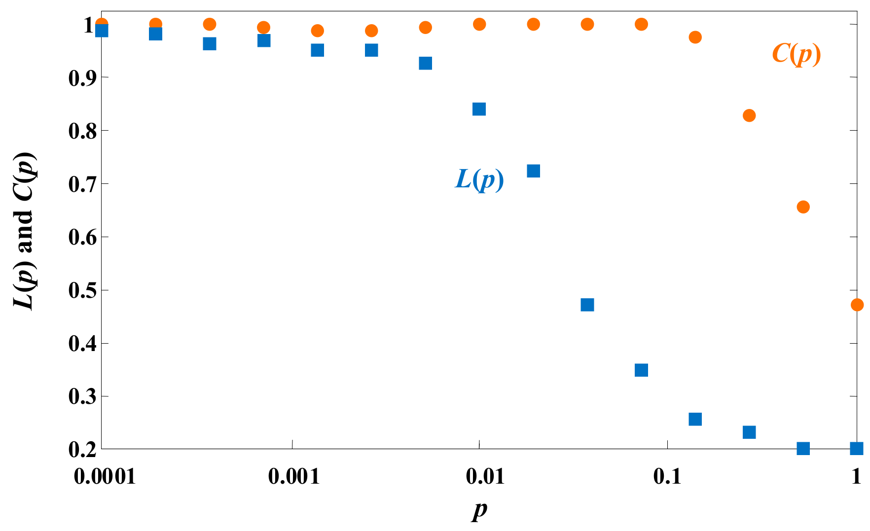
p is between 0 and 1, the network has a small-world property. To probe the intermediate region 0 <
p < 1, the characteristic path length
L(
p) and clustering coefficient
C(
p) are used to quantify the small world structural properties.
The characteristic path length
L(
p) is a global property of measuring the average length of all connected edges in a network, and clustering coefficient
C(
p) is a local property that is used to describe the density of connected edges in local areas.
Figure 5 shows the changing normalized values of
L(
p) and
C(
p) with
p for the four-hidden-layer DSWNN described in
Figure 1. It can be observed that as
p increases,
L(
p) drops sharply while
C(
p) descends relatively slowly. When
p moves towards 0.1, a large
C(
p) and a small
L(
p) are obtained, which indicates that the topology of the DSWNN has the best small-world properties. Therefore, the number of newly added edge connections is
p = 0.1 times of the total number of connections.
This paper selects the way of add-edge transformation to reconstruct the DSWNN model. Suppose that the DSWNN model has
H (
H = 1, 2, 3,…,
i,…) hidden layers, and there are
N neurons in the
ith hidden layer and
M neurons in the
i + 1th hidden layer. When
p = 0, the DSWNN model is a regular network and the weight matrix
Wi between the
ith and
i + 1th hidden layers is described as Equation (9). Accordingly, the connection matrix
W for the entire hidden layers can be expressed as in Equation (10).
When
p = 0.1, the DSWNN does not disconnect connections in the original network and only generates connections between neurons in the non-adjacent hidden layers. The diagonal weights in matrix
W are not changed because the connection does not disconnect. The global
Wa for the entire hidden layers can be represented as the Equation (11).
where,
is the weight matrix of the added edges between layer
a and layer
b, and its structure is shown in Equation (12).
where,
is the weight of the added edge between the
xth neuron in layer
a and the
yth neuron in layer
b.
N and
M represent the number of neurons contained in layers
a and
b, respectively.
On the basis of the probability p, the is a sparse matrix in which only the non-zero weights represent the randomly added edges. Therefore, transforming the DSWNN model into a small-world one is equivalent to randomly selecting the position in the global weight matrix and giving non-zero value. The pre-trained weights will not be changed in this procedure.
2.3. Fine-Tuning of the DSWNN Parameters
After the layer-wise pre-training and add-edge small-world transformation, the DSWNN model will be fine-tuned by using BP algorithm. BP is a classical method commonly used for supervised learning to improve the representation of data features and optimize the parameters of hidden layers in the fine-tuning. In this process, the initial parameters of the DSWNN model are composed of the pre-training parameters (weights and bias) and the edge-weights obtained by the small-world transformation. Because the fine-tuning only completes the local search based on these superior initial parameters, the convergence time of the optimization is significantly shortened in this process. After fine-tuning, the globally optimized parameters of the DSWNN model are obtained.
In this paper, the
tanh function is regarded as the activation function for hidden layers, and the Softmax as the activation function for the top classifier layer. Moreover, the Cross Entropy [
28] shown in Equation (13) is chosen as the cost function
C to measure error.
where,
k is the number of neurons in the output layer,
t is the expected output.
To summarize, the training process of the DSWNN model includes three steps.
- (1)
Pre-training: In the unsupervised case, each RBM of DSWNN is trained one by one to mine the feature information of the unlabeled input data.
- (2)
Small-world transformation: Lock the weight values obtained by pre-training, add new edges according to the probability p, and randomly assign the weight values to the newly added edges.
- (3)
Fine-tuning: Add a classification layer in the last layer of DSWNN to receive the output eigenvector from the last RBM. Train the entity DSWNN model with labeled data in the supervised case and the network global weights are adjusted by the BP algorithm.
Figure 6 gives the three training processes of the DSWNN model. The process of RBM training can be regarded as the initialization of the weight parameters for the DSWNN model, which overcomes the shortcomings of the network easily falling into local optimum and long training time due to the random initialization of the weight parameters. For the detection of WT abnormality, a large number of unlabeled SCADA data can be used for pre-training, and a small number of labeled data can be used for fine-tuning. In this way, the trained DSWNN is more optimized than the deep auto-encoder network or BP network alone.
3. Anomaly Detection Based on Adaptive Threshold Estimating Method
In anomaly detection, the trained DSWNN model is used to predict the future values of the SCADA signals, and the prediction error (
PE) between predicted value and actual value is used to judge the abnormalities. The
PE is defined as Equation (14).
where
X is the actual value of SCADA data, and
is the output of the DSWNN model.
Generally, setting a threshold and comparing it with the
PE is the most common and effective way to evaluate whether the wind turbine is in failure. When a wind turbine operates normally, the SCADA signals are all within the threshold range. Once an abnormality occurs, the implicit relationship between these monitoring signals will be broken, and one or more signal values will suddenly exceed the threshold to give an alarm. The rule for determining the abnormal condition is defined as Equation (15):
where
Rth is the threshold.
However, the thresholds are often set in a wide range and remain unchanged after one set. On the one hand, the faults within the threshold will not be diagnosed; on the other hand, some occasional fluctuations caused by the random wind speed will be misdiagnosed as faults. Therefore, this paper presents an adaptive threshold estimating method on the basis of the extreme value theory to monitor the trend of PE and detect its anomaly variation.
Suppose
X1,
X2,…,
Xn are
n sample vectors of independent and randomly distributed variables whose distribution function is
F(
x). Each sample vector of
Xi contains a certain amount of values in a period of time.
Mn = max(
X1,
X2,…,
Xn) represents the maximum of the
n sample vectors. For a set of
Mn, the probability distribution function can be described as Equation (16).
In general,
Fn(
x) is unknown, so we need to replace the
Fn(
x) with the extreme distribution function of the maximum or minimum values. When
,
. We should normalize the extreme distribution function to avoid the degradation of
Mn to a point. Assume that there are two normalization parameters
an and
bn that satisfying the non-degenerate distribution function
H(
x) [
29].
where,
an and
bn are the scale parameter and the location parameter, respectively,
β is the shape parameter.
A large number of normal SCADA data are used to train the DSWNN model, and also be used to calculate the
PE value. As the data are mostly normal, the mean value of
PE will be stable, but their variance data should be non-stationary. Therefore, the scale parameter
an and the location parameter
bn can be obtained as follows.
where
δ0 and
δt are the constant coefficients,
g(
t) is a function describing the variable operating condition, which is affected by the changing SCADA data. Then the final adaptive thresholds for determination of warning can be calculated by:
where,
p is the confidence limit, which is calculated by the cumulative distribution function (CDF) method. The parameters
an,
bn and
β can be ensured by the maximum likelihood estimation approach.
4. Case Studies
The DSWNN model proposed in this paper is a novel complex neural network with small-world characteristics, which was trained using an unsupervised learning technique. In order to test the performance of the proposed DSWNN model, the following case analyses related to fault identification, prediction and classification are given in this section. The experimental data were one year’s SCADA data, which were collected from the SCADA system of thirty 2-MW wind turbines in a wind farm. Additionally, to increase the contrast, the classical deep belief network (DBN) model and deep neural network (DNN) model were used as the comparison methods.
Pitch failures are mainly categorized by the pitch sensor and actuator. The pitch sensor fault occurs from dust on the encoder disc, mis-adjustment of the blade pitch bearing, temperature beyond the acceptable range and humidity or improper calibration. These causes can result in the unbalanced rotation of the rotor from the sensor bias and fixed outputs from the last measurements. These faults for the blade pitch sensor and actuator frequently appear and result in structural loading of the turbine due to rotor imbalance and affect the stability of the floating platform. These failures are mainly reactions to the signals of pitch angle, pitch torque, pitch motor, and so on. The specific monitoring SCADA parameters will be used to train the DSWNN, DBN and DNN models, and the specific parameter information is listed in
Table 1. In the following case analyses, the DSWNN, DBN, and DNN were all chosen to have the same network structure and the training data.
4.1. Prediction Analysis for the Pitch Abnormalities (Case A)
The three blades of the wind turbine have three groups of pitch driving devices, which are independent and synchronous. When the wind speed changes suddenly and the blades need to change the pitch angles frequently, the failure of synchronous action of the three pitch drives often leads to multiple failures occurring at the same time.
Table 2 shows a record of multiple alarms that occurred on 1 January 2017. It is confirmed that the main reason was that the pitch action of the three blades was out of sync after the last maintenance. This kind of failure is caused by typical mechanical wear, and its fault characteristics will be hidden in SCADA data. Therefore, the relevant signals monitored can be expressed as Equation (22). We applied the dataset
XA to train the DSWNN, DBN and DNN models, then calculated the prediction errors by using the recorded failure SCADA data, as shown in
Figure 7.
It can be seen from
Figure 7 that the prediction error obtained by DSWNN fluctuated within the adaptive threshold range before time T3. But after T3, the error approached its upper limit and then gradually exceeded its upper limit. According to the alarm record, the first fault named “Pitch angle 1 out of sync” occurred at 07:58:12. This means that the DSWNN can detect an abnormality approximately 3 h ahead of actual downtime, which can provide sufficient time to take some actions for pitch system maintenance. In addition, from
Figure 7a,b, the DNN and DBN models can also predict failures 1.1 h and 2.3 h in advance, respectively. The proposed DSWNN can detect incipient faults earlier than that of the DBN and DNN. Moreover, the error calculated by the DSWNN was the smallest in the three models, which shows that the DSWNN model can extract more sufficient dynamic features from normal SCADA data. Hence, on the one hand, the DSWNN model in terms of describing the dynamic behavior of the pitch system is more accurate. On the other hand, the adaptive threshold can effectively track the prediction error, which can increase the adaptability of the prediction models and provide a more accurate judgment basis for the system to reduce false alarms and omissions.
4.2. Performance Comparison of Pitch Fault Classification (Case B)
To verify the accuracy of the proposed method for multi-fault classification, nine typical or frequent pitch faults were selected as the classification targets according to the real alarm information from the SCADA system.
Table 3 lists the specific failures and their descriptions, in which F1–F9 represent the nine fault alarms and F10 stands for the fault-free status. Similarly, DBN and DNN were used as comparison models, and the three models adopted the same network structure: (i) The number of the input neurons was 12, which corresponded to the 12-dimensional parameters described in
Table 1; (ii) The number of the output neurons was 10, corresponding to the 10 classifications in
Table 3 respectively; (iii) Five hidden layers and 30 neurons in each layer were selected for all three models. Specifically, the DSWNN model had five RBMs in the pre-training process, and the probability in the small-world transformation process was set as
p = 0.1. Compared with the DSWNN, the DBN model had no process of small-world transformation, and it only included two processes: pre-training and fine-tuning. The DNN model was a standard multilayer feed-forward neural network, and its training process followed the error back-propagation principle.
In terms of data preparation, the experimental data were divided into 20,000 fragments of training data and 6000 fragments of validation data. Moreover, each failure category contained a certain amount of fault data, where the data distribution is shown in
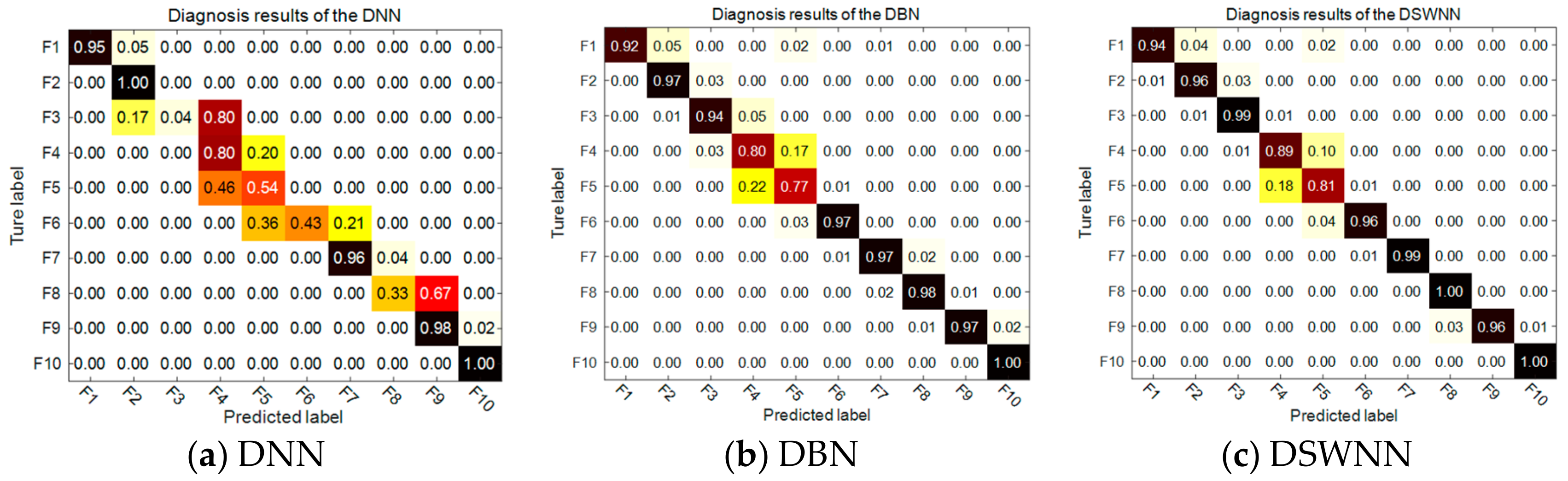
Table 4. It is worth noting that all the data fragments provided are labeled on the basis of the corresponding fault types. During the model training, the DSWNN and DBN were first pre-trained by the data fragments with labels removed, and then they were fine-tuned with these labeled data fragments. Simply, the DNN model used all labeled data for training and validating, which were conducted in a supervised environment.
Figure 8 gives the classification accuracy of the three models. By comparison with the misclassified conditions shown in the confusion matrices, the DNN model easily misjudged the faults of F3, F5, F6, and F8, which was critical as these true negatives could cause serious consequences. F3 and F5 were electrical failures, the occurrence of which has strong randomness and contingency. F6 and F8 were related to the pitch angle, which is supposed to be monitored by wind speed, wind power, pitch encoder, and blade root torque, etc. The reason for these failures is that the random wind speed makes a strong impact on the blades. The essential requirement for diagnosing the above faults is that the classification algorithms used should have the ability to mine implied features from multiple operating data. However, this was exactly what the DNN model lacked because its network parameters were generated by random initialization without any theoretical basis. It is generally known that parameters directly affect the classification results. Fortunately, the DSWNN and DBN models used pre-training to get better network parameters, and their classification accuracy for all failures showed better performance than that of the DNN model (see
Figure 8b,c). But the accuracy in diagnosing the fault F4 and F5 also decreased, which may have been caused by the lack of fault data in the training data.
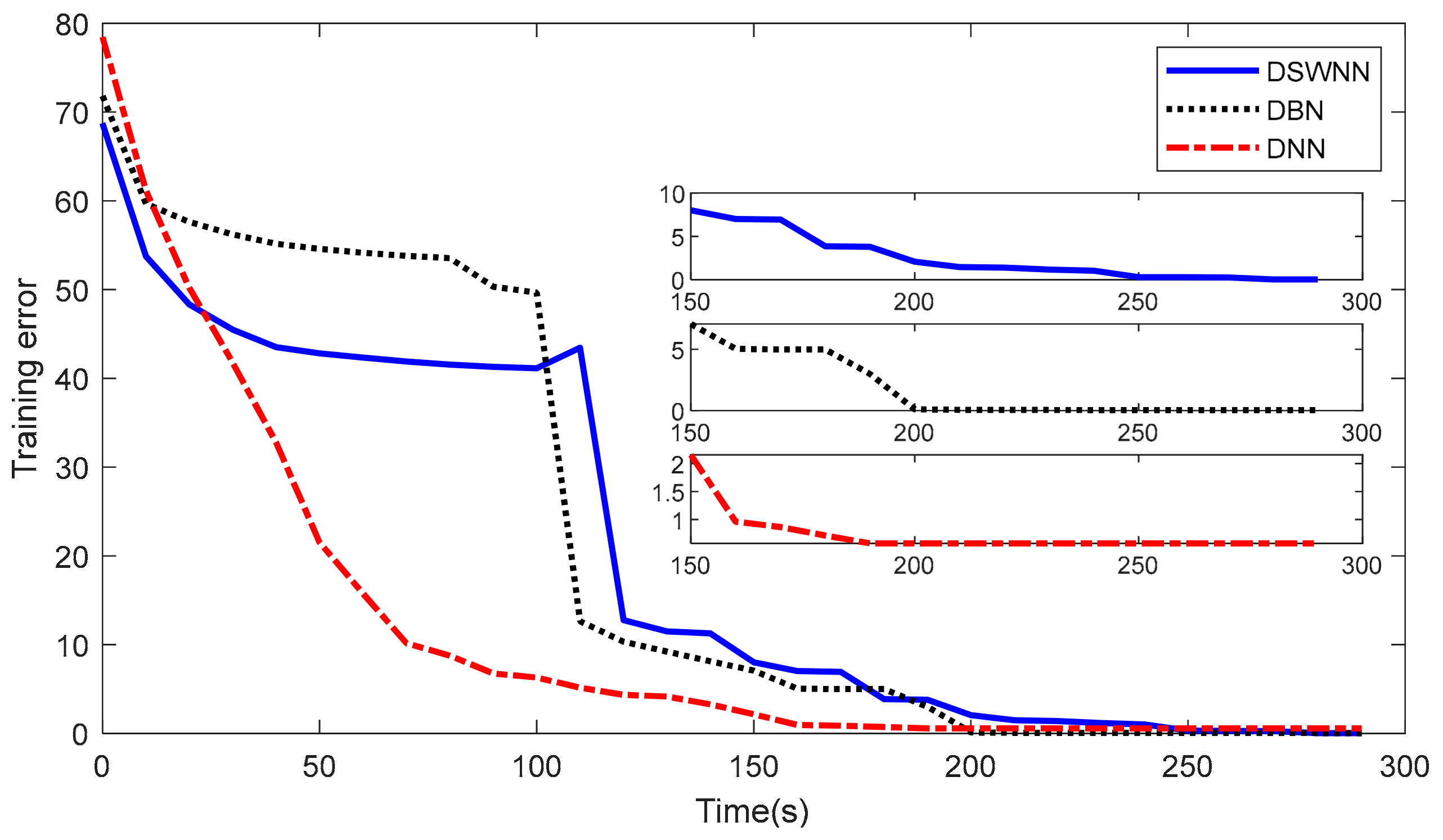
In addition, we also recorded the global changing errors of the three models in the training process at the same time, as shown in
Figure 9. It can be seen from the figure that the convergence times of DSWNN, DBN and DNN were 255 s, 210 s, and 168 s, respectively. DSWNN took the longest time to calculate because it had the small-world transformation process between pre-training and fine-tuning. In a 0–110 s interval, the training errors of DSWNN and DBN almost reached the stage stability, which was because the network was in the pre-training stage and their multiple RBMs had reached the energy conservation. In the range of 110–130 s, DSWNN and DBN changed from unsupervised training to supervised training, and the training error suddenly decreased until a new lower convergence value appeared. Note that at 124 s, the training error of DSWNN increased in a short time, which was due to the additional weights of the add-edges in the network structure after the small-world transformation. The DSWNN retrained the random new add-edges, leading to the short-term error increase.
Seen from the above case studies, the advantages of the DSWNN model appeared mainly in two aspects: (1) the learning ability of the DSWNN model was better than the DBN method, and it was much better than the traditional DNN method; (2) the DSWNN model had very good sensitivity and accuracy in reflecting the condition changes of the wind turbine pitch system; (3) although the DSWNN model was not dominant in time cost, it had a stronger ability to mine deeper feature information from the same data source.


