Dynamic Analysis of Spatial Truss Structures Including Sliding Joint Based on the Geometrically Exact Beam Theory and Isogeometric Analysis

Abstract

With increasing of the size of spatial truss structures, the beam component will be subjected to the overall motion with large deformation. Based on the local frame approach and the geometrically exact beam theory, a beam finite element, which can effectively reduce the rotational nonlinearity and is appropriate for finite motion and deformation issues, is developed. Dynamic equations are derived in the Lie group framework. To obtain the symmetric Jacobian matrix of internal forces, the linearization operation is conducted based on the previously converged configuration. The iteration matrix corresponding to the rotational parameters, including the Jacobian matrix of inertial and internal forces in the initial configuration, can be maintained in the simulation, which drastically improves the computational efficiency. Based on the Lagrangian multiplier method, the constraint equation and its Jacobian matrix of sliding joint are derived. Furthermore, the isogeometric analysis (IGA) based on the non-uniform rational B-splines (NURBS) basis functions, is adopted to interpolate the displacement and rotation fields separately. Finally, three dynamic numerical examples including a deployment dynamic analysis of spatial truss structure are conducted to verify the availability and the applicability of the proposed formulation.

1. Introduction

The deployable spatial truss structure is a typical flexible multibody system consisting of beam members. With the increase of the size, the deployable spatial truss structure usually undergoes finite deformation when refer to finite displacement and rotation. The most common modeling methods in flexible multibody system for beams are the Absolute Nodal Coordinate Formulation (ANCF) and the Geometrically Exact Beam Theory (GEBT). Both approaches can provide the solution of finite deformation and finite motion. The ANCF, proposed by Shabana [1,2], is one of the methods aimed at multibody system dynamics areas recent years. The method uses slopes instead of infinitesimal rotations to simplify the parameter updating algorithm, but at the cost of introducing more degrees of freedom, which reduces the computational efficiency. Comparisons of ANCF and GEBT have been accomplished by Romero [3] and Bauchau et al. [4]. To reduce the computational cost, the latter is employed in this work.

The geometrically exact beam theory (GEBT) is also known as the Simo–Reissner beam theory, which was initially proposed by Reissner [5,6] and then developed by Simo [7,8,9] and other pioneers; for example, Cardona and Géradin [10], Ibrahimbegović et al. [11], and Crisfield and Jelenic [12,13]. In GEBT, the compositions of translations and rotations are typically uncoupled in the space of ${ℝ}^3\times SO(3)$. The cross-section position is considered in the linear space ${ℝ}^3$, while the rotation belongs to a nonlinear space, the special orthogonal group SO(3). In general, the incremental position and rotation variables are described in the global frame, thereby leading to a strong rotational nonlinearity. Based on the classical GEBT, describing the finite rotation variables in the local frame can reduce the rigid rotational nonlinearity. It is implied that the iteration matrix corresponding to the rotation parameters in the initial configuration can be maintained in the simulation, which drastically improves the computational efficiency, especially for the multibody systems, which undergo large displacement and rotation. For cases of finite strain and material nonlinearity, the extension of GEBT can be found in [14,15] based on the Geometric Continuum Mechanics.

An obvious feature of a multibody system is that the connection between different bodies is usually achieved through some joint constraints, such as spherical joint, sliding joint, etc. More different types of classical joint constraints can be found in [16]. For a majority of spatial deployable structures, the sliding joint is often applied and plays an important role. The most common method in defining the friction-free sliding is the Lagrangian multiplier method. Employing this method, Bauchau and Bottasso [17,18] formulated the sliding joint based on the GEBT and pointed out the difference between the prismatic joint and sliding joint, while Sugiyama et al. [19] and Gerstmayr and Shabana [20] modeled the sliding joint applying ANCF. However, the Jacobian matrix of the sliding joint constraint equation is not found in [17,18]. More application of the Lagrangian multiplier on the problems can be found in [21,22]. Besides, there are different methods being employed in modeling sliding joint, such as the master–slave method [23].

Moreover, the Lagrange basis functions have always been applied for finite element discretization in such research, which gives rise to the gap between computer-aided design (CAD) and computer-aided engineering (CAE). The isogeometric analysis (IGA), which was introduced in 2005 by Hughes et al. [24], is filling the traditional gap between CAD and finite element solvers. Over the last decade, IGA has become a well-established method used in structural modeling [25,26,27]. The application of the non-uniform rational B-splines (NURBS) basis functions is shown to be much more advantageous than conventional finite element analysis [28,29]. It is remarked that for the case of sliding along very flexible beam, the IGA method takes more advantage on accuracy and efficiency when using the C^k–continuous NURBS basic function (k ≥ 1). However, under the concept of IGA, the dynamic analysis of the beam structure with a sliding joint, based on the GEBT and Lagrangian multiplier method, has rarely been reported.

The objective of this paper is to propose a geometrically exact beam element based on the local frame approach under the concept of IGA. The proposed element can be applied to the cases of finite deformation and rotation in dynamic analyses of flexible multibody systems, especially for the deployable spatial truss structures with a sliding joint. The analytical expressions of internal and inertial forces and their Jacobian matrices for present beam element are strictly derived based on the framework of Lie group. To obtain a symmetric tangent stiffness, the increments are described based on the previously converged configuration, as suggested by Cardona and Géradin [10]. To promote the integration of CAD and CAE, the displacement and rotation fields are interpolated separately using the NURBS basis functions. Due to the application of the Crisfield and Jelenić interpolation algorithm [12], the strain measures automatically satisfy the property of objectivity. Besides, the dynamic equations expressed in a set of Differential Algebraic Equations (DAEs) are solved by the generalized-α method [30,31]. The sliding joint is modeled using the Lagrangian multiplier method. The constraints equations relative to the sliding joint and its Jacobian matrix are also given.

The paper is organized as follows: The basic theory of the geometrically exact beam theory including beam kinematics, static equations, dynamic equations, and their linearization are introduced in Section 2. Finite element strategies are employed in Section 3. In Section 4, the modeling of sliding joint is conducted. In Section 5, two dynamic numerical examples and a deployment dynamic analysis of spatial truss structure are implemented to verify the availability and the applicability of the formulation proposed in this paper. Conclusions are presented in Section 6.

2. The Geometrically Exact Beam Model

2.1. Beam Kinematics

In this section, a straight beam element with a square cross section was used as an example, and this method can be easily extended to curved beam elements with arbitrary cross sections. A reference configuration ${ℬ}_0$ and a current configuration $ℬ$ are displayed in Figure 1. For an arbitrary cross-section, the reference point of the local frame is assumed to coincide with the centroid $O(o_2,o_3)$. A unit orthogonal basis system $\mathbf{A}=\{{\mathbf{A}}_1,{\mathbf{A}}_2,{\mathbf{A}}_3\}$ along with the material coordinates $\{{\xi }_1,{\xi }_2,{\xi }_3\}$ is introduced. The axis of the beam is initially along ${\mathbf{A}}_1$, with the length of beam l and the arc-length parameter $S={\xi }_1\in \left[0,l\right]$ of the spatial curve. The orientation of the cross-section is described by the basis vectors $\{{\mathbf{A}}_2,{\mathbf{A}}_3\}$. The local frame $\mathbf{a}=\{{\mathbf{a}}_1,{\mathbf{a}}_2,{\mathbf{a}}_3\}$ is attached to the cross-section in the current configuration, which is characterized by the time parameter t. For convenience, it is assumed that the material frame ${\mathbf{A}}_i$ and inertial frame ${\mathbf{e}}_i$ initially coincide, and thus the relationship between the basis vectors ${\mathbf{A}}_i$ and ${\mathbf{a}}_i$ is as follows:

$${\mathbf{a}}_i=\mathbf{R}{\mathbf{A}}_i\mathrm{for}i=1,2,3$$

(1)

where the operator R is the cross-section orthogonal rotation tensor with respect to inertial frame. In general, the rotation tensor is defined from the exponential map and can be expressed directly by Rodrigues formula [32]:

$$\mathbf{R}=\exp (\tilde{\mathbf{\Theta }})={\mathbf{I}}_{3\times 3}+a_1(\mathbf{\Theta })\tilde{\mathbf{\Theta }}+a_2(\mathbf{\Theta })\tilde{\mathbf{\Theta }}\tilde{\mathbf{\Theta }}$$

(2)

with

$$a_1(\mathbf{\Theta })=\frac{\sin (\Vert \mathbf{\Theta }\Vert )}{\Vert \mathbf{\Theta }\Vert },a_2(\mathbf{\Theta })=\frac{1-\cos (\Vert \mathbf{\Theta }\Vert )}{{\Vert \mathbf{\Theta }\Vert }^2}$$

(3)

The notation $\widetilde{•}$ indicates that there is an invertible linear map from ${ℝ}^k$ to the Lie algebra; and the expression of which depends on the dimension k. The variable $\tilde{\mathbf{\Theta }}$ in the SO(3) framework represents the skew-symmetric matrix of the rotational vector $\mathbf{\Theta }$ and $\Vert \mathbf{\Theta }\Vert$ means the magnitude of the rotational vector. On the contrary, the inverse map of the exponential map is the logarithmic map [33], giving:

$$\log (\mathbf{R})=\tilde{\mathbf{\Theta }}=\{\begin{array}{cc}{\mathbf{0}}_3& \mathrm{if}\mathbf{R}={\mathbf{I}}_{3\times 3}\\ \frac{\theta }{2\sin \left(\theta \right)}(\mathbf{R}-{\mathbf{R}}^T)& \mathrm{if}\mathbf{R}\ne {\mathbf{I}}_{3\times 3}\end{array}$$

(4)

with $\theta =\arccos \left(\frac{1}{2}(\mathrm{trace}(\mathbf{R})-1)\right)$ and the absolute value $\left|\theta \right|<\pi$.

An arbitrary point p on the cross-section in the current configuration can be expressed by:

$${\mathbf{x}}_p({\xi }_1,{\xi }_2,{\xi }_3)=\mathbf{x}\left({\xi }_1)+\mathbf{R}\right({\xi }_1){\mathbf{y}}_p({\xi }_2,{\xi }_3)$$

(5)

in which ${\mathbf{y}}_p={\xi }_2{\mathbf{A}}_2+{\xi }_3{\mathbf{A}}_3$, and is defined from the reference configuration since the cross-section is assumed to remain undeformed.

2.2. Beam Statics and Its Linearization

According to continuum mechanics, the Green-Lagrangian strain tensor $\mathbf{E}({\xi }_1,{\xi }_2,{\xi }_3)$ is defined as:

$$E_{ij}=\frac{1}{2}\left(F_{ik}^{\mathrm{T}}{F}_{kj}-{\delta }_{ij}\right)=\frac{1}{2}\left(\frac{\partial {\mathbf{x}}_p^{\mathrm{T}}}{\partial {\xi }_i}\frac{\partial {\mathbf{x}}_p}{\partial {\xi }_j}-\frac{\partial {\mathbf{x}}_p^{0\mathrm{T}}}{\partial {\xi }_i}\frac{\partial {\mathbf{x}}_p^0}{\partial {\xi }_j}\right)$$

(6)

in which $F_{kj}$ is the deformation gradient, and ${\delta }_{ij}$ is the Kronecker delta. The derivatives of the displacement field in Equation (5) with respect to ${\xi }_i(i=1,2,3)$ are given by:

$$\{\begin{array}{l}\frac{\partial {\mathbf{x}}_p({\xi }_1,{\xi }_2,{\xi }_3)}{\partial {\xi }_1}={\mathbf{x}}^{\mathbf{\prime }}+{\mathbf{R}}^{\mathbf{\prime }}{\mathbf{y}}_p\\ \frac{\partial {\mathbf{x}}_p({\xi }_1,{\xi }_2,{\xi }_3)}{\partial {\xi }_2}=\mathbf{R}{\mathbf{A}}_2\\ \frac{\partial {\mathbf{x}}_p({\xi }_1,{\xi }_2,{\xi }_3)}{\partial {\xi }_3}=\mathbf{R}{\mathbf{A}}_3\end{array}$$

(7)

where $(\cdot {)}^{\prime }$ denotes the derivative relative to arc-length parameter S.

In the classical geometrically exact beam theory, the strain measures $\mathsf{\epsilon }$ can be represented as:

$$\mathsf{\epsilon }=\left[\begin{array}{c}\mathsf{\gamma }\\ \mathsf{\kappa }\end{array}\right]=\left[\begin{array}{c}{\mathbf{R}}^{\mathrm{T}}{\mathbf{x}}^{\mathbf{\prime }}-{\mathbf{R}}^{\mathrm{T}}{{\mathbf{x}}^{\mathbf{\prime }}}_0\\ \mathbf{T}{\mathbf{\Theta }}^{\mathbf{\prime }}-\mathbf{T}{{\mathbf{\Theta }}^{\mathbf{\prime }}}_0\end{array}\right]$$

(8)

For an initially straight beam, the strain measures $\mathsf{\epsilon }$ can be thus written as:

$$\mathsf{\epsilon }=\left[\begin{array}{c}\mathsf{\gamma }\\ \mathsf{\kappa }\end{array}\right]=\left[\begin{array}{c}{\mathbf{R}}^{\mathrm{T}}{\mathbf{x}}^{\mathbf{\prime }}-{\mathbf{A}}_1\\ \mathbf{T}{\mathbf{\Theta }}^{\mathbf{\prime }}\end{array}\right]$$

(9)

in which $\mathsf{\gamma }={[{\gamma }_1,{\gamma }_2,{\gamma }_3]}^{\mathrm{T}}$ quantifies the beam axis extension and two shearing; $\mathsf{\kappa }={[{\kappa }_1,{\kappa }_2,{\kappa }_3]}^{\mathrm{T}}$ measures its twist and two curvatures in local frame. The tangent operator can be obtained from [10], giving:

$$\mathbf{T}={\mathbf{I}}_{3\times 3}-a_2(\mathbf{\Theta })\tilde{\mathbf{\Theta }}+a_3(\mathbf{\Theta })\tilde{\mathbf{\Theta }}\tilde{\mathbf{\Theta }}$$

(10)

with the coefficients:

$$a_3(\mathbf{\Theta })=\frac{\Vert \mathbf{\Theta }\Vert -\sin (\Vert \mathbf{\Theta }\Vert )}{{\Vert \mathbf{\Theta }\Vert }^3}{a}_4(\mathbf{\Theta })=\frac{1}{{\Vert \mathbf{\Theta }\Vert }^2}\left(1-\frac{\Vert \mathbf{\Theta }\Vert }{2}\cot (\frac{\Vert \mathbf{\Theta }\Vert }{2})\right)$$

(11)

Consequently, based on the rigid perimeter and small strain assumptions, the non-vanishing terms in Equation (6) can be given as:

$$\mathbf{E}=\left[\begin{array}{ccc}{\gamma }_1+{\kappa }_3{\xi }_2-{\kappa }_2{\xi }_3& \frac{1}{2}({\gamma }_2+{\kappa }_1{\xi }_3)& \frac{1}{2}({\gamma }_3-{\kappa }_1{\xi }_2)\\ \frac{1}{2}({\gamma }_2+{\kappa }_1{\xi }_3)& 0& 0\\ \frac{1}{2}({\gamma }_3-{\kappa }_1{\xi }_2)& 0& 0\end{array}\right]$$

(12)

Assuming a constitutive law of isotropic linear elastic materials, the second Piola–Kirchhoff stress tensor $\mathbf{S}={[{\mathrm{S}}_{11},{\mathrm{S}}_{12},{\mathrm{S}}_{13}]}^{\mathrm{T}}$ refers to:

$$\mathbf{S}=\mathbf{DE},\mathbf{D}=\left[\begin{array}{ccc}E& 0& 0\\ 0& G& 0\\ 0& 0& G\end{array}\right]$$

(13)

in which E, and G are the elasticity modulus and shear modulus, respectively. Based on the Green-Lagrange strain tensor, the internal virtual work can be computed as:

$$\mathsf{\delta }{\mathcal{W}}_{\mathrm{int}}={\displaystyle {\int }_V\mathsf{\delta }{\mathbf{E}}^{\mathrm{T}}\mathbf{S}\mathrm{d}V}={\displaystyle {\int }_l\mathsf{\delta }{\overline{\mathbf{E}}}^{\mathrm{T}}\overline{\mathbf{D}}\overline{\mathbf{E}}\mathrm{d}{\xi }_1}$$

(14)

with $\overline{\mathbf{E}}=\mathsf{\epsilon }$ and the elastic matrix:

$$\overline{\mathbf{D}}=\left[\begin{array}{cccccc}EA& 0& 0& 0& 0& 0\\ & \tau GA& 0& 0& 0& 0\\ & & \tau GA& 0& 0& 0\\ & & & G{I}_0& 0& 0\\ & & \mathrm{Sym}& & E{I}_{33}& -E{I}_{32}\\ & & & & & E{I}_{22}\end{array}\right]$$

(15)

where $\tau$ is the shear coefficient. The notation A in Equation (15) denotes the area of the cross-section and four constant section properties are calculated from the following formulas:

$$I_{22}={\displaystyle {\int }_A{\xi }_2^2\mathrm{d}A},I_{33}={\displaystyle {\int }_A{\xi }_3^2\mathrm{d}A,}{I}_{32}={\displaystyle {\int }_A{\xi }_2{\xi }_3\mathrm{d}A},I_0=I_{22}+I_{33}$$

(16)

The stress measures can be given by:

$$\overline{\mathbf{S}}=\overline{\mathbf{D}}\overline{\mathbf{E}}={\left[\begin{array}{cc}{\mathbf{N}}^{\mathrm{T}}& {\mathbf{M}}^{\mathrm{T}}\end{array}\right]}^{\mathrm{T}}$$

(17)

in which the stress resultant $\mathbf{N}={[{\mathrm{N}}_1,{\mathrm{N}}_2,{\mathrm{N}}_3]}^{\mathrm{T}}$ represents one normal force and two shear forces in local frame; the stress couple $\mathbf{M}={[{\mathrm{M}}_1,{\mathrm{M}}_2,{\mathrm{M}}_3]}^{\mathrm{T}}$ includes one torsional moment and two bending moments in local frame.

According to Equation (9) the variation of the strain measures can be written as:

$$\mathsf{\delta }\overline{\mathbf{E}}=\mathsf{\delta }\mathsf{\epsilon }=\left[\begin{array}{c}\mathsf{\delta }\mathsf{\gamma }\\ \mathsf{\delta }\mathsf{\kappa }\end{array}\right]=\mathbf{B}\mathsf{\delta }\mathbf{h}$$

(18)

with $\mathsf{\delta }\mathbf{h}={[\mathsf{\delta }{\mathbf{x}}^{\mathrm{T}},\mathsf{\delta }{\mathbf{\Theta }}^{\mathrm{T}}]}^{\mathrm{T}}$ and the strain operator:

$$\mathbf{B}=\left[\begin{array}{cc}{\mathbf{R}}^{\mathrm{T}}\frac{\partial }{\partial {\xi }_1}& \widetilde{{\mathbf{R}}^{\mathrm{T}}{\mathbf{x}}^{\mathbf{\prime }}}\\ 0& \frac{\partial }{\partial {\xi }_1}+\tilde{\mathsf{\kappa }}\end{array}\right]$$

(19)

In each iterative step, the computed rotation increments lie in the tangent space of the current configuration. To obtain a symmetric tangent stiffness, as suggested by [10], the rotation variation in local frame is transformed in terms of the rotation increment $\mathsf{\phi }$ with respect to previously converged configuration with the relationship:

$$\mathsf{\delta }\mathbf{\Theta }=\mathbf{T}\mathsf{\delta }\mathsf{\phi }$$

(20)

Then the Equation (18) can be further expressed as:

$$\mathsf{\delta }\overline{\mathbf{E}}={\mathbf{B}}^{\ast }\mathsf{\delta }{\mathbf{h}}^{\ast }$$

(21)

with the generalized displacement variations $\mathsf{\delta }{\mathbf{h}}^{\ast }={[\mathsf{\delta }{\mathbf{x}}^{\mathrm{T}},\mathsf{\delta }{\mathsf{\phi }}^{\mathrm{T}}]}^{\mathrm{T}}$ and the strain operator:

$${\mathbf{B}}^{*}=\left[\begin{array}{cc}{\mathbf{R}}^{\mathrm{T}}\frac{\partial }{\partial {\xi }_1}& (\widetilde{{\mathbf{R}}^{\mathrm{T}}{\mathbf{x}}^{\mathbf{\prime }}})\mathbf{T}\\ 0& \mathbf{T}\frac{\partial }{\partial {\xi }_1}+{\mathbf{T}}^{\mathbf{\prime }}+\tilde{\mathsf{\kappa }}\mathbf{T}\end{array}\right]$$

(22)

Then the internal virtual work can be further written as:

$$\mathsf{\delta }{\mathcal{W}}_{\mathrm{int}}={\displaystyle {\int }_l\mathsf{\delta }{\mathbf{h}}^{\ast \mathrm{T}}{\mathbf{B}}^{\ast \mathrm{T}}\overline{\mathbf{S}}\mathrm{d}{\xi }_1}$$

(23)

Thus, the tangent stiffness matrix can be derived by linearization of Equation (23), giving:

$$\Delta \left(\mathsf{\delta }{\mathcal{W}}_{\mathrm{int}}\right)={\displaystyle {\int }_l\mathsf{\delta }{\mathbf{h}}^{\ast \mathrm{T}}{\mathbf{B}}^{\ast \mathrm{T}}\overline{\mathbf{D}}{\mathbf{B}}^{\ast }\Delta {\mathbf{h}}^{\ast }+\mathsf{\delta }{\mathbf{h}}^{\ast \mathrm{T}}\Delta {\mathbf{B}}^{\ast \mathrm{T}}\left[\begin{array}{c}\mathbf{N}\\ \mathbf{M}\end{array}\right]\mathrm{d}{\xi }_1}={\displaystyle {\int }_l\mathsf{\delta }{\mathbf{h}}^{\ast \mathrm{T}}\mathbf{\Pi }\Delta {\mathbf{h}}^{\ast }+\mathsf{\delta }{\mathbf{h}}^{\ast \mathrm{T}}\mathsf{\Upsilon }\Delta {\mathbf{h}}^{\ast }\mathrm{d}{\xi }_1}$$

(24)

in which the first term is the material part and the second term is the geometric part. By introducing an operator $\mathbf{\Xi }$, the continuous geometric stiffness matrix can be further obtained, giving:

$$\mathsf{\Upsilon }=\left[\begin{array}{cc}\mathbf{0}& -{\left(\frac{\partial }{\partial {\xi }_1}\right)}^{\mathrm{T}}\mathbf{R}\tilde{\mathbf{N}}\mathbf{T}\\ {\mathbf{T}}^{\mathrm{T}}\tilde{\mathbf{N}}{\mathbf{R}}^{\mathrm{T}}\left(\frac{\partial }{\partial {\xi }_1}\right)& \begin{array}{l}{\mathbf{T}}^{\mathrm{T}}\tilde{\mathbf{N}}(\widetilde{{\mathbf{R}}^{\mathrm{T}}{\mathbf{x}}^{\mathbf{\prime }}})\mathbf{T}+{\mathbf{T}}^{\mathrm{T}}\tilde{\mathbf{M}}\tilde{\mathsf{\kappa }}\mathbf{T}+{\mathbf{T}}^{\mathrm{T}}\tilde{\mathbf{M}}{\mathbf{T}}^{\mathbf{\prime }}+\mathbf{H}+\mathbf{\Xi }(\Delta {\mathbf{T}}^{\mathrm{T}}\tilde{\mathbf{N}}{\mathbf{R}}^{\mathrm{T}}{\mathbf{x}}^{\mathbf{\prime }})\\ +\mathbf{\Xi }(\Delta {\mathbf{T}}^{\mathrm{T}}\tilde{\mathbf{M}}\mathsf{\kappa })+{\left(\frac{\partial }{\partial {\xi }_1}\right)}^{\mathrm{T}}\mathbf{\Xi }(\Delta {\mathbf{T}}^{\mathrm{T}}\mathbf{M})+\left(\mathbf{\Xi }(\Delta {\mathbf{T}}^{\mathrm{T}}\mathbf{M})+{\mathbf{T}}^{\mathrm{T}}\tilde{\mathbf{M}}\mathbf{T}\right)\left(\frac{\partial }{\partial {\xi }_1}\right)\end{array}\end{array}\right]$$

(25)

where H is computed by the formula:

$$\begin{array}{ll}\mathbf{H}& =c_1\mathbf{M}\otimes {\mathbf{\Theta }}^{\mathbf{\prime }}+c_2[(\tilde{\mathbf{\Theta }}\mathbf{M})\otimes {\mathbf{\Theta }}^{\mathbf{\prime }}-({{\mathbf{\Theta }}^{\mathbf{\prime }}}^{\mathrm{T}}\mathbf{\Theta })\tilde{\mathbf{M}}+(\widetilde{{\mathbf{\Theta }}^{\mathbf{\prime }}}\mathbf{M})\otimes \mathbf{\Theta }]+c_3[({\mathbf{M}}^{\mathrm{T}}\mathbf{\Theta }){\mathbf{\Theta }}^{\mathbf{\prime }}\otimes \mathbf{\Theta }+({\mathbf{M}}^{\mathrm{T}}{\mathbf{\Theta }}^{\mathbf{\prime }})\mathbf{\Theta }\otimes \mathbf{\Theta }]\\ & +c_3[({\mathbf{M}}^{\mathrm{T}}\mathbf{\Theta })\mathbf{\Theta }\otimes {\mathbf{\Theta }}^{\mathbf{\prime }}+({{\mathbf{\Theta }}^{\mathbf{\prime }}}^{\mathrm{T}}\mathbf{\Theta }){\mathbf{M}}^{\mathrm{T}}\mathbf{\Theta }{\mathsf{{\rm I}}}_3+({{\mathbf{\Theta }}^{\mathbf{\prime }}}^{\mathrm{T}}\mathbf{\Theta })\mathbf{\Theta }\otimes \mathbf{M}]+c_5({\mathbf{\Theta }}^{\mathbf{\prime }}\otimes \mathbf{M}+{\mathbf{\Theta }}^{\mathbf{\prime }}\mathbf{M}{\mathsf{{\rm I}}}_3)\\ & +b_1({{\mathbf{\Theta }}^{\mathbf{\prime }}}^{\mathrm{T}}\mathbf{\Theta })\mathbf{M}\otimes \mathbf{\Theta }+b_2({{\mathbf{\Theta }}^{\mathbf{\prime }}}^{\mathrm{T}}\mathbf{\Theta })(\tilde{\mathbf{\Theta }}\mathbf{M})\otimes \mathbf{\Theta }+b_3({{\mathbf{\Theta }}^{\mathbf{\prime }}}^{\mathrm{T}}\mathbf{\Theta })({\mathbf{M}}^{\mathrm{T}}\mathbf{\Theta })\mathbf{\Theta }\otimes \mathbf{\Theta }\end{array}$$

(26)

with the coefficients,

$$\begin{array}{l}{c}_1=\frac{\Vert \mathbf{\Theta }\Vert \cos \Vert \mathbf{\Theta }\Vert -\sin \Vert \mathbf{\Theta }\Vert }{{\Vert \mathbf{\Theta }\Vert }^3},c_2=\frac{\Vert \mathbf{\Theta }\Vert \sin \Vert \mathbf{\Theta }\Vert +2\cos \Vert \mathbf{\Theta }\Vert -2}{{\Vert \mathbf{\Theta }\Vert }^4},c_3=\frac{3\sin \Vert \mathbf{\Theta }\Vert -2\Vert \mathbf{\Theta }\Vert -\Vert \mathbf{\Theta }\Vert \cos \Vert \mathbf{\Theta }\Vert }{{\Vert \mathbf{\Theta }\Vert }^5},\\ c_4=\frac{1-\cos \Vert \mathbf{\Theta }\Vert }{{\Vert \mathbf{\Theta }\Vert }^2},c_5=\frac{\Vert \mathbf{\Theta }\Vert -\sin \Vert \mathbf{\Theta }\Vert }{{\Vert \mathbf{\Theta }\Vert }^3},b_1=\frac{(3-{\Vert \mathbf{\Theta }\Vert }^2)\sin \Vert \mathbf{\Theta }\Vert -3\Vert \mathbf{\Theta }\Vert \cos \Vert \mathbf{\Theta }\Vert }{{\Vert \mathbf{\Theta }\Vert }^5},\\ b_2=\frac{({\Vert \mathbf{\Theta }\Vert }^2-8)\cos \Vert \mathbf{\Theta }\Vert -5\Vert \mathbf{\Theta }\Vert \sin \Vert \mathbf{\Theta }\Vert +8}{{\Vert \mathbf{\Theta }\Vert }^6},b_3=\frac{({\Vert \mathbf{\Theta }\Vert }^2-15)\sin \Vert \mathbf{\Theta }\Vert +7\Vert \mathbf{\Theta }\Vert \cos \Vert \mathbf{\Theta }\Vert +8\Vert \mathbf{\Theta }\Vert }{{\Vert \mathbf{\Theta }\Vert }^7}.\end{array}$$

(27)

For arbitrary 3 × 1 vector u, the operator $\mathbf{\Xi }$ can be expressed as:

$$\mathbf{\Xi }(\Delta {\mathbf{T}}^{\mathrm{T}}\mathbf{u})=c_1(\mathbf{u}\otimes \mathbf{\Theta })+c_2[(\tilde{\mathbf{\Theta }}\mathbf{u})\otimes \mathbf{\Theta }]+c_3[({\mathbf{\Theta }}^{\mathrm{T}}\mathbf{u})\mathbf{\Theta }\otimes \mathbf{\Theta }]-c_4\tilde{\mathbf{u}}+c_5[({\mathbf{\Theta }}^{\mathrm{T}}\mathbf{u}){\mathbf{I}}_3+\mathbf{\Theta }\otimes \mathbf{u}]$$

(28)

The matrices $\mathbf{\Pi }$ in the material part are symmetric. The $\mathsf{\Upsilon }$ in the geometric part obtained here shows non-obvious symmetry in its formula structure, although it is numerically symmetric. In the case of small deformation, the geometric stiffness is unnecessary in general. However, numerical examples show that the application of geometric stiffness can improve the convergence of Newton iterations for cases of both small deformation and finite deformation.

2.3. Beam Dynamics and Its Linearization

The weak form of dynamic equilibrium equation can be expressed as:

$$\mathsf{\delta }{\mathcal{W}}_{\mathrm{int}}-\mathsf{\delta }{\mathcal{W}}_{\mathrm{ext}}+\mathsf{\delta }{\mathcal{W}}_{\mathrm{ine}}=0$$

(29)

with the internal virtual work $\mathsf{\delta }{\mathcal{W}}_{\mathrm{int}}$, external virtual work $\mathsf{\delta }{\mathcal{W}}_{\mathrm{ext}}$, and inertial virtual work $\mathsf{\delta }{\mathcal{W}}_{\mathrm{ine}}$. Denoting ρ as the mass density of the material, the inertial virtual work $\mathsf{\delta }{\mathcal{W}}_{\mathrm{ine}}$ is given by:

$$\mathsf{\delta }{\mathcal{W}}_{\mathrm{ine}}={\displaystyle \iint \rho \mathsf{\delta }{\mathbf{x}}_p^{\mathrm{T}}{\ddot{\mathbf{x}}}_p}dAd{\xi }_1=A_{\rho }{\displaystyle {\int }_l\mathsf{\delta }{\mathbf{h}}^{\mathrm{T}}\left[\begin{array}{c}\ddot{\mathbf{x}}\\ \mathbf{J}\mathsf{\alpha }+\tilde{\mathbf{\Omega }}(\mathbf{J}\mathbf{\Omega })\end{array}\right]}\mathrm{d}{\xi }_1$$

(30)

where $A_{\rho }=A\rho$ is the density of the cross-section. $\mathsf{\alpha }$ and Ω are the angular acceleration and angular velocity of beam cross-section in local frame, respectively. Besides, the notation $\mathbf{J}$ denotes the cross-sectional moment of inertia with relative to the centroid, giving:

$$\mathbf{J}=\left[\begin{array}{ccc}{I}_0& 0& 0\\ 0& I_{33}& -I_{23}\\ 0& -I_{23}& I_{22}\end{array}\right]$$

(31)

Then the generalized mass matrix can be derived by linearization of the inertial virtual work $\mathsf{\delta }{\mathcal{W}}_{\mathrm{ine}}$, giving:

$$\Delta (\mathsf{\delta }{\mathcal{W}}_{\mathrm{ine}})=A_{\rho }{\displaystyle {\int }_l\mathsf{\delta }{\mathbf{h}}^{\ast \mathrm{T}}\left[\begin{array}{cc}{\mathbf{I}}_3\left(\frac{{\mathrm{d}}^2}{\mathrm{d}{t}^2}\right)& {\mathbf{0}}_3\\ {\mathbf{0}}_3& {\mathbf{T}}^{\mathrm{T}}\left[\begin{array}{l}\left(\mathbf{J}\tilde{\mathsf{\alpha }}-\widetilde{(\mathbf{J}\mathbf{\Omega })}\tilde{\mathbf{\Omega }}+\tilde{\mathbf{\Omega }}\mathbf{J}\tilde{\mathbf{\Omega }}\right)+\\ \left(\mathbf{J}\tilde{\mathbf{\Omega }}-\widetilde{(\mathbf{J}\mathbf{\Omega })}+\tilde{\mathbf{\Omega }}\mathbf{J}\right)\left(\frac{\mathrm{d}}{\mathrm{d}t}\right)+\mathbf{J}\left(\frac{{\mathrm{d}}^2}{\mathrm{d}{t}^2}\right)\end{array}\right]\mathbf{T}\end{array}\right]\Delta {\mathbf{h}}^{\ast }\mathrm{d}{\xi }_1}$$

(32)

Since the virtual rotational vector $\mathsf{\delta }\mathsf{\phi }$ is defined in the local frame, it is free from the influence of rigid rotation, which greatly reduces the rotational nonlinearity. Consequently, the parts of the stiffness matrix and the generalized mass matrix, which corresponds to the rotation parameters, are invariable under arbitrary rigid motion. Thereby, the number of updates required during the computation process decreases sharply.

Similarly, the external virtual work can be computed by:

$$\mathsf{\delta }{\mathcal{W}}_{\mathrm{ext}}={\displaystyle \int \left[\mathsf{\delta }{\mathbf{x}}^{\mathrm{T}}\mathbf{F}+\mathsf{\delta }{\mathsf{\phi }}^{\mathrm{T}}{\mathbf{T}}^{\mathrm{T}}\mathbf{P}\right]\mathrm{d}{\xi }_1}+\mathsf{\delta }\mathbf{x}{(\xi )}^{\mathrm{T}}\overline{\mathbf{F}}+\mathsf{\delta }\mathsf{\phi }{(\xi )}^{\mathrm{T}}{\mathbf{T}}^{\mathrm{T}}\overline{\mathbf{P}}$$

(33)

where F and $\overline{\mathbf{F}}$ represent the distributed force and the concentrated force on the centerline of the beam in the inertial frame, respectively. P and $\overline{\mathbf{P}}$ represent the distributed moment and the concentrated moment on the cross-section of the beam in the local frame, respectively.

3. Finite Element Formulation

3.1. Spatial Discretization: NURBS Basis Functions

In general, the dynamics equilibrium equations of the geometrically exact beam can be transformed into a set of nonlinear algebraic equations by finite element spatial discretization and time discretization. In the spatial domain, the linearized governing equations described above are discretized by adopting the IGA; namely, both the geometry and the unknown variables are approximated by NURBS [24].

Denote Ψ as a non-decreasing knot vector, giving:

$$\mathbf{\Psi }=\left\{{\Psi }_1,\cdots ,{\Psi }_{n+\varsigma +1}\right\}$$

(34)

with the degree of basis functions ϛ and the number of control point n. According to the Cox-de Boor recursion formula, a B-spline basis function can be obtained from a linear combination of two B-spline basis functions of degree ϛ-1, giving:

$${\chi }_{i,\varsigma }\left(\Psi \right)=\frac{\Psi -{\Psi }_i}{{\Psi }_{i+\varsigma }-{\Psi }_i}{\chi }_{i,\varsigma -1}\left(\Psi \right)+\frac{{\Psi }_{i+\varsigma +1}-\Psi }{{\Psi }_{i+\varsigma +1}-{\Psi }_{i+1}}{\chi }_{i+1,\varsigma -1}\left(\Psi \right)$$

(35)

with

$${\chi }_{i,0}\left(\Psi \right)=\{\begin{array}{l}1\mathrm{if}{\Psi }_i\le \Psi <{\Psi }_{i+1}\hfill \\ 0otherwise\hfill \end{array}$$

(36)

when ϛ = 0.

Then, a NURBS basis function can be derived through introducing the weight factors $w_i$, giving:

$$N_{i,\varsigma }\left(\Psi \right)=\frac{{\chi }_{i,\varsigma }\left(\Psi \right)w_i}{{\displaystyle {\sum }_{j=1}^m{\chi }_{j,\varsigma }\left(\Psi \right)w_j}}$$

(37)

in which ${\chi }_{i,\varsigma }$ is the B-spline basis function. Obviously, the NURBS basis function degenerates into the B-spline basis function when all weight factors are equal to one. The position coordinate vector of any point can be calculated from interpolation and written as:

$$\mathbf{r}\left(\Psi \right)={\displaystyle \sum _{i=1}^m{N}_{i,\varsigma }{\mathbb{P}}_i}$$

(38)

where ${\mathbb{P}}_i$ is the control point.

The continuity of the NURBS basis function is determined by the multiplicity of a knot. Given multiplicity k of a knot, the continuity of the basis function is $C^{\infty }$ between knots, while it is $C^{\varsigma -k}$ at the knot. Thus, NURBS can accurately describe various types of curves and surfaces, such as circles, hyperbolas, and elliptic surfaces.

3.2. Discretization of the Linearized Equations

It is worth noting that separate interpolations of the displacement and rotation fields are conducted to make the geometric representations uniform in the finite element analysis and CAD. Since the displacement field takes values in linear space ${ℝ}^3$ while the rotation field in nonlinear manifold SO(3), the interpolations of the displacement and rotation field are conducted in different methods. To satisfy the objectivity of strain measures, the Crisfield and Jelenić interpolation algorithm [12] is adopted, in which the relative rotation is interpolated. The interpolation formulas are given by:

$$\mathbf{x}=N_I{\mathbf{x}}_I,{\mathbf{x}}^{\mathbf{\prime }}={N^{\prime }}_I{\mathbf{x}}_I$$

(39)

$${\mathbf{\Theta }}_I^{\mathrm{r}}=N_I\log ({\mathbf{R}}_{\mathrm{r}}^{-1}{\mathbf{R}}_I)$$

(40)

where $N_I$ is the NURBS basis function corresponding to control point I, and a summation is extended to all the control points of the element. The notation ${\mathbf{\Theta }}_I^{\mathrm{r}}$ is the relative rotation, and ${\mathbf{R}}_{\mathrm{r}}$ is the rotation matrix of the reference point, which is typically chosen as the first control point on an element. The strain measures can thus be interpolated as:

$$\mathsf{\epsilon }=\left[\begin{array}{c}\mathsf{\gamma }\\ \mathsf{\kappa }\end{array}\right]=\left[\begin{array}{c}{\mathbf{R}}^{\mathrm{T}}{N^{\prime }}_I{\mathbf{x}}_I-{\mathbf{A}}_1\\ \mathbf{T}(N_I{\mathbf{\Theta }}_I^{\mathrm{r}}){N^{\prime }}_I{\mathbf{\Theta }}_I^{\mathrm{r}}\end{array}\right]$$

(41)

With

$$\mathbf{R}={\mathbf{R}}_{\mathrm{r}}\exp ({\tilde{\mathbf{\Theta }}}^{\mathrm{r}})$$

(42)

Hence, the generalized displacement variation and its derivative can be discretized into:

$$\mathsf{\delta }{\mathbf{h}}^{\ast }=N_I\mathsf{\delta }{\mathbf{h}}_I^{\ast },\mathsf{\delta }{\mathbf{h}}^{\ast }{}^{\prime }={N^{\prime }}_I\mathsf{\delta }{\mathbf{h}}_I^{\ast }$$

(43)

where $\mathsf{\delta }{\mathbf{h}}_I^{\ast }$ is the generalized displacement variation of the control point. The strain-displacements matrix ${\mathbf{B}}_I^{*}$ is the discrete counterpart of the strains operator ${\mathbf{B}}_{}^{*}$, as shown in Equation (22), giving:

$${\mathbf{B}}_I^{*}=\left[\begin{array}{cc}{\mathbf{R}}^{\mathrm{T}}{N^{\prime }}_I& (\widetilde{{\mathbf{R}}^{\mathrm{T}}{\mathbf{x}}^{\mathbf{\prime }}})\mathbf{T}{N}_I\\ 0& \mathbf{T}{N^{\prime }}_I+({\mathbf{T}}^{\mathbf{\prime }}+\tilde{\mathsf{\kappa }}\mathbf{T})N_I\end{array}\right]$$

(44)

Consequently, the strain measures can be written as:

$$\mathsf{\delta }\overline{\mathbf{E}}={\mathbf{B}}_I^{\ast }\mathsf{\delta }{\mathbf{h}}_I^{\ast }$$

(45)

The generalized internal force and inertial force can be discretized from Equations (23) and (30) as:

$${\mathbf{F}}_I^{\mathrm{int}}={\displaystyle {\int }_l{\mathbf{B}}_I^{*\mathrm{T}}\overline{\mathbf{S}}\mathrm{d}{\xi }_1}$$

(46)

$${\mathbf{F}}_I^{\mathrm{ine}}={\displaystyle {\int }_l{A}_{\rho }{N}_I^{\mathrm{T}}\left[\begin{array}{c}\ddot{\mathbf{x}}\\ {\mathbf{T}}^{\mathrm{T}}\mathbf{J}\mathsf{\alpha }+{\mathbf{T}}^{\mathrm{T}}\tilde{\mathbf{\Omega }}(\mathbf{J}\mathbf{\Omega })\end{array}\right]}\mathrm{d}{\xi }_1$$

(47)

In this work, as a separate interpolation is employed, shear locking exists in 1-order elements and is circumvented by the selective reduced integration. The one-point quadrature strategy is employed to calculate the shear strain, while the full quadrature, i.e., two-point quadrature for 1-order element is used to calculate the membrane and bending strains. Besides, high-order elements will not suffer from the shear locking problem and the full quadrature is employed to obtain all the strains in the Equations (46) and (47).

3.3. Time Discretization: Lie Group Generalized-α Method

The dynamics equilibrium equations can be expressed by a set of Differential Algebraic Equations (DAEs), giving:

$$\{\begin{array}{c}{\mathbf{F}}^{\mathrm{int}}(\mathbf{q})+{\mathbf{F}}^{\mathrm{ine}}(\mathbf{q})-{\mathbf{F}}^{\mathrm{ext}}(\mathbf{q})+{\mathbf{\Phi }}_{\mathbf{q}}^{\mathrm{T}}\mathsf{\lambda }=0\\ \mathbf{\Phi }(\mathbf{q},t)=0\end{array}$$

(48)

where ${\mathbf{F}}^{\mathrm{ext}}$ is the generalized external force; the notation $\mathbf{\Phi }$ and ${\mathbf{\Phi }}_{\mathbf{q}}$ denote the constraint equations and its Jacobian matrix relative to the generalized coordinates; and $\mathsf{\lambda }$ is the Lagrange multiplier vector.

For time discretization, the generalized-α method is employed to solve the DAEs. The displacement field is handled with the conventional generalized-α method [30] while the Lie group time integrators [31] are adopted to solve the rotation field. The solvers of the rotation field are based on the equations:

$$\{\begin{array}{l}{\mathbf{R}}_{n+1}={\mathbf{R}}_n\exp \left({\tilde{\mathbf{\Theta }}}_{n+1}\right)\\ {\mathbf{\Theta }}_n=h{\mathbf{\Omega }}_n+h^2(0.5-\beta ){\mathbf{a}}_n+h^2\beta {\mathbf{a}}_{n+1}\\ {\mathbf{\Omega }}_{n+1}={\mathbf{\Omega }}_n+h(1-\gamma ){\mathbf{a}}_n+h\gamma {\mathbf{a}}_{n+1}\\ (1-{\alpha }_m){\mathbf{a}}_{n+1}+{\alpha }_m{\mathbf{a}}_n=(1-{\alpha }_f){\mathsf{\alpha }}_{n+1}+{\alpha }_f{\mathsf{\alpha }}_n\end{array}$$

(49)

in which ${\mathbf{\Theta }}_n$ represents the rotational vector from time t_n to time t_n+1; $h=t_{n+1}-t_n$ means the time step; ${\alpha }_m$, ${\alpha }_f$, $\gamma$, and $\beta$ are algorithmic parameters for the generalized-α method. According to the simultaneous Equations (48) and (49), the rotation matrix ${\mathbf{R}}_{n+1}$, angular velocity ${\mathbf{\Omega }}_{n+1}$, and angular acceleration ${\mathsf{\alpha }}_{n+1}$ at time t_n+1 can be obtained through newton iterations.

4. Sliding Joint

In this work, the sliding joint is implemented using the Lagrange multiplier method. The constraint of sliding joint is composed of three position constraint equations and one constraint equation, which is expressed according to three Lagrange multipliers and one non-generalized degree of freedom that represents the arc length parameter $\zeta$. The complete constraint equations can be written as:

$$\{\begin{array}{c}\mathbf{\Phi }={\mathbf{x}}_{\mathrm{A}}-{\mathbf{x}}_{\mathrm{B}}(\zeta )=\mathbf{0}\\ \frac{\partial {\mathbf{x}}_{\mathrm{B}}}{\partial \zeta }\cdot \mathsf{\lambda }=0\end{array}$$

(50)

where the vectors ${\mathbf{x}}_{\mathrm{A}}$ and ${\mathbf{x}}_{\mathrm{B}}$ denote the position of joint point on slider and carrier beam, respectively. The constrain $\mathbf{\Phi }$ in Equation (50) actually leads to a spherical joint, and the Lagrange multiplier $\mathsf{\lambda }={[{\lambda }_1,{\lambda }_2,{\lambda }_3]}^{\mathrm{T}}$ is employed to connect with the constraint forces applied to both bodies. When the vector $\mathsf{\lambda }$ is perpendicular to the sliding direction, the constraint force in this direction is released so that the joint point can move along the midline of carrier beam under the frictionless condition.

In the simulation, denoting ${\widehat{\mathbf{q}}}^{\mathrm{T}}=[{\mathbf{q}}^{\mathrm{T}},\zeta ]$ as the generalized coordinates, the dynamics equilibrium equations in Equation (48) would be further written as:

$$\{\begin{array}{c}{\mathbf{F}}^{\mathrm{int}}(\mathbf{q})+{\mathbf{F}}^{\mathrm{ine}}(\mathbf{q})-{\mathbf{F}}^{\mathrm{ext}}(\mathbf{q})+{\mathbf{\Phi }}_{\widehat{\mathbf{q}}}^{\mathrm{T}}\mathsf{\lambda }=\mathbf{0}\\ \frac{\partial {\mathbf{x}}_{\mathrm{B}}}{\partial \zeta }\cdot \mathsf{\lambda }=0\\ \mathbf{\Phi }(\widehat{\mathbf{q}},t)=\mathbf{0}\end{array}$$

(51)

The Jacobian matrix of the equilibrium equation can be evaluated as:

$${\mathbf{\Delta }}_{\mathbf{Jac}}=\left[\begin{array}{cc}\left[\begin{array}{cc}{\mathbf{K}}^{\mathrm{int}}+{\mathbf{K}}^{\mathrm{ine}}-{\mathbf{K}}^{\mathrm{ext}}+{({\mathbf{\Phi }}_{\widehat{\mathbf{q}}}^{\mathrm{T}})}_{,\mathbf{q}}\mathsf{\lambda }& \frac{\partial {\mathbf{\Phi }}_{\widehat{\mathbf{q}}}^{\mathrm{T}}}{\partial \zeta }\mathsf{\lambda }\\ {(\frac{\partial {\mathbf{x}}_{\mathrm{B}}}{\partial \zeta })}_{,\mathbf{q}}\cdot \mathsf{\lambda }& \frac{{\partial }^2{\mathbf{x}}_{\mathrm{B}}}{{\partial }^2\zeta }\cdot \mathsf{\lambda }\end{array}\right]& {\mathbf{\Phi }}_{\widehat{\mathbf{q}}}^{\mathrm{T}}\\ {\mathbf{\Phi }}_{\widehat{\mathbf{q}}}& \mathbf{0}\end{array}\right]$$

(52)

in which the matrices ${\mathbf{K}}^{\mathrm{int}}$, ${\mathbf{K}}^{\mathrm{ine}}$, and ${\mathbf{K}}^{\mathrm{ext}}$ are interpreted as the Jacobian matrix of generalized internal force, generalized inertia force, and generalized external force. The notation ${(•)}_{,\mathbf{q}}$ denotes the derivative relative to generalized coordinates q. Note that the position vector ${\mathbf{x}}_{\mathrm{B}}$ is calculated from interpolation, giving:

$${\mathbf{x}}_{\mathrm{B}}=N_I{\mathbf{x}}_{\mathrm{B}}{}_I$$

(53)

The subscript I is determined by the interpolation function. It is remarked that for the case of sliding along very flexible beam, the IGA method takes more advantage on accuracy and efficiency when using the C^k–continuous NURBS basic function (k ≧ 1).

5. Numerical Examples

Three typical dynamic examples are adopted in this paper. The first one is a high-speed flexible slider-crank with moderate deformation, which tests the proposed method’s character of reducing the rotational nonlinearity. The second one is a typical testing case of the sliding joint, which demonstrates that the present formulation is applicable to the analysis of the structures including the sliding joint, and undergoing finite deformation and motion. Finally, the dynamics of a deployable truss structure unit is investigated based on the proposed formulation. The IGA based on the high-order NURBS basis function is applied in all examples.

5.1. High-Speed Flexible Slider-Crank

This example is about a flexible slider-crank suffered from a constant moment M, which aims at studying the influence of proposed method on the rotational nonlinearity. As shown in Figure 2, Rod I is connected to the earth and Rod II through a spherical joint at the same time; the rigid slider was also hinged with Rod II by a spherical joint and is restricted to moving along the X-axis. The mass of the slider was 0.1 kg and the moment was M = 500 Nm. Initially, Rod I and Rod II were both horizontally stationary in the X-Y plane, that is, α = 0. Other geometrical and material parameters are shown in

Table 1. Parameters for the flexible slider-crank.

Parameters	First Case
Length of Rod I	0.3 m
Length of Rod II	0.6 m
Cross-section	(0.03 × 0.03) m2
Young’s modulus	2.1e11 N/m2
Poisson coefficient	0.3
Mass density	7850 kg/m3
Mass of slider	0.1 kg
Gravity	9.81 m/s2

. In the simulation, both rods are discretized into six elements using the 3-order NURBS basic function; the total simulation time was 0.2 s with two different time steps h = 0.0001 s and h = 0.0005 s. The elastic deformation of rod was measured by the distance between the midpoint of rod and the midpoint of the line connecting the two ends of rod. The deformation rate was the ratio between the elastic deformation of the rod and the original length of the rod. Obviously, the deformation of Rod II during the simulation increased gradually with the increase of rotation speed, as displayed in Figure 3. The maximum deformation of Rod II and the maximum rotational speed of Rod I exceeded 5% of the rod length and 320 rad/s, respectively.

In general, if the Jacobian matrix corresponding to the external force is ignored, then the system iteration matrix consists of a generalized mass matrix, a tangent stiffness matrix, and a Jacobian matrix corresponding to the constraint equation. It is assumed that ${\mathbf{J}}_{\mathsf{\theta }}$ represents the iterative matrix composed of the generalized mass matrix and the stiffness matrix corresponding to rotation parameters, and the convergence criterion of Newton iteration is set to the incremental value of the generalized coordinate, ${\Vert \mathbb{D}\Vert }^2\le {10}^{-6}$, in which $\mathbb{D}=[\Delta {\mathbf{q}}^{\mathrm{T}},h^2\beta \Delta {\mathsf{\lambda }}^{\mathrm{T}}{]}^{\mathrm{T}}$. The number of times that the iteration matrix ${\mathbf{J}}_{\mathsf{\theta }}$ is updated (update times) and the total iterations in the simulation for different time discretizations and update conditions of the truss structure unit are given in

Table 2. The number of times that the iteration matrix is updated (update times) and the total iterations in the simulation for different time discretizations and update conditions of the truss structure unit. Update: the iteration matrix is updated all the time. Frozen: the iteration matrix in the reference configuration is maintained for the whole simulation.

		Update	Frozen
h = 0.0005 s	Update times	1434	0
	Total iterations	1435	1473
h = 0.0001 s	Update times	5714	0
	Total iterations	5715	5715

. The “Update” means ${\mathbf{J}}_{\mathsf{\theta }}$ is updated all the time, and the “Frozen” denotes ${\mathbf{J}}_{\mathsf{\theta }}$ in the reference configuration is maintained for the whole simulation. Obviously, if ${\mathbf{J}}_{\mathsf{\theta }}$ is updated in each Newton iteration step, the whole simulation needs a total of 1435 Newton iteration steps, and ${\mathbf{J}}_{\mathsf{\theta }}$ needs to be updated 1434 times. While the iteration matrix ${\mathbf{J}}_{\mathsf{\theta }}$ is kept for the whole simulation, the total iterations merely needs 1473 times. It is demonstrated that the rigid rotational nonlinearity is reduced dramatically based on the local frame approach, such that the iteration matrix ${\mathbf{J}}_{\mathsf{\theta }}$ can remain unchanged all the time, especially for the case of moderate deformation rate in this example. Moreover, the rigid rotational nonlinearity can be also reduced with a smaller time step, since the total iterations remains unchanged in the condition of “Frozen”, as shown in Table 2. From a computational point of view, however, the smaller the time step, the more iteration steps are needed, which increases the computation cost.

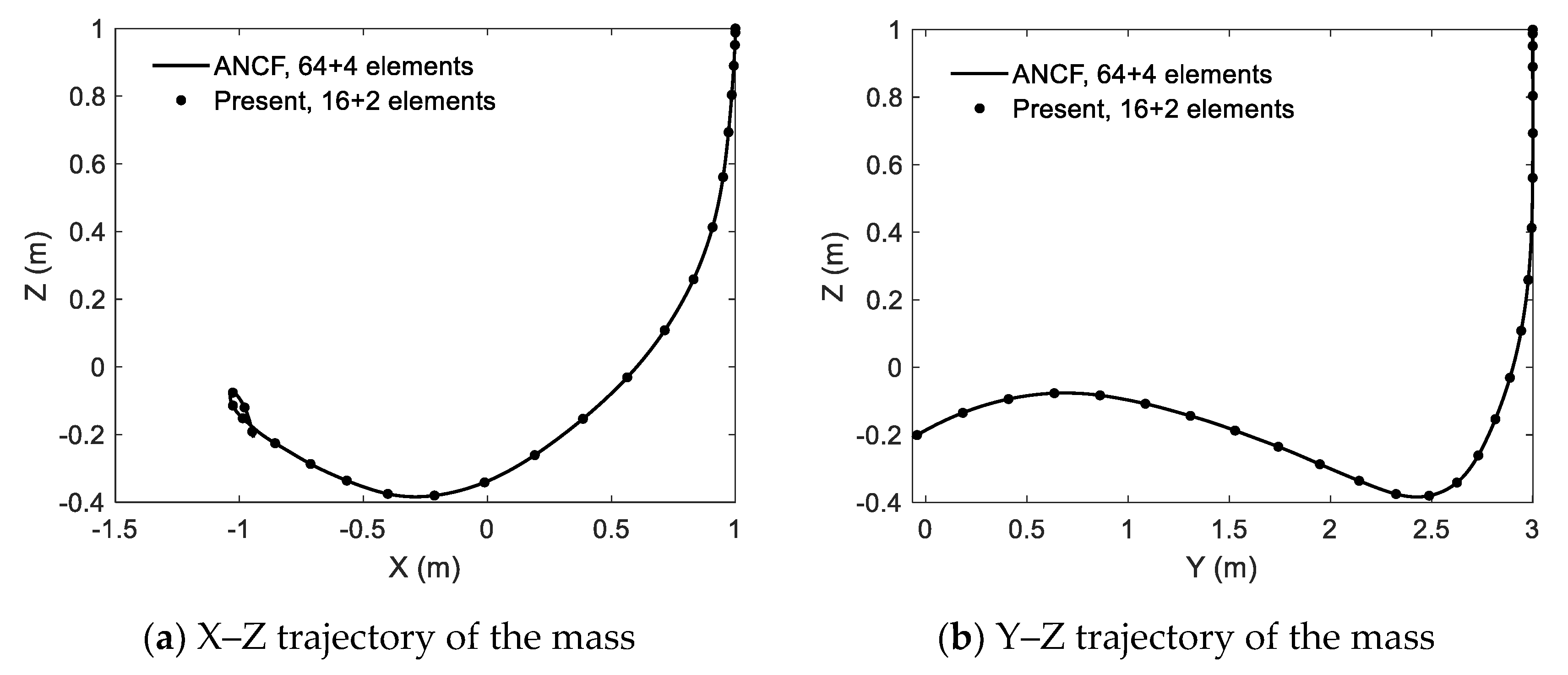
5.2. Sliding Three-Dimensional Beam with Eccentricity

Two initial straight flexible beams connected through a sliding joint are involved in this example, as shown in Figure 4. Two spherical joints locate at the two ends of the carrier beam AB. A concentrated mass M is fixed at the free end of sliding beam AM. All the geometrical and material parameters are displayed in

Table 3. Parameters for the carrier beam, sliding beam, and mass.

Parameters	Value
Position of A	[0,3,1]
Position of B	[0,0,0]
Position of M	[1,3,1]
Cross-section	(0.01 × 0.01) m2
Young’s modulus	2e8 N/m2
Poisson coefficient	0.3
Mass density	800 kg/m3
Tip mass	1 kg
Gravity	9.81 m/s2

. This is a typical test case of sliding joint, which has been proposed by Sugiyama et al. [19] and applied by other researchers [20,23]. The ANCF and GEBT are employed in [19,20] and [23], respectively. In reference [19,23], the carrier beam and sliding beam are both discretized into one element thereby obtaining an un-converged solution. The convergence of solution was investigated in [23].

In the example, the carrier beam and sliding beam are discretized into 16 and 2 elements using the 2-order NURBS basic function. For comparison, the reference solutions from ANCF with 64 and 4 elements were calculated. The calculation was conducted with the time step h = 0.001 s and terminated once the sliding beam reaches point B, which occurred at t = 1.306 s. The deformed configurations during the motion are shown in Figure 5 with the time interval Δt = 0.1 s, while the X–Z and Y–Z trajectories of the mass are plotted in Figure 6. It is shown that the flexible beams have visible deformation during the finite translational and rotational process. The results from the present method have a good agreement with the reference solution from ANCF. It is demonstrated that the present formulation is applicable to the analysis of the structures with sliding joint, which undergo finite deformation and motion.

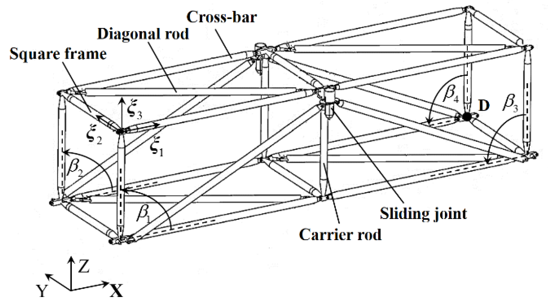
5.3. Deployable Spatial Truss Structure Unit

The dynamics of a deployable truss structure unit, which can be employed to construct large space systems [34], was investigated in this section. As shown in Figure 7, the structure unit is an assembly composed of three square frames, eight cross-bars, and eight diagonal rods joined to one another. The cross-bars and the diagonal rods on both sides are jointed with square frames with only the rotations around the ${\xi }_2$-axis released, while the above and below diagonal rods are clamped at corresponding points on square frames. During the deployment process, the diagonal rods on both sides can slide between two ends of the carrier rods through a sliding joint. The geometrical and material parameters can be found in

Table 4. Parameters for the deployable truss structure unit.

Parameters	Value
Side length of square frame	2 m
Length of cross-bar	4 m
Length of diagonal rod	$\sqrt{20}$ m
Inside diameter of all rods	0.055 m
Outside diameter of all rods	0.060 m
Young’s modulus	2.1e11 N/m2
Poisson coefficient	0.3
Mass density	7850 kg/m3
Gravity	9.81 m/s2

.

In the first test case, the first (left) square frame was fixed initially, and the structure unit was kept with ${\beta }_i$ = 5° (i = 1, 2, 3, 4). Then, the structure unit was driven with the gravity 0.005 g along X-axis. The calculation was conducted with the time step h = 0.1 s and a single 2-order NURBS finite element per beam. When ${\beta }_i$ = 90° (i = 1, 2, 3, 4), as shown in Figure 7, the sliding joints were locked in the top end of carrier beams, and the calculation was terminated through a constraint of ζ. For comparison, the reproductive simulation based on MSC.ADAMS and ANSYS were conducted. As suggested by [35,36], the modal neutral files (.mnf files) was firstly obtained from ANSYS and was then imported into ADAMS/FLEX module, which allows us to model flexible parts based on its modal frequency. The beam members were modeled with the specified parameters in Table 4 using Solid45 element in ANSYS. The X-position of point D during the motion calculated from proposed formulation were of good agreement with MSC.ADAMS, as displayed in Figure 8. It was demonstrated that the present formulation was appropriate for the deployment dynamic analysis of the spatial truss structure.

In the second case, the initial configuration and material parameters were the same with the first case, while the gravity was ignored. The structure was set to deploy in $t_f$ = 20 s through control function applied in ${\beta }_i$ (i = 1, 2, 3, 4) synchronously with the time step h = 0.005 s, and the simulation was terminated at 30 s. Equations (54)–(57) are the linear control function, polynomial control function, cycloid control function, and cosine control function with ${\beta }_0$ = 5°, ${\beta }_f$ = 90°, respectively.

$${\beta }_i(t)=({\beta }_f-{\beta }_0)\frac{t}{t_f}(i=1,2,3,4)$$

(54)

$${\beta }_i(t)=({\beta }_f-{\beta }_0)[6{(\frac{t}{t_f})}^5-15{(\frac{t}{t_f})}^4+10{(\frac{t}{t_f})}^3]+{\beta }_0(i=1,2,3,4)$$

(55)

$${\beta }_i(t)=({\beta }_f-{\beta }_0)[\frac{t}{t_f}-\frac{1}{2\pi }\sin (\frac{2\pi t}{t_f})]+{\beta }_0(i=1,2,3,4)$$

(56)

$${\beta }_i(t)=({\beta }_f-{\beta }_0)[\frac{1}{2}-\frac{9}{16}\cos (\frac{\pi t}{t_f})+\frac{1}{16}\cos (\frac{3\pi t}{t_f})]+{\beta }_0(i=1,2,3,4)$$

(57)

To test the convergence of element, 4 and 10 finite elements using 2-order NURBS basic function were employed at first. As displayed in Figure 9, the motions of D in X direction obtained from two discrete ways agreed well, which demonstrated that the results had converged. Note that the following tests were all conducted with four finite elements. The motions of D in X direction and Z direction calculated by four control functions are displayed in Figure 10 and Figure 11. The results from linear control function show visible vibration whether in the deployment process or after the deployment. This is because the initial increment set by the linear function is too large, which causes a larger elastic deformation and results in an unsmooth deployment. The comparison result in Z-position of point D from other three angle control functions is plotted in Figure 12. It is illustrated that the cosine function is the best control strategies in four functions, since it shows the best deployment stability and minimum residual vibration after the deployment.

6. Conclusions

In order to investigate the dynamics of the deployable spatial truss structure, a beam finite element that can effectively reduce the rotational nonlinearity thereby applicable for finite motion and deformation issues, was proposed based on the geometrically exact beam theory and the local frame approach. The analytical expressions of internal and inertial forces and their Jacobian matrices, including the symmetric stiffness matrix, were strictly derived in this paper. Based on the Lagrangian multiplier method, the constraint equation and its Jacobian matrix of sliding joint were also derived. Using NURBS basic function, the displacement and rotation fields were interpolated separately to be compatible with IGA. The numerical example illustrated that the iteration matrix corresponding to the rotational parameters in the initial configuration, including the Jacobian matrix of inertial and internal forces, could be maintained in the whole simulation, which drastically improved the computational efficiency. Moreover, the sliding joint was also successfully tested. The application example demonstrated that the present method was applicable to the deployable truss structure with sliding joint. The simulation results show that the effect of the cosine function on angle planning was better than the linear function, polynomial function, and cycloid function.

References

1. Shabana, A.A. Definition of the slopes and the finite element absolute nodal coordinate formulation. Multibody Sys. Dyn. 1997, 1, 339–348. [Google Scholar] [CrossRef]
2. Shabana, A.A.; Yakoub, R.Y. Three dimensional absolute nodal coordinate formulation for beam elements: Theory. J. Mech. Des. 2001, 123, 606–613. [Google Scholar] [CrossRef]
3. Romero, I. A comparison of finite elements for nonlinear beams: The absolute nodal coordinate and geometrically exact formulations. Multibody Sys. Dyn. 2008, 20, 51–68. [Google Scholar] [CrossRef] [Green Version]
4. Bauchau, O.A.; Han, S.; Mikkola, A.; Matikainen, M.K. Comparison of the absolute nodal coordinate and geometrically exact formulations for beams. Multibody Sys. Dyn. 2013, 32, 67–85. [Google Scholar] [CrossRef]
5. Reissner, E. On one-Dimensional finite-Strain beam theory: The plane problem. Appl. Math. Phys. 1972. [Google Scholar] [CrossRef]
6. Reissner, E. On one-Dimensional large displacement finite strain beam theory. Stud. Appl. Math. 1973. [Google Scholar] [CrossRef]
7. Simo, J.C. A finite strain beam formulation. The three-dimensional dynamic problem. Part I. Comput. Methods Appl. Mech. Engrg. 1985, 49, 55–70. [Google Scholar] [CrossRef]
8. Simo, J.C.; Vu-Quoc, L. A three-Dimensional finite-Strain rod model. Part ii: Computational aspects. Comput. Methods Appl. Mech. Engrg. 1986, 58, 79–116. [Google Scholar] [CrossRef]
9. Simo, J.C.; Vu-Quoc, L. On the dynamics in space of rods undergoing large motions—A geometrically exact approach. Comput. Methods Appl. Mech. Engrg. 1988, 66, 125–161. [Google Scholar] [CrossRef]
10. Cardona, A.; Géradin, M. A beam finite element non-linear theory with finite rotations. Int. J. Numer. Methods Eng. 1988, 26, 2403–2438. [Google Scholar] [CrossRef]
11. Ibrahimbegović, A.; Frey, F.; Kozar, I. Computational aspects of vector-Like parametrization of 3-dimensional finite rotations. Int. J. Numer. Methods Eng. 1995, 38, 3653–3673. [Google Scholar] [CrossRef]
12. Crisfield, M.A.; Jelenić, G. Objectivity of strain measures in the geometrically exact three-Dimensional beam theory and its finite-Element implementation. Proc. R. Soc. Lond. Ser. A Math. Phys. Eng. Sci. 1999, 455, 1125–1147. [Google Scholar] [CrossRef]
13. Jelenić, G.; Crisfield, M.A. Geometrically exact 3d beam theory: Implementation of a strain-Invariant finite element for statics and dynamics. Comput. Methods Appl. Mech. Engrg. 1999, 171, 141–171. [Google Scholar] [CrossRef]
14. Romano, G.; Barretta, R.; Diaco, M. Geometric continuum mechanics. Meccanica 2014, 49, 111–133. [Google Scholar] [CrossRef]
15. Romano, G.; Barretta, R.; Diaco, M. The geometry of nonlinear elasticity. Acta Mech. 2014, 225, 3199–3235. [Google Scholar] [CrossRef] [Green Version]
16. Shigley, J.E.; Uicker, J.J. Theory of Machines and Mechanisms; McGrawHill: New York, NY, USA, 1980. [Google Scholar] [CrossRef] [Green Version]
17. Bauchau, O.A. On the modeling of prismatic joints in flexible multi-Body systems. Comput. Methods Appl. Mech. Engrg. 2000, 181, 87–105. [Google Scholar] [CrossRef]
18. Bauchau, O.A.; Bottasso, C.L. Contact conditions for cylindrical, prismatic, and screw joints in flexible multibody systems. Multibody Syst. Dyn. 2001, 5, 251–278. [Google Scholar] [CrossRef]
19. Sugiyama, H.; Escalona, J.L.; Shabana, A.A. Formulation of three-Dimensional joint constraints using the absolute nodal coordinates. Nonlinear Dyn. 2003, 31, 167–195. [Google Scholar] [CrossRef]
20. Gerstmayr, J.; Shabana, A.A. Analysis of thin beams and cables using the absolute nodal co-Ordinate formulation. Nonlinear Dyn. 2006, 45, 109–130. [Google Scholar] [CrossRef]
21. García de Jalón, J.; Bayo, E. Inematic and Dynamic Simulation of Multibody Systems––The Real-Time Challenge; Springer: New York, NY, USA, 1994. [Google Scholar] [CrossRef]
22. Géradin, M.; Cardona, A. A finite element approach. In Flexible Multibody Dynamics; John Wiley & Sons: Hoboken, NJ, USA, 2001. [Google Scholar]
23. Munoz, J.J.; Jelenić, G. Sliding contact conditions using the master-Slave approach with application on geometrically non-Linear beams. Int. J. Solids Struct. 2004, 41, 6963–6992. [Google Scholar] [CrossRef] [Green Version]
24. Hughes, T.J.R.; Cottrell, J.A.; Bazilevs, Y. Isogeometric analysis: Cad, finite elements, NURBS, exact geometry and mesh refinement. Comput. Methods Appl. Mech. Engrg. 2005, 194, 4135–4195. [Google Scholar] [CrossRef] [Green Version]
25. De Lorenzis, L.; Wriggers, P.; Hughes, T.J.R. Isogeometric contact: A review. GAMM-Mitt. 2014, 37, 85–123. [Google Scholar] [CrossRef]
26. Bauer, A.M.; Breitenberger, M.; Philipp, B.; Wüchner, R.; Bletzinger, K.U. Nonlinear isogeometric spatial bernoulli beam. Comput. Methods Appl. Mech. Engrg. 2016, 303, 101–127. [Google Scholar] [CrossRef]
27. Greco, L.; Cuomo, M. An isogeometric implicit g (1) mixed finite element for kirchhoff space rods. Comput. Methods Appl. Mech. Engrg. 2016, 298, 325–349. [Google Scholar] [CrossRef]
28. Choi, M.-J.; Yoon, M.; Cho, S. Isogeometric configuration design sensitivity analysis of finite deformation curved beam structures using jaumann strain formulation. Comput. Methods Appl. Mech. Engrg. 2016, 309, 41–73. [Google Scholar] [CrossRef]
29. Choi, M.-J.; Cho, S. Isogeometric configuration design sensitivity analysis of geometrically exact shear-Deformable beam structures. Comput. Methods Appl. Mech. Engrg. 2019, 351, 153–183. [Google Scholar] [CrossRef]
30. Arnold, M.; Bruls, O. Convergence of the generalized-alpha scheme for constrained mechanical systems. Multibody Sys. Dyn. 2007, 18, 185–202. [Google Scholar] [CrossRef]
31. Brüls, O.; Cardona, A.; Arnold, M. Lie group generalized-α time integration of constrained flexible multibody systems. Mech. Mach. Theory 2012, 48, 121–137. [Google Scholar] [CrossRef]
32. Argyris, J. An excursion into large rotations. Comput. Methods Appl. Mech. Engrg. 1982, 32, 85–155. [Google Scholar] [CrossRef]
33. Bauchau, O.A. Flexible Multibody Dynamics; Springer: Dordrecht, The Netherlands, 2011. [Google Scholar] [CrossRef]
34. Li, W.; Cheng, D.; Liu, X.; Wang, Y.; Shi, W.; Tang, Z.; Gao, F.; Zeng, F.; Chai, H.; Luo, W.; et al. On-Orbit service (OOS) of spacecraft: A review of engineering developments. Prog. Aerosp. Sci. 2019, 108, 32–120. [Google Scholar] [CrossRef]
35. Zhang, J.; Zhong, J.; He, L.; Gao, R. Modal analysis of the cable-Stayed space truss combining ansys and msc.adams. Adv. Mater. Res. 2010, 121–122, 832–837. [Google Scholar] [CrossRef]
36. Luo, H.; Chen, Z.; Leng, Y.; Wang, H. Rigid-Flexible coupling dynamics simulation of 3-rps parallel robot based on adams and ansys. Appl. Mech. Mater. 2013, 290, 91–96. [Google Scholar] [CrossRef]
Figure 1. Initial configuration and the current configuration.
Applsci 10 01231 g001
Figure 2. The configuration of the slider-crank.
Applsci 10 01231 g002
Figure 3. The deformation rate of Rod II.
Applsci 10 01231 g003
Figure 4. The initial configuration of the test case.
Applsci 10 01231 g004
Figure 5. The deformed configurations during the motion with Δt = 0.1s.
Applsci 10 01231 g005
Figure 6. The trajectories of the mass displayed in different planes: (a) X–Z plane and (b) Y–Z plane.
Applsci 10 01231 g006
Figure 7. The deployed configuration of the structure unit.
Applsci 10 01231 g007
Figure 8. The X-position of point D.
Applsci 10 01231 g008
Figure 9. The X-position of point D from 10 elements and 4 elements using linear control function.
Applsci 10 01231 g009
Figure 10. The X-position of point D from different angle control functions.
Applsci 10 01231 g010
Figure 11. The Z-position of point D from different angle control functions.
Applsci 10 01231 g011
Figure 12. The Z-position of point D from three angle control functions.
Applsci 10 01231 g012