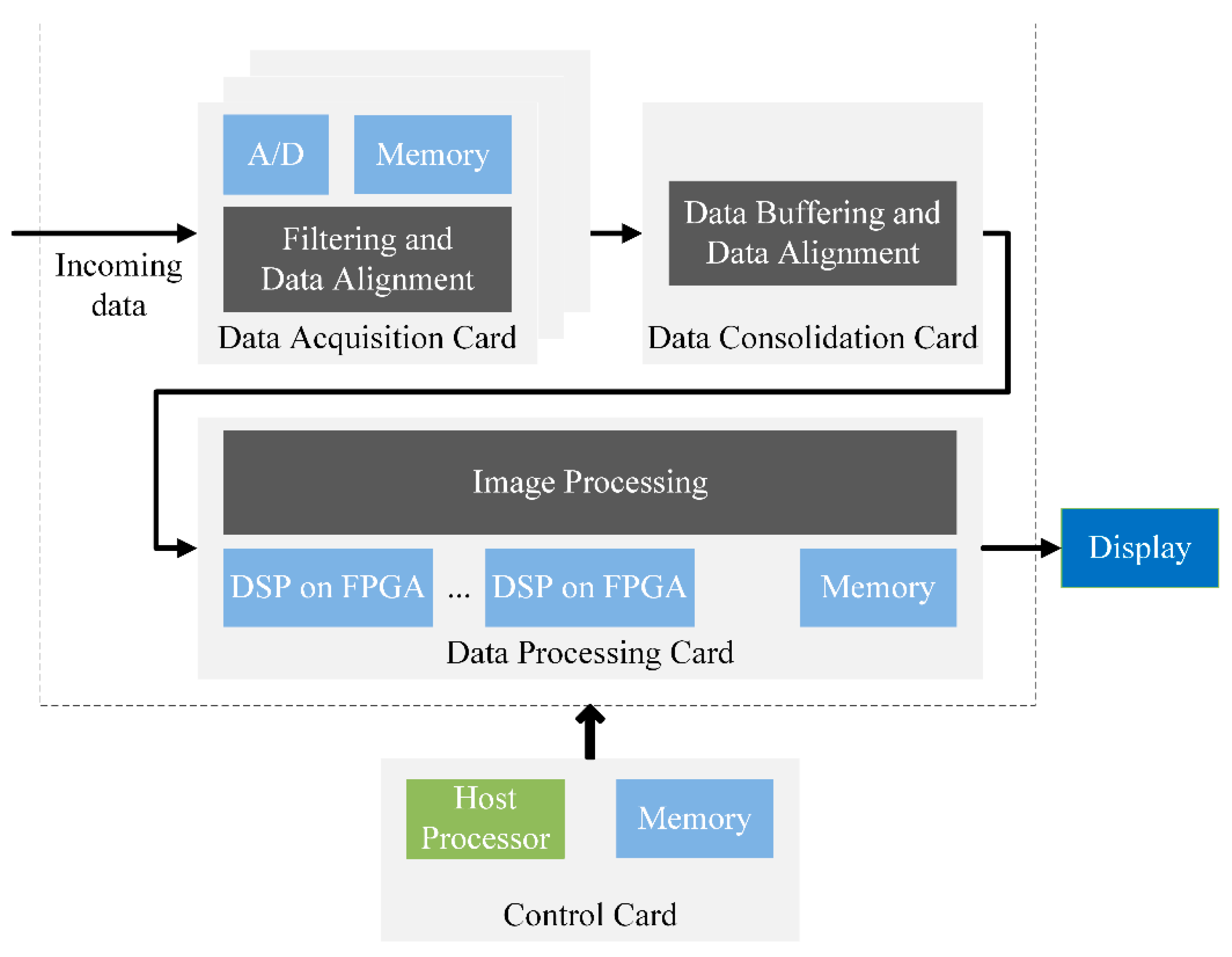
Figure 1.
The typical medical imaging system.
Figure 1.
The typical medical imaging system.
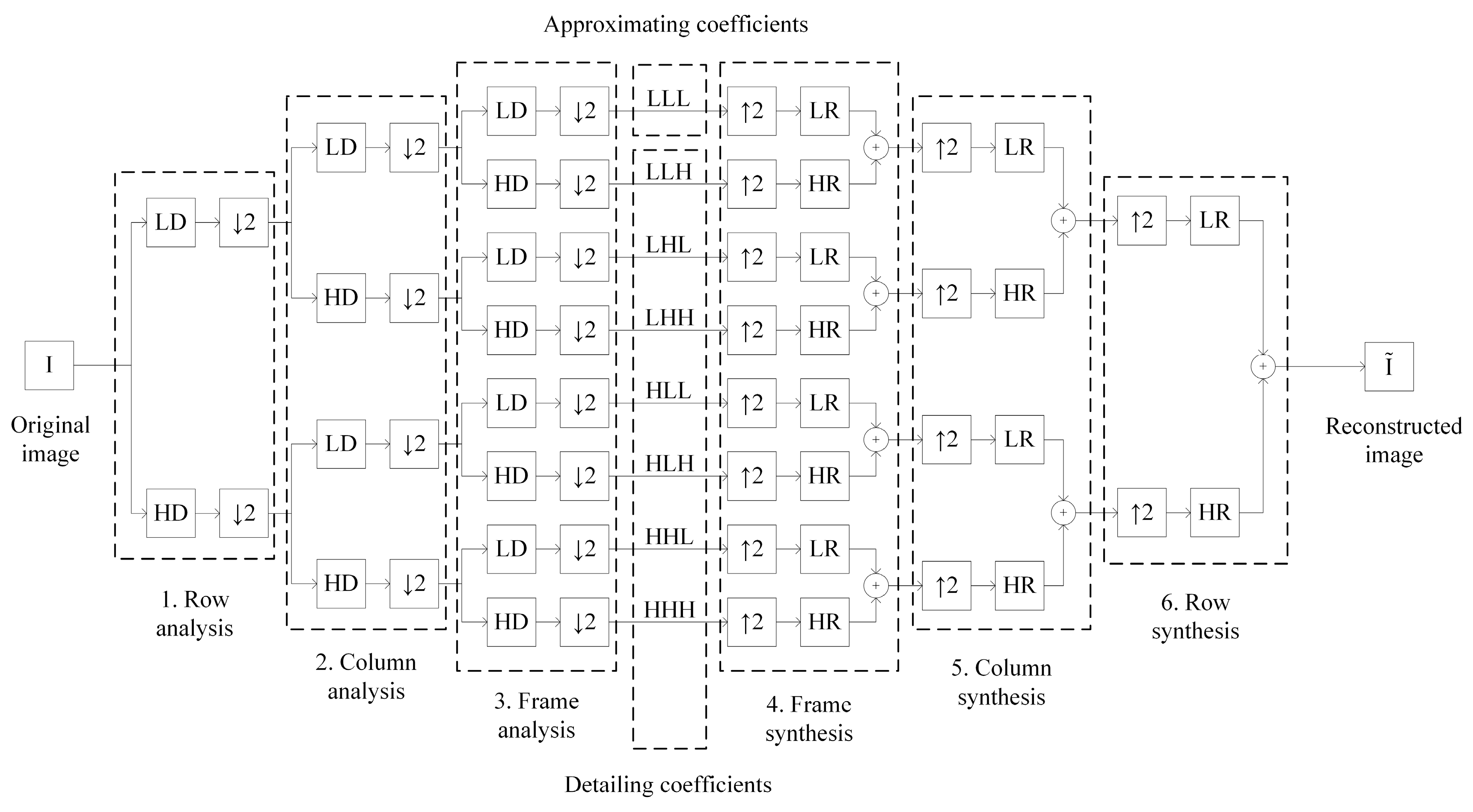
Figure 2.
The scheme of 3D image discrete wavelet transform (DWT).
Figure 2.
The scheme of 3D image discrete wavelet transform (DWT).
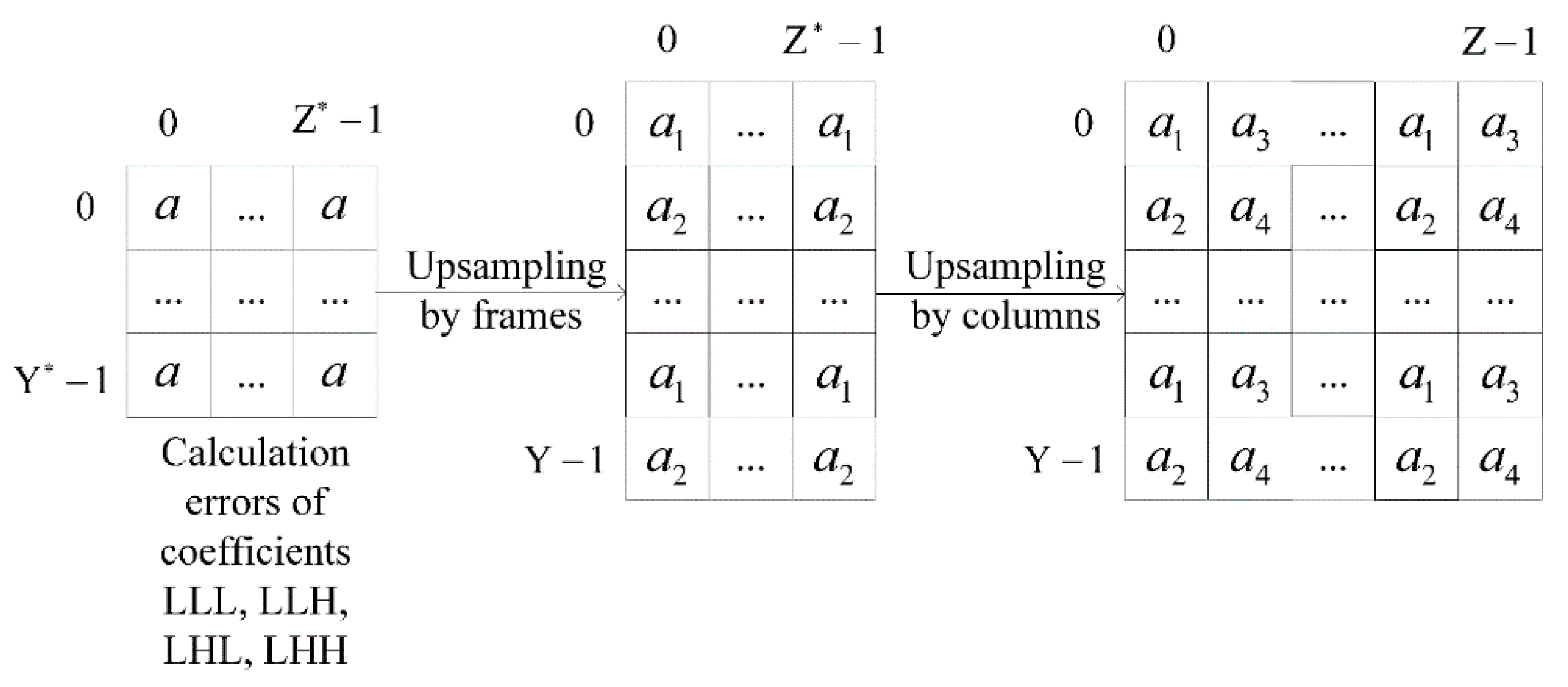
Figure 3.
The scheme of the errors separation with upsampling by frames and columns.
Figure 3.
The scheme of the errors separation with upsampling by frames and columns.
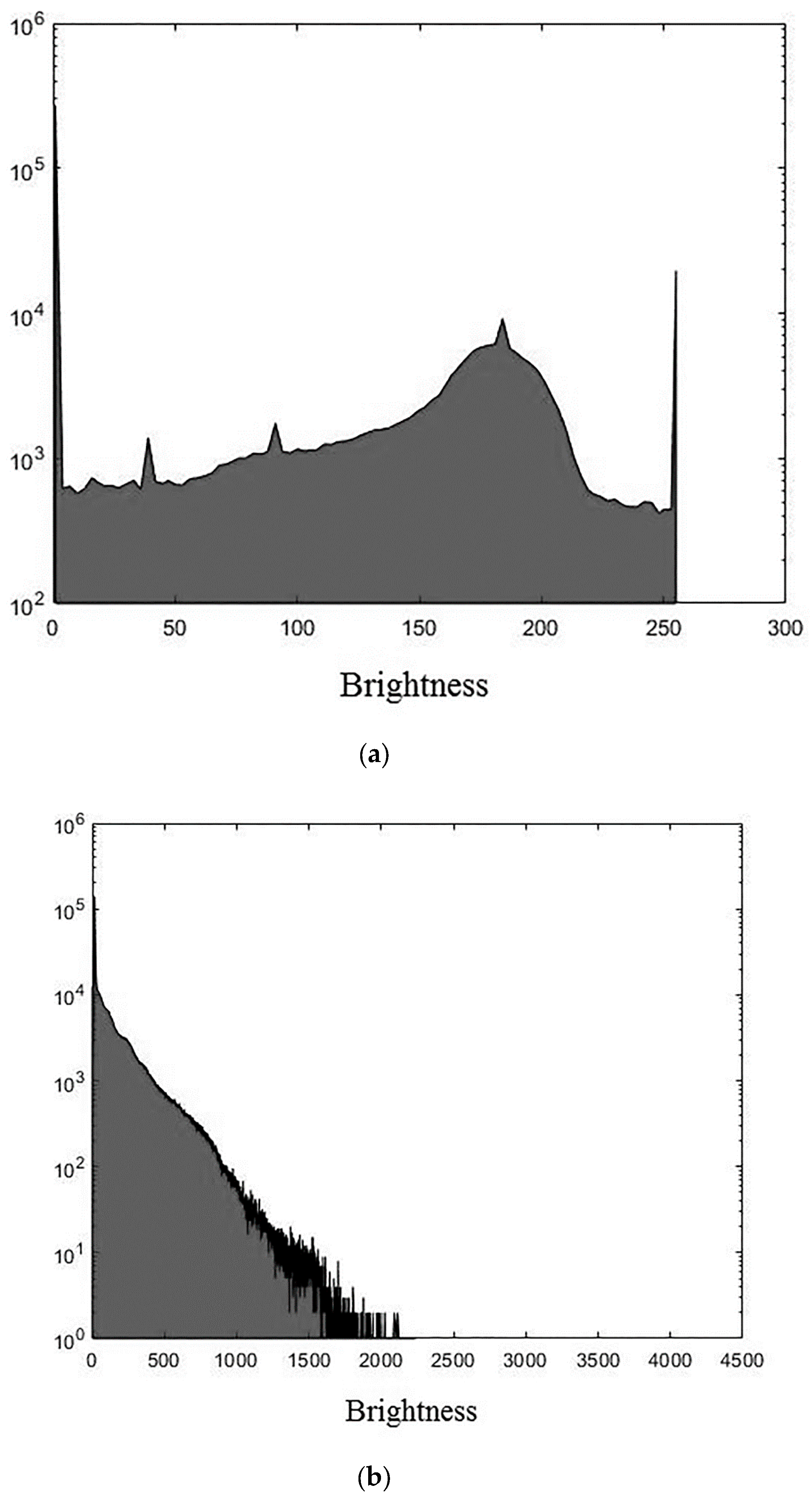
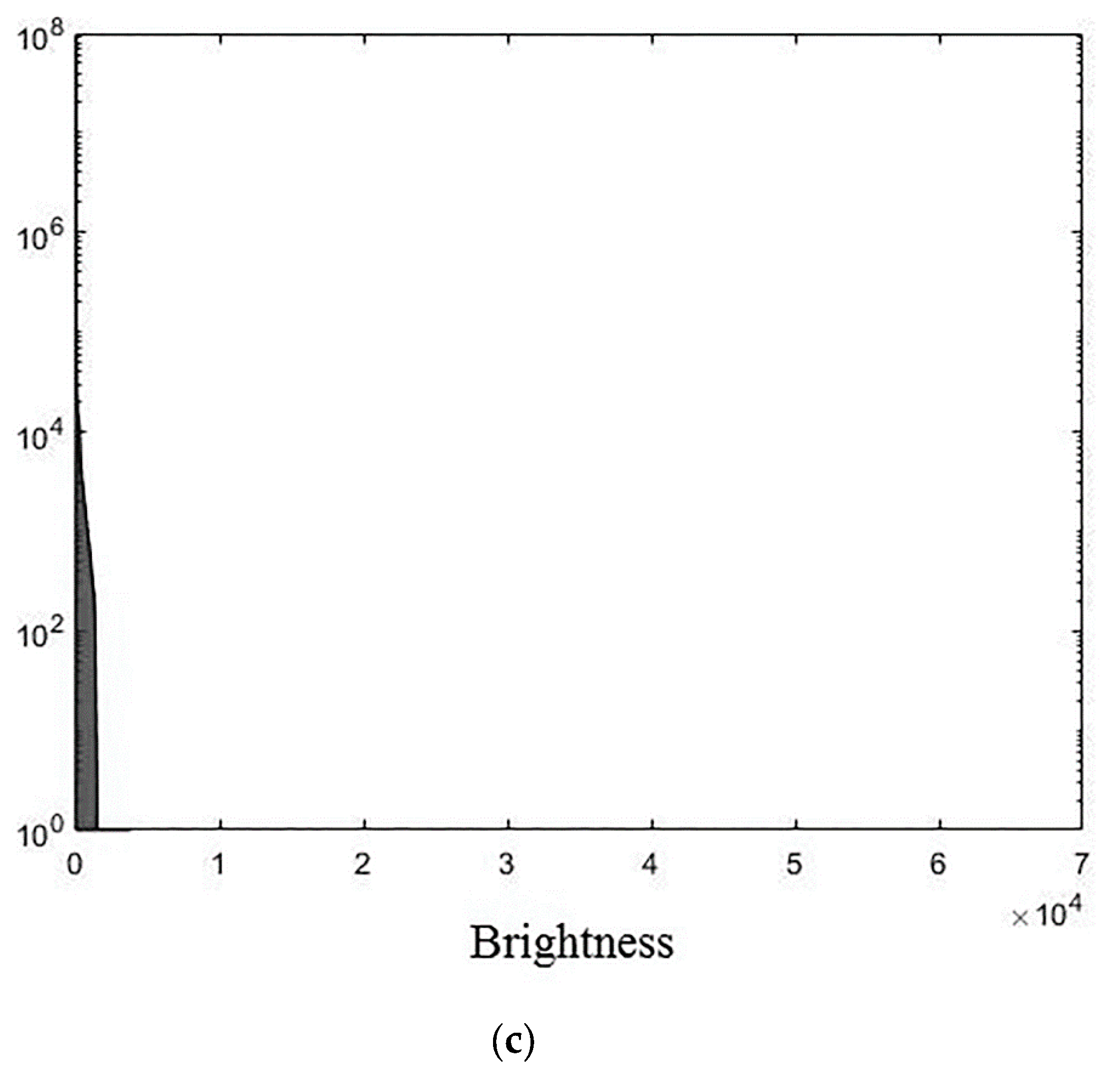
Figure 4.
Histograms of used images: (a) “wmri”, average brightness ; (b) “Trufi_COR”, average brightness and (c) “Body_1.0”, average brightness .
Figure 4.
Histograms of used images: (a) “wmri”, average brightness ; (b) “Trufi_COR”, average brightness and (c) “Body_1.0”, average brightness .
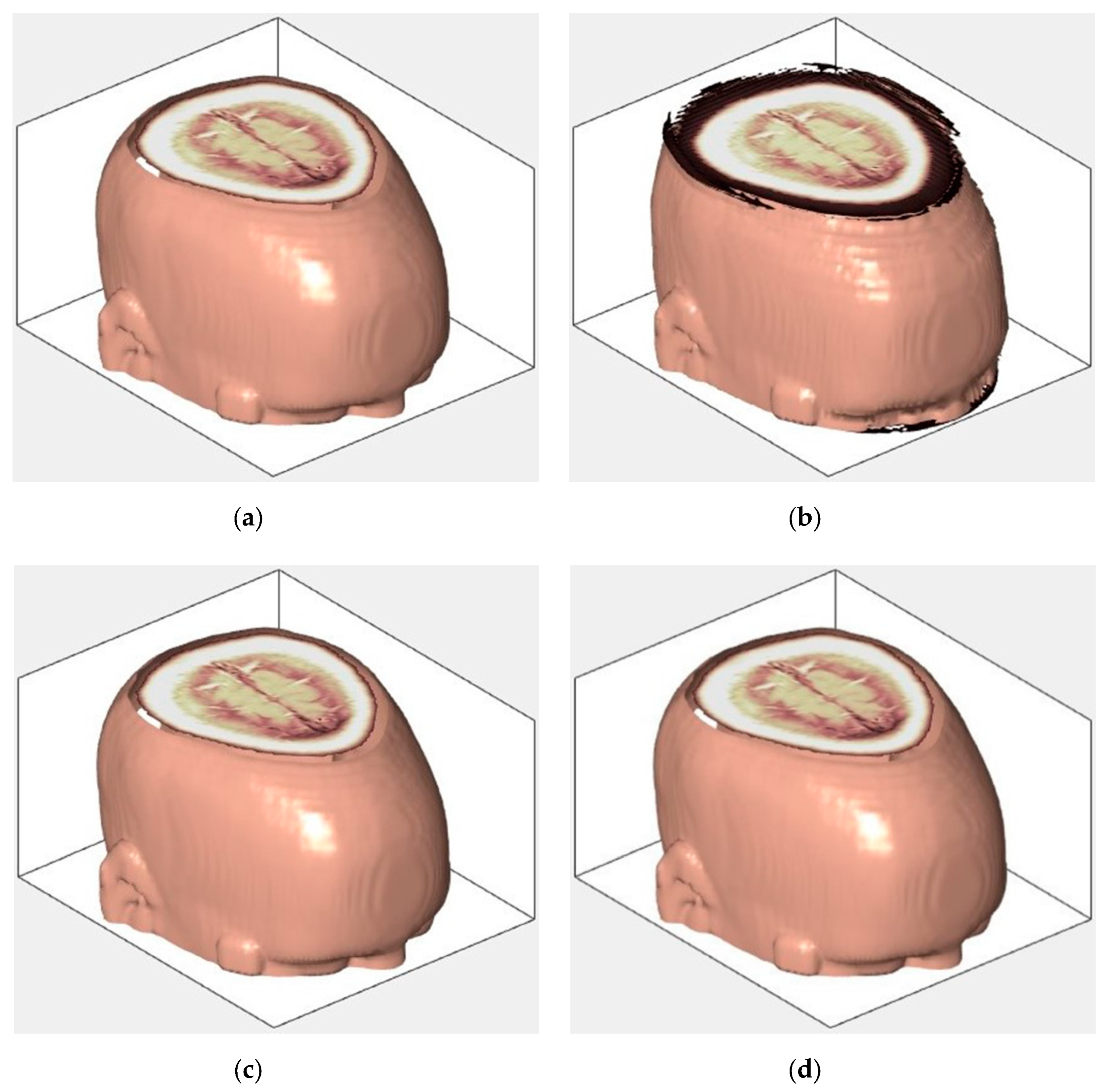
Figure 5.
Example of 3D tomographic 8-bit image “wmri” DWT by wavelet: (a) original image; processed image: (b) , dB; (c) , dB and (d) , .
Figure 5.
Example of 3D tomographic 8-bit image “wmri” DWT by wavelet: (a) original image; processed image: (b) , dB; (c) , dB and (d) , .
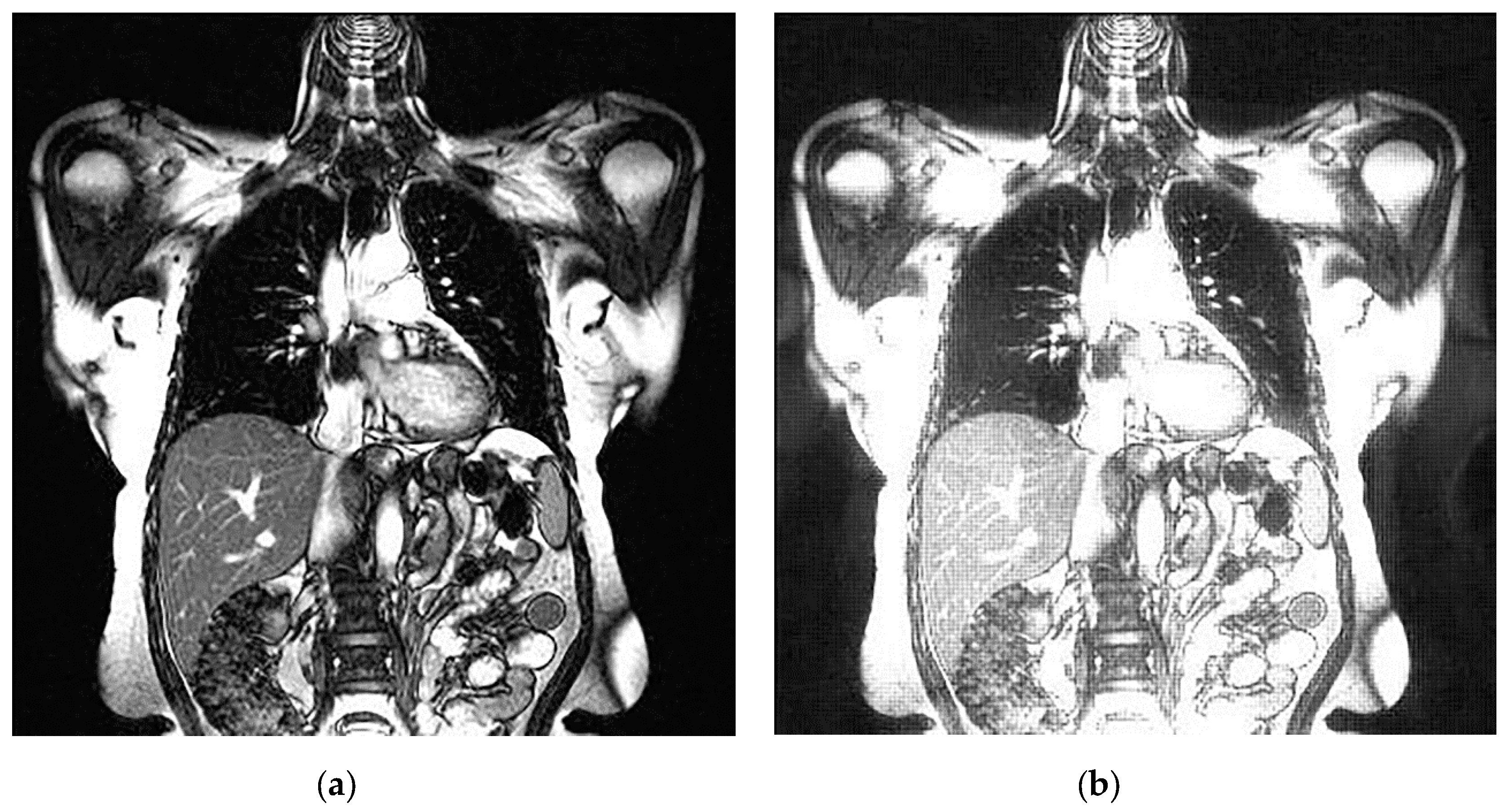
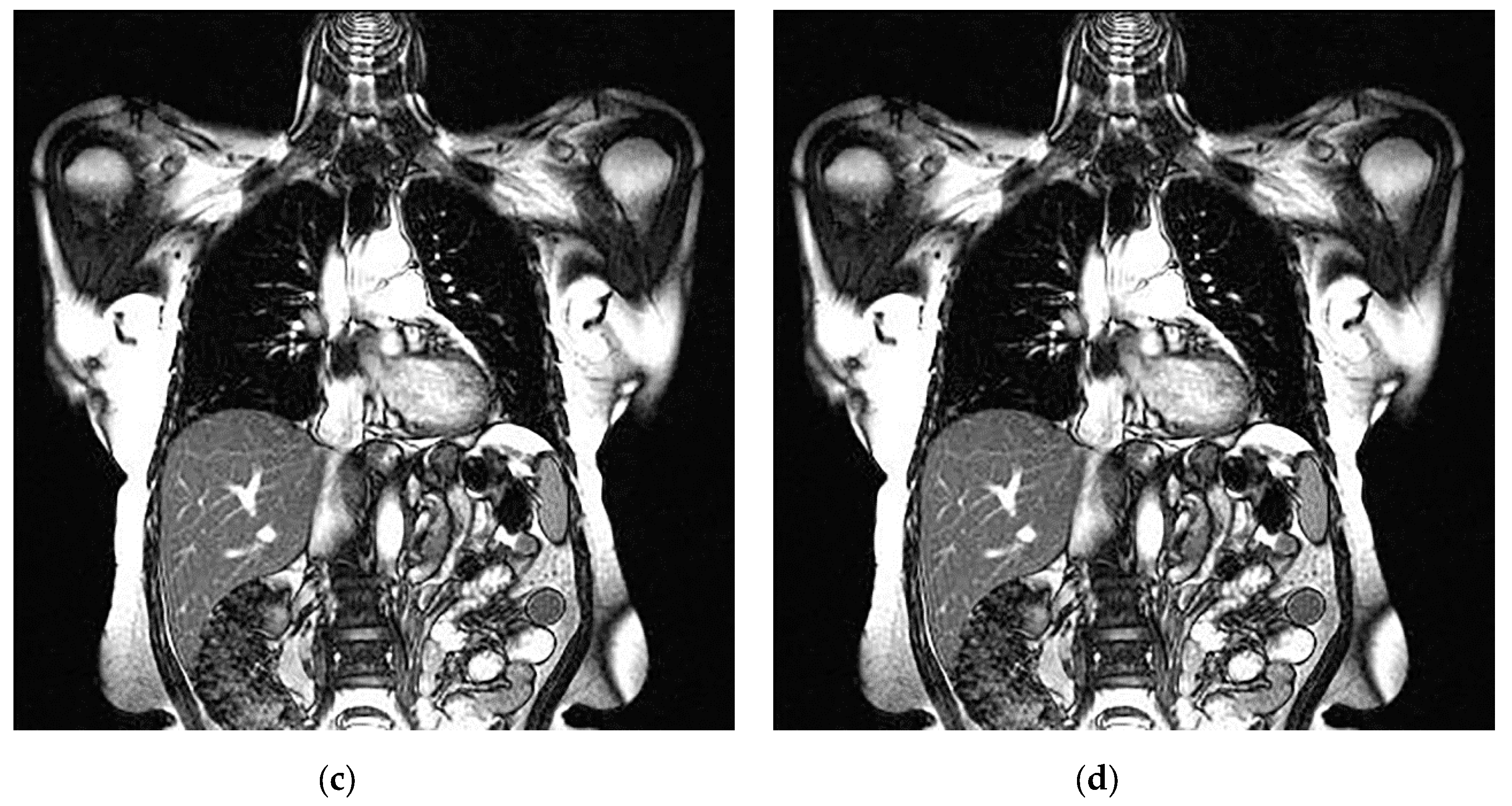
Figure 6.
Example of 3D tomographic 12-bit image “Trufi_COR” (15-th frame) DWT by wavelet: (a) original image; processed image: (b) , dB; (c) , dB and (d) , .
Figure 6.
Example of 3D tomographic 12-bit image “Trufi_COR” (15-th frame) DWT by wavelet: (a) original image; processed image: (b) , dB; (c) , dB and (d) , .
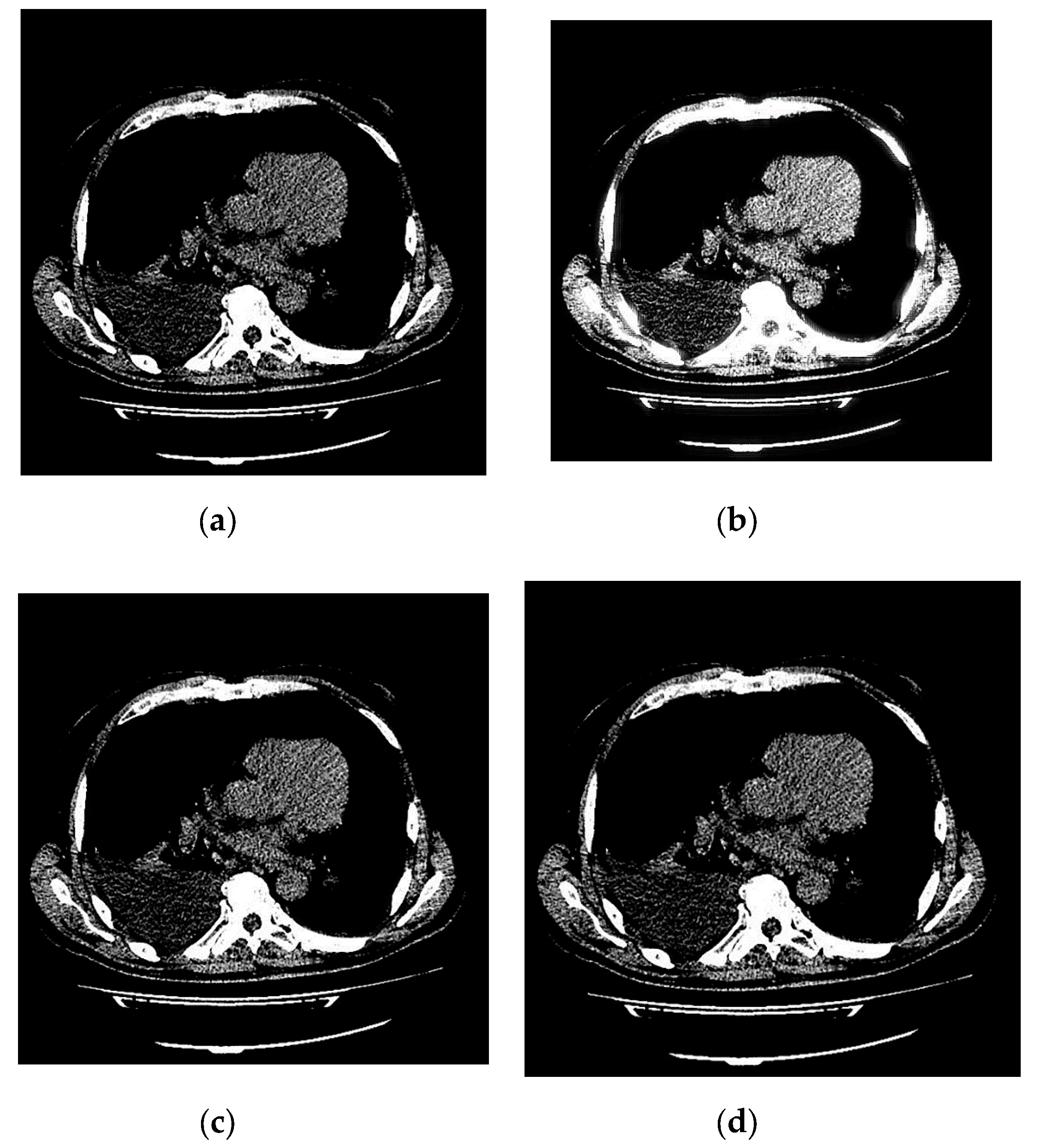
Figure 7.
Example of 3D tomographic 16-bit image “Body_1.0” (1-st frame) DWT by wavelet: (a) original image; processed image: (b) , dB; (c) , dB and (d) , .
Figure 7.
Example of 3D tomographic 16-bit image “Body_1.0” (1-st frame) DWT by wavelet: (a) original image; processed image: (b) , dB; (c) , dB and (d) , .
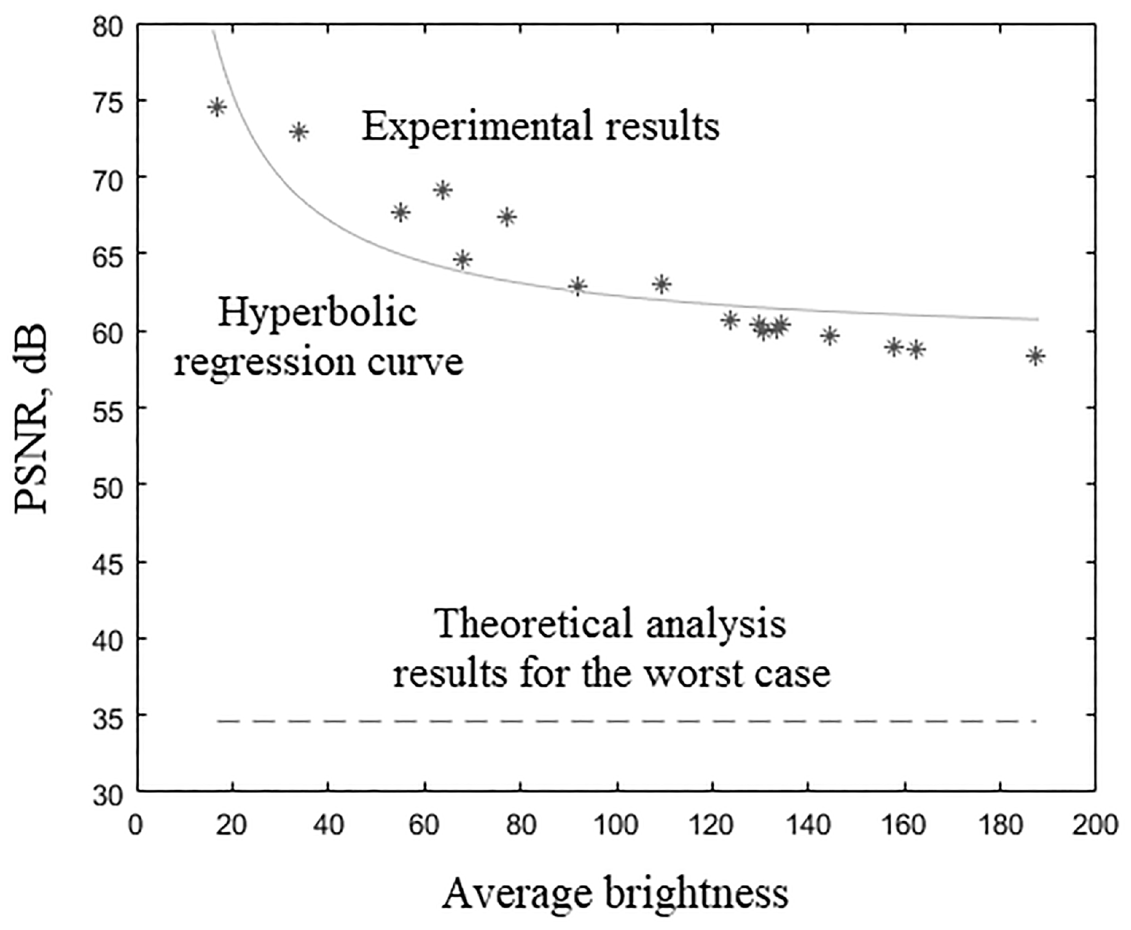
Figure 8.
Experimental results of 3D tomographic 12-bit images DWT by wavelet with bit-width of filters coefficients.
Figure 8.
Experimental results of 3D tomographic 12-bit images DWT by wavelet with bit-width of filters coefficients.
Table 1.
Calculation results (, dB) of 3D medical images (with 8 BPC) DWT by using bit-width of Daubechies wavelets filters coefficients.
Table 1.
Calculation results (, dB) of 3D medical images (with 8 BPC) DWT by using bit-width of Daubechies wavelets filters coefficients.
| | | | | | | | | | |
|---|
| 10 | 36.79 | 36.67 | 29.87 | 30.08 | 31.59 | 24.60 | 22.29 | 24.46 | 22.19 | 22.08 |
| 11 | 44.15 | 43.36 | 39.68 | 34.58 | 36.67 | 32.22 | 28.80 | 31.17 | 28.58 | 27.60 |
| 12 | 57.16 | 48.71 | 44.15 | 41.85 | 43.36 | 39.68 | 34.58 | 37.82 | 35.26 | 35.34 |
| 13 | | | 51.14 | 51.14 | 51.14 | 47.16 | 43.18 | 43.36 | 43.36 | 39.68 |
| 14 | | | | | | 57.16 | 51.14 | 51.14 | 51.14 | 47.16 |
| 15 | | | | | | | | | | |
Table 2.
Calculation results (, dB) of 3D medical images (with 12 BPC) DWT by using bit-width of Daubechies wavelets filters coefficients.
Table 2.
Calculation results (, dB) of 3D medical images (with 12 BPC) DWT by using bit-width of Daubechies wavelets filters coefficients.
| | | | | | | | | | |
|---|
| 12 | 49.43 | 45.01 | 42.18 | 40.05 | 41.80 | 38.21 | 33.76 | 36.69 | 34.47 | 34.40 |
| 13 | 57.46 | 52.38 | 49.10 | 46.76 | 46.46 | 44.76 | 41.11 | 41.99 | 41.92 | 39.07 |
| 14 | 71.28 | 61.23 | 54.39 | 52.38 | 52.27 | 50.35 | 47.91 | 47.73 | 47.65 | 44.90 |
| 15 | 70.86 | 71.28 | 61.11 | 59.15 | 57.68 | 57.46 | 55.52 | 52.38 | 53.27 | 52.27 |
| 16 | | 81.28 | 71.28 | 64.37 | 63.79 | 63.79 | 63.15 | 57.97 | 59.85 | 56.33 |
| 17 | | | | 70.86 | 75.26 | 71.28 | 68.49 | 67.30 | 64.37 | 63.79 |
| 18 | | | | | 81.28 | 81.28 | 75.26 | 75.26 | 75.26 | 71.28 |
| 19 | | | | | | | | | | 81.28 |
| 20 | | | | | | | | | | |
Table 3.
Calculation results (, dB) of 3D medical images (with 16 BPC) DWT by using bit-width of Daubechies wavelets filters coefficients.
Table 3.
Calculation results (, dB) of 3D medical images (with 16 BPC) DWT by using bit-width of Daubechies wavelets filters coefficients.
| | | | | | | | | | |
|---|
| 16 | 77.35 | 76.55 | 67.85 | 63.56 | 61.94 | 63.27 | 61.70 | 57.52 | 59.24 | 55.92 |
| 17 | 93.90 | 77.35 | 76.91 | 68.05 | 71.33 | 67.85 | 66.49 | 65.34 | 63.50 | 62.62 |
| 18 | 102.35 | 88.73 | 80.42 | 77.35 | 75.56 | 73.79 | 71.69 | 71.42 | 71.36 | 69.35 |
| 19 | 105.36 | 95.36 | 85.19 | 86.02 | 81.76 | 81.86 | 78.48 | 76.46 | 78.34 | 75.56 |
| 20 | | 99.34 | 92.35 | 91.56 | 90.05 | 87.96 | 85.19 | 83.84 | 84.87 | 83.46 |
| 21 | | | 99.34 | 105.36 | 99.34 | 99.34 | 92.57 | 91.38 | 93.45 | 87.88 |
| 22 | | | | | 105.36 | | 105.36 | 99.34 | 105.36 | 95.36 |
| 23 | | | | | | | | | | 105.36 |
| 24 | | | | | | | | | | |
Table 4.
Calculation results (, dB) of 3D medical images (with 8 BPC) DWT by using bit-width of symlets filters coefficients.
Table 4.
Calculation results (, dB) of 3D medical images (with 8 BPC) DWT by using bit-width of symlets filters coefficients.
| | | | | | | | | | |
|---|
| 10 | 36.79 | 36.67 | 29.87 | 30.08 | 26.15 | 26.07 | 24.53 | 24.46 | 21.15 | 22.08 |
| 11 | 44.15 | 43.36 | 39.68 | 34.58 | 32.46 | 32.22 | 30.83 | 31.17 | 26.75 | 26.15 |
| 12 | 57.16 | 48.71 | 44.15 | 41.85 | 41.85 | 36.99 | 35.04 | 37.82 | 34.71 | 32.46 |
| 13 | | | 51.14 | 51.14 | 51.14 | 43.18 | 44.15 | 43.18 | 43.18 | 41.85 |
| 14 | | | | | 57.16 | 51.14 | 57.16 | 48.71 | 51.14 | 47.16 |
| 15 | | | | | | | | | | |
Table 5.
Calculation results (, dB) of 3D medical images (with 12 BPC) DWT by using bit-width of symlets filters coefficients.
Table 5.
Calculation results (, dB) of 3D medical images (with 12 BPC) DWT by using bit-width of symlets filters coefficients.
| | | | | | | | | | |
|---|
| 13 | 57.46 | 52.38 | 49.10 | 46.76 | 46.46 | 41.18 | 42.09 | 41.03 | 40.87 | 39.89 |
| 14 | 71.28 | 61.23 | 54.39 | 52.38 | 50.44 | 49.10 | 50.46 | 45.91 | 47.65 | 44.90 |
| 15 | 70.86 | 71.28 | 61.11 | 61.23 | 57.68 | 59.46 | 56.80 | 51.56 | 52.38 | 53.13 |
| 16 | | 81.28 | 71.28 | 72.82 | 63.79 | 67.47 | 63.87 | 57.97 | 58.07 | 59.37 |
| 17 | | | | 81.28 | 71.28 | 75.26 | 71.28 | 64.37 | 65.96 | 67.30 |
| 18 | | | | | 81.28 | 81.28 | 81.28 | 72.82 | 72.82 | 75.26 |
| 19 | | | | | | | | | | |
Table 6.
Calculation results (, dB) of 3D medical images (with 16 BPC) DWT by using bit-width of symlets filters coefficients.
Table 6.
Calculation results (, dB) of 3D medical images (with 16 BPC) DWT by using bit-width of symlets filters coefficients.
| | | | | | | | | | |
|---|
| 16 | 77.35 | 76.55 | 67.85 | 70.44 | 63.48 | 65.06 | 63.18 | 57.52 | 57.46 | 58.27 |
| 17 | 93.90 | 77.35 | 76.91 | 76.55 | 67.96 | 70.97 | 69.20 | 63.56 | 64.39 | 64.31 |
| 18 | 102.35 | 88.73 | 80.42 | 79.43 | 74.14 | 73.79 | 73.90 | 70.41 | 70.39 | 71.33 |
| 19 | 105.36 | 95.36 | 85.19 | 83.84 | 81.76 | 77.89 | 78.48 | 77.35 | 76.46 | 76.35 |
| 20 | | 99.34 | 92.35 | 91.56 | 90.05 | 85.19 | 86.02 | 83.84 | 86.02 | 82.16 |
| 21 | | | 99.34 | 105.36 | 95.36 | 92.57 | 92.57 | 90.05 | 91.56 | 90.05 |
| 22 | | | | | 105.36 | 105.36 | 99.34 | 96.91 | 99.34 | 95.36 |
| 23 | | | | | | | | | | 105.36 |
| 24 | | | | | | | | | | |
Table 7.
Calculation results (, dB) of 3D medical images (with 8 BPC) DWT by using bit-width of coiflets filters coefficients.
Table 7.
Calculation results (, dB) of 3D medical images (with 8 BPC) DWT by using bit-width of coiflets filters coefficients.
| | | | | |
|---|
| 11 | 36.99 | 29.87 | 29.48 | 26.07 | 25.60 |
| 12 | 41.85 | 36.99 | 37.82 | 33.72 | 32.40 |
| 13 | 48.71 | 47.16 | 43.18 | 39.68 | 37.82 |
| 14 | | 51.14 | 48.71 | 47.16 | 44.37 |
| 15 | | | | 57.16 | 57.16 |
| 16 | | | | | |
Table 8.
Calculation results (, dB) of 3D medical images (with 12 BPC) DWT by using bit-width of coiflets filters coefficients.
Table 8.
Calculation results (, dB) of 3D medical images (with 12 BPC) DWT by using bit-width of coiflets filters coefficients.
| | | | | |
|---|
| 14 | 54.39 | 47.96 | 45.87 | 44.09 | 43.24 |
| 15 | 61.11 | 56.08 | 52.38 | 50.35 | 49.69 |
| 16 | 71.28 | 63.79 | 58.82 | 57.46 | 54.94 |
| 17 | 81.28 | 75.26 | 65.96 | 63.79 | 60.67 |
| 18 | | 81.28 | 72.82 | 68.49 | 68.49 |
| 19 | | | | 75.26 | 75.26 |
| 20 | | | | | |
Table 9.
Calculation results (, dB) of 3D medical images (with 16 BPC) DWT by using bit-width of coiflets filters coefficients.
Table 9.
Calculation results (, dB) of 3D medical images (with 16 BPC) DWT by using bit-width of coiflets filters coefficients.
| | | | | |
|---|
| 17 | 73.79 | 70.97 | 64.39 | 61.91 | 59.42 |
| 18 | 83.54 | 73.79 | 69.56 | 67.24 | 66.49 |
| 19 | 87.96 | 80.42 | 77.35 | 73.19 | 72.10 |
| 20 | 92.35 | 85.19 | 84.87 | 80.42 | 77.96 |
| 21 | 99.34 | 95.36 | 91.56 | 87.88 | 86.02 |
| 22 | | | 99.34 | 95.36 | 91.38 |
| 23 | | | | 105.36 | 99.34 |
| 24 | | | | | |
Table 10.
Minimum values of , at which the result of 3D medical images DWT with Daubechies wavelets reaches high and maximum quality.
Table 10.
Minimum values of , at which the result of 3D medical images DWT with Daubechies wavelets reaches high and maximum quality.
| BPC | , dB | | | | | | | | | | |
|---|
| 8 | 40 | 11 | 11 | 12 | 12 | 12 | 13 | 13 | 13 | 13 | 14 |
| 13 | 13 | 14 | 14 | 14 | 15 | 15 | 15 | 15 | 15 |
| 12 | 60 | 14 | 14 | 15 | 16 | 16 | 16 | 16 | 17 | 17 | 17 |
| 16 | 17 | 17 | 18 | 19 | 19 | 19 | 19 | 19 | 20 |
| 16 | 80 | 17 | 18 | 18 | 19 | 19 | 19 | 20 | 20 | 20 | 20 |
| 20 | 21 | 22 | 22 | 23 | 22 | 23 | 23 | 23 | 24 |
Table 11.
Minimum values of , at which the result of 3D medical images DWT with symlets reaches high and maximum quality.
Table 11.
Minimum values of , at which the result of 3D medical images DWT with symlets reaches high and maximum quality.
| BPC | , dB | | | | | | | | | |
|---|
| 8 | 40 | 11 | 11 | 12 | 12 | 12 | 13 | 13 | 13 | 13 |
| 13 | 13 | 14 | 14 | 15 | 15 | 15 | 15 | 15 |
| 12 | 60 | 14 | 14 | 15 | 15 | 16 | 16 | 17 | 17 | 17 |
| 16 | 17 | 17 | 18 | 19 | 19 | 19 | 19 | 19 |
| 16 | 80 | 17 | 18 | 18 | 19 | 19 | 20 | 20 | 20 | 20 |
| 20 | 21 | 22 | 22 | 23 | 23 | 23 | 23 | 24 |
Table 12.
Minimum values of , at which the result of 3D medical images DWT with coiflets reaches high and maximum quality.
Table 12.
Minimum values of , at which the result of 3D medical images DWT with coiflets reaches high and maximum quality.
| BPC | , dB | | | | | |
|---|
| 8 | 40 | 12 | 13 | 13 | 14 | 14 |
| 14 | 15 | 15 | 16 | 16 |
| 12 | 60 | 15 | 16 | 17 | 17 | 17 |
| 18 | 19 | 19 | 20 | 20 |
| 16 | 80 | 18 | 19 | 20 | 20 | 21 |
| 22 | 22 | 23 | 24 | 24 |
Table 13.
Experimental results (, dB) of 3D tomographic 8-bit image “wmri” DWT by using bit-width of Daubechies wavelets filters coefficients.
Table 13.
Experimental results (, dB) of 3D tomographic 8-bit image “wmri” DWT by using bit-width of Daubechies wavelets filters coefficients.
| | | | | | | | | | |
|---|
| 9 | 37.77 | 37.51 | 31.59 | 31.45 | 33.45 | 27.81 | 25.33 | 27.62 | 24.16 | 25.03 |
| 10 | 44.78 | 44.47 | 38.16 | 37.95 | 40.21 | 32.98 | 30.81 | 32.95 | 30.76 | 30.67 |
| 11 | 52.66 | 52.44 | 48.29 | 42.84 | 44.97 | 41.03 | 37.43 | 39.59 | 37.37 | 36.48 |
| 12 | 69.55 | 56.29 | 53.32 | 50.66 | 52.88 | 48.64 | 43.25 | 47.11 | 44.52 | 44.44 |
| 13 | | | 70.86 | 60.74 | 60.36 | 56.92 | 52.47 | 53.42 | 53.32 | 50.09 |
| 14 | | | | | | 93.45 | 65.73 | 64.80 | 64.10 | 57.65 |
| 15 | | | | | | | | | | |
Table 14.
Experimental results () of 3D tomographic 8-bit image “wmri” DWT by using bit-width of Daubechies wavelets filters coefficients.
Table 14.
Experimental results () of 3D tomographic 8-bit image “wmri” DWT by using bit-width of Daubechies wavelets filters coefficients.
| | | | | | | | | | |
|---|
| 9 | 0.9998 | 0.9998 | 0.9991 | 0.9990 | 0.9993 | 0.9975 | 0.9953 | 0.9969 | 0.9936 | 0.9943 |
| 10 | 1.0000 | 1.0000 | 0.9998 | 0.9998 | 0.9998 | 0.9993 | 0.9987 | 0.9991 | 0.9985 | 0.9984 |
| 11 | 1.0000 | 1.0000 | 1.0000 | 0.9999 | 0.9999 | 0.9999 | 0.9997 | 0.9998 | 0.9997 | 0.9996 |
| 12 | 1.0000 | 1.0000 | 1.0000 | 1.0000 | 1.0000 | 1.0000 | 0.9999 | 1.0000 | 0.9999 | 0.9999 |
| 13 | 1.0000 | 1.0000 | 1.0000 | 1.0000 | 1.0000 | 1.0000 | 1.0000 | 1.0000 | 1.0000 | 1.0000 |
Table 15.
Experimental results (, dB) of 3D tomographic 12-bit image “Trufi_COR” DWT by using bit-width of Daubechies wavelets filters coefficients.
Table 15.
Experimental results (, dB) of 3D tomographic 12-bit image “Trufi_COR” DWT by using bit-width of Daubechies wavelets filters coefficients.
| | | | | | | | | | |
|---|
| 9 | 55.35 | 55.15 | 49.64 | 49.52 | 51.56 | 46.10 | 43.74 | 46.08 | 42.62 | 43.54 |
| 10 | 61.94 | 61.74 | 55.93 | 55.74 | 58.14 | 51.13 | 49.08 | 51.29 | 49.14 | 49.10 |
| 11 | 69.03 | 69.02 | 65.33 | 60.46 | 62.66 | 58.84 | 55.49 | 57.68 | 55.53 | 54.82 |
| 12 | 77.25 | 72.30 | 69.89 | 67.43 | 69.64 | 65.88 | 61.00 | 64.57 | 62.24 | 62.33 |
| 13 | 88.60 | 81.40 | 78.04 | 75.10 | 75.33 | 73.56 | 69.22 | 70.48 | 70.39 | 67.51 |
| 14 | 118.20 | 96.42 | 85.23 | 82.51 | 82.65 | 80.99 | 77.38 | 77.57 | 77.62 | 74.43 |
| 15 | 129.34 | 119.88 | 99.48 | 93.90 | 90.03 | 91.05 | 88.62 | 84.20 | 85.12 | 84.30 |
| 16 | | | | 110.99 | 105.34 | 109.92 | 105.08 | 94.67 | 98.96 | 91.61 |
| 17 | | | | | | | | | 121.21 | 117.93 |
| 18 | | | | | | | | | | |
Table 16.
Experimental results () of 3D tomographic 12-bit image “Trufi_COR” DWT by using bit-width of Daubechies wavelets filters coefficients.
Table 16.
Experimental results () of 3D tomographic 12-bit image “Trufi_COR” DWT by using bit-width of Daubechies wavelets filters coefficients.
| | | | | | | | | | |
|---|
| 9 | 0.9996 | 0.9995 | 0.9981 | 0.9979 | 0.9986 | 0.9948 | 0.9902 | 0.9939 | 0.9864 | 0.9884 |
| 10 | 0.9999 | 0.9999 | 0.9996 | 0.9996 | 0.9997 | 0.9985 | 0.9972 | 0.9982 | 0.9968 | 0.9967 |
| 11 | 1.0000 | 1.0000 | 1.0000 | 0.9999 | 0.9999 | 0.9998 | 0.9994 | 0.9996 | 0.9993 | 0.9991 |
| 12 | 1.0000 | 1.0000 | 1.0000 | 1.0000 | 1.0000 | 1.0000 | 0.9999 | 0.9999 | 0.9999 | 0.9999 |
| 13 | 1.0000 | 1.0000 | 1.0000 | 1.0000 | 1.0000 | 1.0000 | 1.0000 | 1.0000 | 1.0000 | 1.0000 |
Table 17.
Experimental results (, dB) of 3D tomographic 16-bit image “Body_1.0” DWT by using bit-width of Daubechies wavelets filters coefficients.
Table 17.
Experimental results (, dB) of 3D tomographic 16-bit image “Body_1.0” DWT by using bit-width of Daubechies wavelets filters coefficients.
| | | | | | | | | | |
|---|
| 7 | 77.99 | 77.69 | 70.86 | 68.90 | 68.96 | 65.38 | 65.39 | 64.05 | 62.04 | 59.98 |
| 8 | 87.98 | 81.65 | 78.77 | 76.46 | 76.54 | 71.53 | 70.89 | 72.11 | 68.08 | 68.88 |
| 9 | 88.22 | 88.00 | 82.85 | 82.90 | 84.95 | 79.80 | 77.67 | 79.97 | 76.69 | 77.63 |
| 10 | 94.84 | 94.62 | 89.15 | 88.98 | 91.67 | 84.80 | 83.03 | 85.30 | 83.27 | 83.27 |
| 11 | 101.92 | 101.93 | 98.64 | 93.87 | 96.45 | 92.39 | 89.47 | 91.69 | 89.76 | 89.16 |
| 12 | 109.95 | 105.14 | 103.17 | 100.98 | 103.38 | 99.76 | 94.87 | 98.86 | 96.63 | 96.80 |
| 13 | 120.74 | 114.03 | 111.17 | 108.38 | 108.91 | 107.49 | 103.36 | 104.87 | 104.83 | 102.16 |
| 14 | 167.56 | 127.71 | 118.07 | 115.86 | 116.02 | 115.25 | 111.44 | 111.96 | 112.20 | 109.24 |
| 15 | 166.77 | 169.11 | 131.41 | 126.83 | 122.99 | 125.99 | 123.36 | 119.26 | 119.89 | 119.63 |
| 16 | | | | 144.12 | 138.29 | 145.66 | 140.29 | 130.67 | 135.37 | 128.20 |
| 17 | | | | | | | | | 172.79 | 161.13 |
| 18 | | | | | | | | | | |
Table 18.
Experimental results () of 3D tomographic 16-bit image “Body_1.0” DWT by using bit-width of Daubechies wavelets filters coefficients.
Table 18.
Experimental results () of 3D tomographic 16-bit image “Body_1.0” DWT by using bit-width of Daubechies wavelets filters coefficients.
| | | | | | | | | | |
|---|
| 7 | 0.9999 | 0.9999 | 0.9996 | 0.9994 | 0.9994 | 0.9987 | 0.9986 | 0.9982 | 0.9970 | 0.9953 |
| 8 | 1.0000 | 1.0000 | 0.9999 | 0.9999 | 0.9999 | 0.9997 | 0.9996 | 0.9997 | 0.9992 | 0.9993 |
| 9 | 1.0000 | 1.0000 | 1.0000 | 1.0000 | 1.0000 | 0.9999 | 0.9999 | 0.9999 | 0.9999 | 0.9999 |
| 10 | 1.0000 | 1.0000 | 1.0000 | 1.0000 | 1.0000 | 1.0000 | 1.0000 | 1.0000 | 1.0000 | 1.0000 |
Table 19.
Experimental results (, dB) of 3D tomographic 8-bit image “wmri” DWT by using bit-width of symlets filters coefficients.
Table 19.
Experimental results (, dB) of 3D tomographic 8-bit image “wmri” DWT by using bit-width of symlets filters coefficients.
| | | | | | | | | | |
|---|
| 9 | 37.77 | 37.51 | 31.59 | 31.35 | 27.75 | 29.25 | 26.23 | 25.01 | 22.24 | 24.91 |
| 10 | 44.78 | 44.47 | 38.16 | 38.01 | 34.33 | 34.16 | 32.84 | 32.72 | 29.60 | 30.54 |
| 11 | 52.66 | 52.44 | 48.29 | 42.69 | 41.11 | 41.00 | 39.51 | 39.38 | 35.37 | 34.59 |
| 12 | 69.55 | 56.29 | 53.32 | 50.35 | 50.34 | 45.38 | 44.43 | 46.72 | 43.12 | 41.43 |
| 13 | | | 70.86 | 60.35 | 60.06 | 52.29 | 53.30 | 52.18 | 52.18 | 50.82 |
| 14 | | | | | 87.43 | 74.66 | 79.40 | 59.06 | 63.68 | 57.27 |
| 15 | | | | | | | | | | |
Table 20.
Experimental results () of 3D tomographic 8-bit image “wmri” DWT by using bit-width of symlets filters coefficients.
Table 20.
Experimental results () of 3D tomographic 8-bit image “wmri” DWT by using bit-width of symlets filters coefficients.
| | | | | | | | | | |
|---|
| 9 | 0.9998 | 0.9998 | 0.9991 | 0.9990 | 0.9979 | 0.9982 | 0.9967 | 0.9954 | 0.9917 | 0.9944 |
| 10 | 1.0000 | 1.0000 | 0.9998 | 0.9998 | 0.9995 | 0.9995 | 0.9992 | 0.9992 | 0.9984 | 0.9985 |
| 11 | 1.0000 | 1.0000 | 1.0000 | 0.9999 | 0.9999 | 0.9999 | 0.9998 | 0.9998 | 0.9996 | 0.9995 |
| 12 | 1.0000 | 1.0000 | 1.0000 | 1.0000 | 1.0000 | 1.0000 | 0.9999 | 1.0000 | 0.9999 | 0.9999 |
| 13 | 1.0000 | 1.0000 | 1.0000 | 1.0000 | 1.0000 | 1.0000 | 1.0000 | 1.0000 | 1.0000 | 1.0000 |
Table 21.
Experimental results (, dB) of 3D tomographic 12-bit image “Trufi_COR” DWT by using bit-width of symlets filters coefficients.
Table 21.
Experimental results (, dB) of 3D tomographic 12-bit image “Trufi_COR” DWT by using bit-width of symlets filters coefficients.
| | | | | | | | | | |
|---|
| 9 | 55.35 | 55.15 | 49.64 | 49.35 | 45.83 | 47.40 | 44.46 | 43.29 | 40.55 | 43.33 |
| 10 | 61.94 | 61.74 | 55.93 | 55.82 | 52.32 | 52.11 | 50.96 | 50.87 | 47.78 | 48.86 |
| 11 | 69.03 | 69.02 | 65.33 | 60.22 | 58.78 | 58.74 | 57.42 | 57.33 | 53.42 | 52.74 |
| 12 | 77.25 | 72.30 | 69.89 | 67.03 | 67.23 | 62.83 | 61.88 | 64.07 | 60.87 | 59.29 |
| 13 | 88.60 | 81.40 | 78.04 | 74.82 | 75.01 | 68.86 | 70.12 | 68.84 | 68.94 | 67.90 |
| 14 | 118.20 | 96.42 | 85.23 | 82.14 | 80.24 | 78.63 | 80.16 | 74.73 | 76.99 | 73.83 |
| 15 | 129.34 | 119.88 | 99.48 | 97.83 | 90.32 | 93.04 | 89.60 | 82.15 | 83.43 | 84.56 |
| 16 | | | | | 109.58 | 115.30 | 107.15 | 93.49 | 93.67 | 94.62 |
| 17 | | | | | | | | 117.03 | 119.88 | 119.49 |
| 18 | | | | | | | | | | |
Table 22.
Experimental results () of 3D tomographic 12-bit image “Trufi_COR” DWT by using bit-width of symlets filters coefficients.
Table 22.
Experimental results () of 3D tomographic 12-bit image “Trufi_COR” DWT by using bit-width of symlets filters coefficients.
| | | | | | | | | | |
|---|
| 9 | 0.9996 | 0.9995 | 0.9981 | 0.9980 | 0.9955 | 0.9964 | 0.9932 | 0.9905 | 0.9825 | 0.9886 |
| 10 | 0.9999 | 0.9999 | 0.9996 | 0.9996 | 0.9990 | 0.9989 | 0.9984 | 0.9983 | 0.9966 | 0.9968 |
| 11 | 1.0000 | 1.0000 | 1.0000 | 0.9999 | 0.9998 | 0.9998 | 0.9997 | 0.9997 | 0.9991 | 0.9988 |
| 12 | 1.0000 | 1.0000 | 1.0000 | 1.0000 | 1.0000 | 0.9999 | 0.9999 | 0.9999 | 0.9998 | 0.9998 |
| 13 | 1.0000 | 1.0000 | 1.0000 | 1.0000 | 1.0000 | 1.0000 | 1.0000 | 1.0000 | 1.0000 | 1.0000 |
Table 23.
Experimental results (, dB) of 3D tomographic 16-bit image “Body_1.0” DWT by using bit-width of symlets filters coefficients.
Table 23.
Experimental results (, dB) of 3D tomographic 16-bit image “Body_1.0” DWT by using bit-width of symlets filters coefficients.
| | | | | | | | | | |
|---|
| 7 | 77.99 | 77.69 | 70.86 | 66.59 | 68.20 | 66.55 | 62.15 | 62.64 | 61.78 | 61.58 |
| 8 | 87.98 | 81.65 | 78.77 | 74.26 | 74.19 | 74.41 | 71.33 | 70.33 | 68.46 | 69.41 |
| 9 | 88.22 | 88.00 | 82.85 | 82.52 | 79.09 | 80.85 | 77.89 | 76.90 | 74.25 | 77.28 |
| 10 | 94.84 | 94.62 | 89.15 | 89.03 | 85.67 | 85.47 | 84.57 | 84.48 | 81.44 | 82.83 |
| 11 | 101.92 | 101.93 | 98.64 | 93.36 | 92.14 | 92.21 | 91.01 | 90.95 | 87.22 | 86.66 |
| 12 | 109.95 | 105.14 | 103.17 | 100.15 | 100.63 | 96.34 | 95.53 | 97.87 | 94.76 | 93.33 |
| 13 | 120.74 | 114.03 | 111.17 | 107.82 | 108.37 | 102.48 | 103.73 | 102.57 | 102.98 | 102.12 |
| 14 | 167.56 | 127.71 | 118.07 | 114.95 | 113.49 | 112.18 | 113.78 | 108.50 | 111.20 | 108.03 |
| 15 | 166.77 | 169.11 | 131.41 | 129.65 | 123.55 | 126.81 | 123.10 | 115.96 | 117.59 | 118.94 |
| 16 | | | | | 142.56 | 147.12 | 140.64 | 127.84 | 128.64 | 129.62 |
| 17 | | | | | | | | 151.00 | 160.08 | 159.78 |
| 18 | | | | | | | | | | |
Table 24.
Experimental results () of 3D tomographic 16-bit image “Body_1.0” DWT by using bit-width of symlets filters coefficients.
Table 24.
Experimental results () of 3D tomographic 16-bit image “Body_1.0” DWT by using bit-width of symlets filters coefficients.
| | | | | | | | | | |
|---|
| 7 | 0.9999 | 0.9999 | 0.9996 | 0.9991 | 0.9994 | 0.9990 | 0.9974 | 0.9976 | 0.9970 | 0.9969 |
| 8 | 1.0000 | 1.0000 | 0.9999 | 0.9998 | 0.9998 | 0.9998 | 0.9997 | 0.9996 | 0.9993 | 0.9994 |
| 9 | 1.0000 | 1.0000 | 1.0000 | 1.0000 | 0.9999 | 1.0000 | 0.9999 | 0.9999 | 0.9998 | 0.9999 |
| 10 | 1.0000 | 1.0000 | 1.0000 | 1.0000 | 1.0000 | 1.0000 | 1.0000 | 1.0000 | 1.0000 | 1.0000 |
Table 25.
Experimental results (, dB) of 3D tomographic 8-bit image “wmri” DWT by using bit-width of coiflets filters coefficients.
Table 25.
Experimental results (, dB) of 3D tomographic 8-bit image “wmri” DWT by using bit-width of coiflets filters coefficients.
| | | | | |
|---|
| 9 | 33.91 | 27.72 | 24.02 | 20.62 | 21.25 |
| 10 | 40.58 | 34.26 | 30.54 | 27.99 | 27.35 |
| 11 | 44.93 | 38.35 | 38.25 | 34.55 | 35.28 |
| 12 | 50.59 | 45.41 | 46.59 | 43.00 | 41.96 |
| 13 | 61.35 | 55.11 | 52.12 | 48.07 | 48.21 |
| 14 | | 66.81 | 58.76 | 56.43 | 56.52 |
| 15 | | | | 99.82 | 96.81 |
| 16 | | | | | |
Table 26.
Experimental results () of 3D tomographic 8-bit image “wmri” DWT by using bit-width of coiflets filters coefficients.
Table 26.
Experimental results () of 3D tomographic 8-bit image “wmri” DWT by using bit-width of coiflets filters coefficients.
| | | | | |
|---|
| 9 | 0.9995 | 0.9976 | 0.9940 | 0.9870 | 0.9873 |
| 10 | 0.9999 | 0.9995 | 0.9987 | 0.9973 | 0.9966 |
| 11 | 1.0000 | 0.9998 | 0.9998 | 0.9994 | 0.9994 |
| 12 | 1.0000 | 1.0000 | 1.0000 | 0.9999 | 0.9999 |
| 13 | 1.0000 | 1.0000 | 1.0000 | 1.0000 | 1.0000 |
Table 27.
Experimental results (, dB) of 3D tomographic 12-bit image “Trufi_COR” DWT by using bit-width of coiflets filters coefficients.
Table 27.
Experimental results (, dB) of 3D tomographic 12-bit image “Trufi_COR” DWT by using bit-width of coiflets filters coefficients.
| | | | | |
|---|
| 10 | 58.14 | 52.30 | 48.76 | 46.38 | 45.24 |
| 11 | 62.21 | 56.20 | 56.34 | 52.78 | 53.00 |
| 12 | 67.16 | 62.90 | 64.06 | 60.82 | 59.41 |
| 13 | 75.02 | 71.54 | 68.84 | 65.25 | 64.93 |
| 14 | 85.17 | 77.12 | 74.73 | 72.81 | 72.40 |
| 15 | 99.11 | 87.99 | 83.32 | 81.23 | 80.64 |
| 16 | 126.33 | 103.94 | 95.26 | 92.00 | 88.75 |
| 17 | | | 121.68 | 109.44 | 101.44 |
| 18 | | | | | |
Table 28.
Experimental results () of 3D tomographic 12-bit image “Trufi_COR” DWT by using bit-width of coiflets filters coefficients.
Table 28.
Experimental results () of 3D tomographic 12-bit image “Trufi_COR” DWT by using bit-width of coiflets filters coefficients.
| | | | | |
|---|
| 10 | 0.9998 | 0.9989 | 0.9972 | 0.9944 | 0.9918 |
| 11 | 0.9999 | 0.9996 | 0.9995 | 0.9988 | 0.9986 |
| 12 | 1.0000 | 0.9999 | 0.9999 | 0.9998 | 0.9997 |
| 13 | 1.0000 | 1.0000 | 1.0000 | 0.9999 | 0.9999 |
| 14 | 1.0000 | 1.0000 | 1.0000 | 1.0000 | 1.0000 |
Table 29.
Experimental results (, dB) of 3D tomographic 16-bit image “Body_1.0” DWT by using bit-width of coiflets filters coefficients.
Table 29.
Experimental results (, dB) of 3D tomographic 16-bit image “Body_1.0” DWT by using bit-width of coiflets filters coefficients.
| | | | | |
|---|
| 8 | 78.19 | 71.20 | 70.48 | 65.46 | 64.87 |
| 9 | 84.76 | 79.33 | 76.10 | 73.01 | 73.31 |
| 10 | 91.16 | 85.79 | 82.46 | 80.39 | 79.40 |
| 11 | 95.23 | 89.68 | 90.16 | 86.87 | 87.29 |
| 12 | 100.21 | 96.41 | 97.92 | 94.99 | 93.71 |
| 13 | 107.91 | 105.11 | 102.80 | 99.41 | 99.41 |
| 14 | 117.81 | 110.61 | 108.67 | 107.14 | 107.07 |
| 15 | 130.24 | 121.55 | 117.33 | 115.73 | 115.45 |
| 16 | 171.54 | 136.59 | 129.87 | 128.02 | 124.92 |
| 17 | | | 168.53 | 146.89 | 138.98 |
| 18 | | | | | |
Table 30.
Experimental results () of 3D tomographic 16-bit image “Body_1.0” DWT by using bit-width of coiflets filters coefficients.
Table 30.
Experimental results () of 3D tomographic 16-bit image “Body_1.0” DWT by using bit-width of coiflets filters coefficients.
| | | | | |
|---|
| 8 | 0.9999 | 0.9997 | 0.9996 | 0.9986 | 0.9983 |
| 9 | 1.0000 | 0.9999 | 0.9999 | 0.9997 | 0.9997 |
| 10 | 1.0000 | 1.0000 | 1.0000 | 1.0000 | 0.9999 |
| 11 | 1.0000 | 1.0000 | 1.0000 | 1.0000 | 1.0000 |
Table 31.
Minimum values of , at which the result of 3D tomographic images DWT by Daubechies wavelets reaches high and maximum quality.
Table 31.
Minimum values of , at which the result of 3D tomographic images DWT by Daubechies wavelets reaches high and maximum quality.
| BPC | , dB | Results | | | | | | | | |
|---|
| 8 | 40 | Calculation | 11 | 11 | 12 | 12 | 12 | 13 | 13 | 14 |
| Experimental | 10 | 10 | 11 | 11 | 10 | 11 | 12 | 12 |
| Difference | 1 | 1 | 1 | 1 | 2 | 2 | 1 | 2 |
| Calculation | 13 | 13 | 14 | 14 | 14 | 15 | 15 | 15 |
| Experimental | 13 | 13 | 14 | 14 | 14 | 15 | 15 | 15 |
| Difference | 0 | 0 | 0 | 0 | 0 | 0 | 0 | 0 |
| 12 | 60 | Calculation | 14 | 14 | 15 | 16 | 16 | 16 | 17 | 17 |
| Experimental | 10 | 10 | 11 | 11 | 11 | 12 | 12 | 12 |
| Difference | 4 | 4 | 4 | 5 | 5 | 4 | 5 | 5 |
| Calculation | 16 | 17 | 17 | 18 | 19 | 19 | 19 | 20 |
| Experimental | 16 | 16 | 16 | 17 | 17 | 17 | 17 | 18 |
| Difference | 0 | 1 | 1 | 1 | 2 | 2 | 2 | 2 |
| 16 | 80 | Calculation | 17 | 18 | 18 | 19 | 19 | 19 | 20 | 20 |
| Experimental | 8 | 8 | 9 | 9 | 9 | 10 | 10 | 10 |
| Difference | 9 | 10 | 9 | 10 | 10 | 9 | 10 | 10 |
| Calculation | 20 | 21 | 22 | 22 | 23 | 22 | 23 | 24 |
| Experimental | 16 | 16 | 16 | 17 | 17 | 17 | 17 | 18 |
| Difference | 4 | 5 | 6 | 5 | 6 | 5 | 6 | 6 |
Table 32.
Minimum values of , at which the result of 3D tomographic images DWT by symlets reaches high and maximum quality.
Table 32.
Minimum values of , at which the result of 3D tomographic images DWT by symlets reaches high and maximum quality.
| BPC | , dB | Results | | | | | | |
|---|
| 8 | 40 | Calculation | 11 | 11 | 12 | 13 | 13 | 13 |
| Experimental | 10 | 10 | 11 | 11 | 12 | 12 |
| Difference | 1 | 1 | 1 | 2 | 1 | 1 |
| Calculation | 13 | 13 | 14 | 15 | 15 | 15 |
| Experimental | 13 | 13 | 14 | 15 | 15 | 15 |
| Difference | 0 | 0 | 0 | 0 | 0 | 0 |
| 12 | 60 | Calculation | 14 | 14 | 15 | 16 | 17 | 17 |
| Experimental | 10 | 10 | 11 | 12 | 12 | 13 |
| Difference | 4 | 4 | 4 | 4 | 5 | 4 |
| Calculation | 16 | 17 | 18 | 19 | 19 | 19 |
| Experimental | 16 | 16 | 16 | 17 | 18 | 18 |
| Difference | 0 | 1 | 2 | 2 | 1 | 1 |
| 16 | 80 | Calculation | 17 | 18 | 19 | 20 | 20 | 20 |
| Experimental | 8 | 8 | 9 | 9 | 10 | 10 |
| Difference | 9 | 10 | 10 | 11 | 10 | 10 |
| Calculation | 20 | 21 | 22 | 23 | 23 | 24 |
| Experimental | 16 | 16 | 16 | 17 | 18 | 18 |
| Difference | 4 | 5 | 6 | 6 | 5 | 6 |
Table 33.
Minimum values of , at which the result of 3D tomographic images DWT by coiflets reaches high and maximum quality.
Table 33.
Minimum values of , at which the result of 3D tomographic images DWT by coiflets reaches high and maximum quality.
| BPC | , dB | Results | | | | | |
|---|
| 8 | 40 | Calculation | 12 | 13 | 13 | 14 | 14 |
| Experimental | 10 | 12 | 12 | 12 | 12 |
| Difference | 2 | 1 | 1 | 2 | 2 |
| Calculation | 14 | 15 | 15 | 16 | 16 |
| Experimental | 14 | 15 | 15 | 16 | 16 |
| Difference | 0 | 0 | 0 | 0 | 0 |
| 12 | 60 | Calculation | 15 | 16 | 17 | 17 | 17 |
| Experimental | 11 | 12 | 12 | 12 | 13 |
| Difference | 4 | 4 | 5 | 5 | 4 |
| Calculation | 18 | 19 | 19 | 20 | 20 |
| Experimental | 17 | 17 | 18 | 18 | 18 |
| Difference | 1 | 2 | 1 | 2 | 2 |
| 16 | 80 | Calculation | 18 | 19 | 20 | 20 | 21 |
| Experimental | 9 | 10 | 10 | 10 | 11 |
| Difference | 9 | 9 | 10 | 10 | 10 |
| Calculation | 22 | 22 | 23 | 24 | 24 |
| Experimental | 17 | 17 | 18 | 18 | 18 |
| Difference | 5 | 5 | 5 | 6 | 6 |
Table 34.
Experimental results (, dB) of 3D tomographic images DWT by wavelet with bit-width of filters coefficients.
Table 34.
Experimental results (, dB) of 3D tomographic images DWT by wavelet with bit-width of filters coefficients.
| Image Name | Average Brightness | PSNR, dB |
|---|
| SUB_1st pass | 16.89 | 74.57 |
| cor shared echo_SUB_MIP_COR | 33.92 | 72.87 |
| MIP thin cor first phase | 55.16 | 67.63 |
| mra highres.ce_S47_DIS2D | 63.74 | 69.07 |
| cor thin mips ist pass | 67.92 | 64.58 |
| mra highres.ce_S48_DIS2D | 77.29 | 67.32 |
| sag timing run-flash_MIP_SAG | 91.71 | 62.81 |
| cine_retro_normal_lvot | 109.46 | 63.07 |
| cine_retro_normal_rvot | 123.87 | 60.63 |
| Trufi_COR | 129.80 | 60.46 |
| Trufi_SAG | 130.79 | 59.97 |
| cine_retro_normal_sa | 133.50 | 60.17 |
| cine_retro_normal_lvla | 134.35 | 60.41 |
| cine_retro_normal_hla | 144.48 | 59.72 |
| cine_retro_aortic valve | 157.94 | 58.87 |
| Trufi_TRANS | 162.25 | 58.83 |
| t1_fl2d_cor_pre-post | 187.42 | 58.39 |


