1. Introduction
With the wide application of power electronic converters, the motor drive system is no longer limited by the phase number of a traditional three-phase power supply, and the multi-phase motor drive system has been widely concerned [
1,
2,
3,
4,
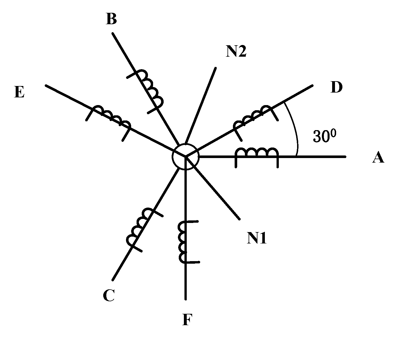
5]. The six-phase motor has attracted more and more attention because of its close connection with the traditional three-phase motor. The asymmetric dual three-phase permanent magnet synchronous motor has greater advantages because of smaller torque ripples [
5,
6]. It has two sets of three-phase windings with isolated neutral points, which are spatially shifted by 30 degrees, as shown in
Figure 1.
The vector space decomposition (VSD) method is widely adopted for the control of an asymmetric dual three-phase permanent magnet synchronous motor (ADT-PMSM) [
7,
8]. According to the dimensions of current control, the control methods based on the VSD can be divided into two kinds: two-dimension current control [
9,
10] and four-dimension current control [
11,
12,
13]. Two-dimension current control only establishes the current closed-loop control strategy in the
α-ß subspace where electromechanical energy conversion takes place, while an open-loop control strategy is adopted in the
x-y subspace. The fifth and seventh harmonic voltages due to the dead time effects of inverter will cause large harmonic currents. So, the two-dimension current control cannot achieve the desired results, while the four-dimension current control can control the currents of two subspaces separately. A current closed-loop control strategy is set up in the
x-y subspace to make the harmonic currents 0, which can compensate for the dead-time effects and the nonlinearities of the inverter [
13].
In References [
14,
15], by suitably selecting the voltage vectors from the divided vector groups into one sampling period, the current harmonics can be reduced compared to the Switching Table based Direct Torque Control (ST-DTC) drive. However, this method can only avoid injecting harmonic voltages into the
x-y subspace. However, the dead time and nonlinearities of the inverter are not considered. Methods based on a proportional–integral (PI) controller due to its simple structure and well-known characteristics are employed in the
x-y subspace. However, the fifth and seventh current harmonics are only suppressed to some extent due to its limited bandwidth [
16]. Accordingly, a multiple synchronous frame (MSF) scheme based on a PI controller in several synchronous frames (SF) in parallel (one per harmonic) is employed to eliminate the current harmonics in multi-phase machines, which can attain zero steady-state error at different harmonics. However, the computational burden is heavy. In [
13,
16,
17], a resonant controller is employed in an anti-synchronous frame rotating with the negative sequence fundamental frequency in the
x-y subspace to suppress the current harmonics, but the discretization errors of the poles are not considered.
In the field of current harmonics suppression of three-phase motor drives, extensive research has been conducted. Methods based on voltage-second balance theory classify the causes that distort the voltages. By offline measurement of the dead time, the turn-on/off time, and the nonlinearities including the forward voltage drop of the switching device and voltage drop of freewheeling diode, the compensation voltages can be calculated [
18,
19,
20]. However, these parameters are varied with the junction temperature of the inverter, motor load, speed, and some other factors. Accordingly, online methods are proposed in [
21], but these methods add computational burden to the algorithm and require a lookup table to search for the corresponding parameters under certain operating points. Besides, these above-mentioned schemes need the accurate polarities of phase currents [
18,
19,
20,
21]. Most methods detect the current polarities with current sensors, which are easily polluted by the noises and harmonics. In Reference [
22], a specific hardware circuit is designed to detect which antiparallel diode conducts in a one switching cycle to judge the current polarity. However, it adds burden to design the hardware. Similar to the current harmonics suppression of the ADT-PMSM, the resonant controller or the PI controller in the synchronous frames is also adopted [
23,
24,
25,
26]. Another approach that utilizes the integral term of the d-axis current as feedback to obtain the voltage distortion can only be used on condition that the d-axis reference current is a constant value [
27]. Some methods adopt a disturbance observer to estimate the voltage error, which does not need current polarities and the specifications of the inverter [
28,
29,
30,
31]. However, these methods require lots of efforts to obtain the observer gains and need to have a good knowledge of the motor parameters.
This paper proposes a method that combines the feedforward voltage compensation and the feedback voltage compensation methods together to suppress the current harmonics. The feedforward voltage compensation is obtained by the voltage-second balance theory, and the current detection scheme is independent of current sensors. In order to overcome the problems caused by the junction temperature and some other factors of the inverter, a feedback voltage compensation that employs a resonant controller is put forward. The proposed scheme can achieve the desired results without additional hardware or a good knowledge of the load parameters. The effectiveness of the proposed method is verified by a set of experimental results.
This paper is structured as follows:
Section 2 describes the mathematical model of ADT-PMSM. The analysis of dead-time effects is given in
Section 3. The feedforward voltage compensation and feedback current regulator designed in
x-y subspace are discussed in
Section 4.
Section 5 gives the pulse width modulation (PWM) techniques to implement the four-dimension current control of ADT-PMSM. Experimental results are carried out on an ADT-PMSM experimental platform to verify the effectiveness of the proposed method in
Section 6. Finally, the conclusions are summarized in
Section 7.
2. Machine Model of Asymmetric Dual Three-phase Permanent Magnet Synchronous Motor (ADT-PMSM)
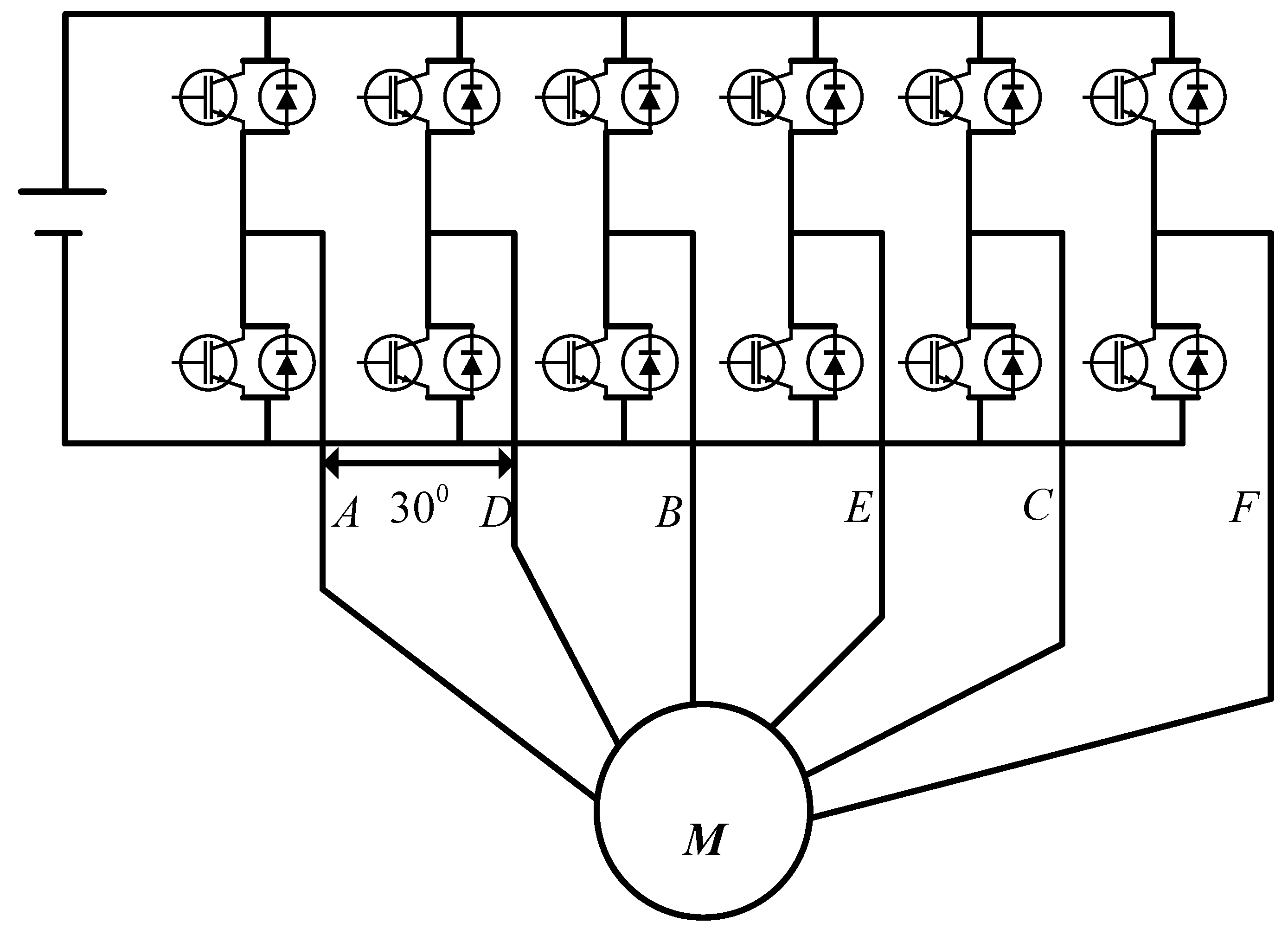
As depicted in
Figure 2, the drive system of ADT_PMSM in this paper has two sets of three-phase voltage source inverters (VSI) sharing the same DC-link voltage, which can supply two sets of three-phase windings.
According to the VSD theory, the variables including the current, flux, and voltage of the machine can be mapped into three orthogonal subspaces, i.e., the
α–β,
x–y, and zero-sequence subspaces. This approach gives an alternative description of the machine, which is useful for machine control and the development of pulse width modulation (PWM) techniques. Harmonics of different orders are mapped into different subspaces. The fundamental component and harmonics with the order 12n ± 1(n = 1, 2, 3 ...) are mapped into the
α–β subspace. The harmonics with the order 6n ± 1(n = 1, 3, 5 ...) are mapped into the
x–y subspace. The harmonics with the order 6n ± 3(n = 1, 3, 5 ...) are mapped into the
O1-O2 subspace, which is also called the zero sequence subspace. With neutral points being isolated, no current components in the
O1-O2 subspace would exist. Therefore, the ADT-PMSM with isolated neutrals is a four-order system. The mathematical model and the VSD modeling process of the dual three-phase motor in more detail are introduced in Reference [
9]. According to the magnitude invariant principle, the static decoupling transformation matrix is employed as
In order to achieve the vector control, a transformation is used to transform the
α–β variables into a synchronous reference frame rotating with the fundamental frequency, i.e.
where
θ is the electrical rotor position.
On the condition that the back electromotive force (EMF) is sinusoidal, two sets of windings are symmetric, and mutual leakage inductances are ignored. The voltage equations in the synchronous rotating
d-q coordinate axis in the
α–β subspace and in the stationary
x-y coordinate axis in the
x-y subspace are
where
R is the stator resistance,
Ld and
Ld are the
d- and
q-axes inductances respectively,
Lz is the leakage inductance, and
uk(
k =
d,
q,
x and
y) and
ik(
k =
d,
q,
x and
y) are the voltage and current components, respectively.
we is the electrical angular speed, and
ψf is the permanent magnet flux.
3. Analysis of Dead-Time Effects
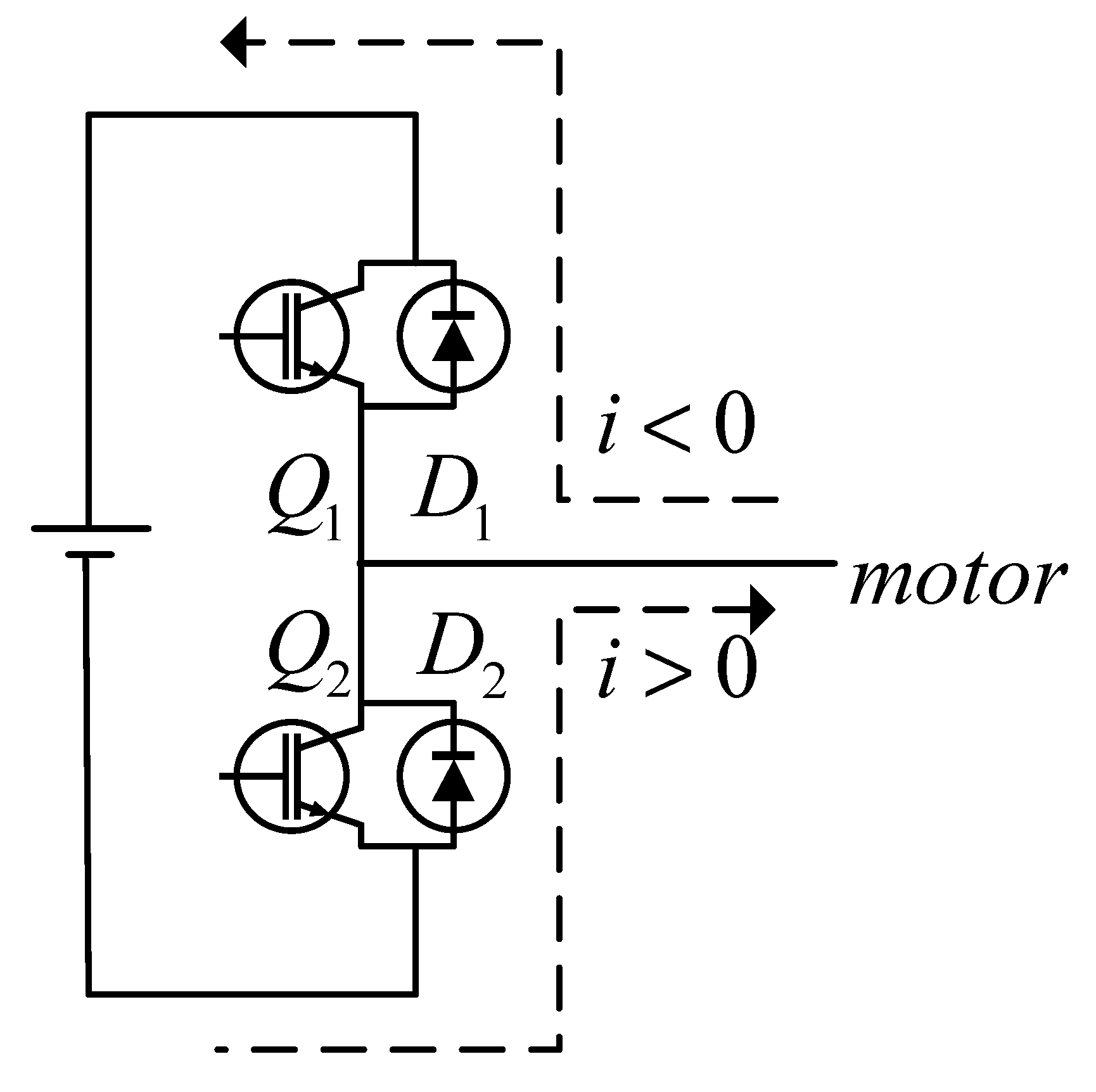
In order to facilitate the analysis,
Figure 3 shows one phase leg of the widely used six-phase PWM inverter during the dead-time period. If the phase current flows into the stator, the direction is defined as positive and vice versa.
In
Figure 3, the turn-on time is usually shorter than the turn-off time. In order to avoid the simultaneous conduction of both switching devices Q1 and Q2, fixed dead-time insertion is necessary to ensure the safety of the inverter system. The dead time could cause the desired reference voltages to distort and affect the control performance. During the dead-time period, both switches are turned off, and the current can only flow through the free-wheeling diode D1/D2, if the polarity of phase current is negative/positive. So, the output voltage relies on the direction of phase current during the dead-time period from the above analysis.
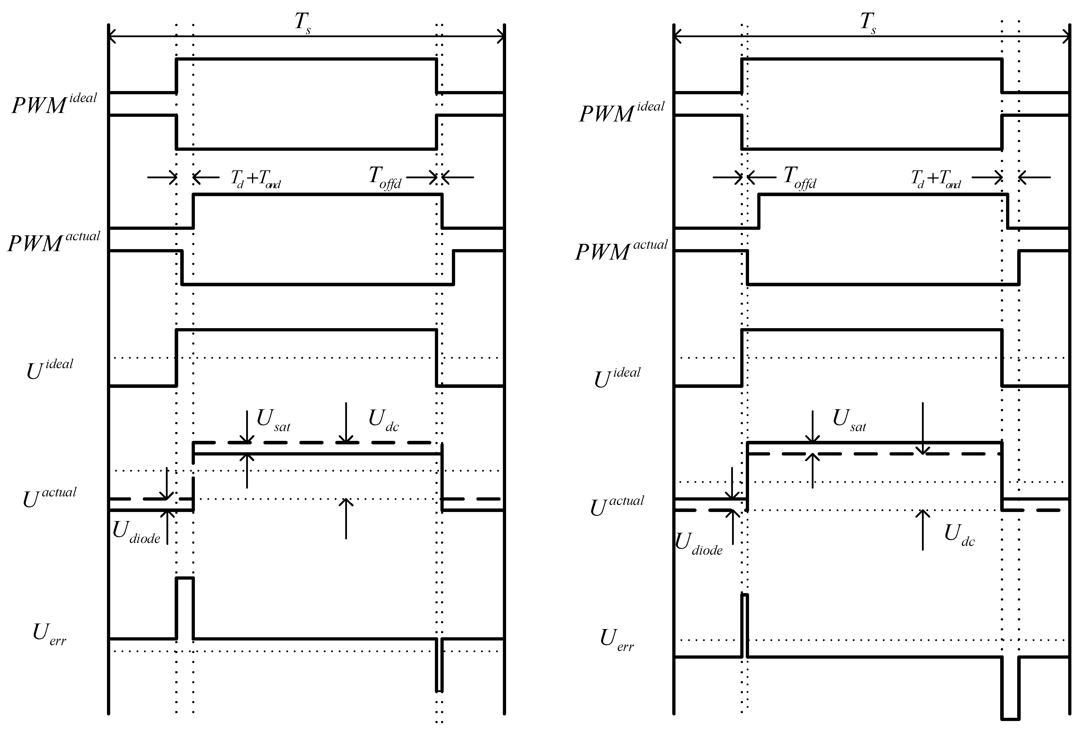
Taking the PWM waveforms of one phase leg for example,
Figure 4a,b show the situations when the phase current is positive or negative, respectively.
The average voltage error in one PWM period can be obtained as
where
sign(x) is a sign function and
Ud represents the magnitude of voltage error.
Ud can be expressed as
where
Td is the dead time,
Ts is the PWM carrier period,
Ton and
Toff are the on-period and off-period of the switching device of the inverter leg, while
Tond and
Toffd define the turn-on time delay and turn-off time delay of the switching device, respectively.
Usat and
Udiode denote the forward voltage drop of the switching device and the diode.
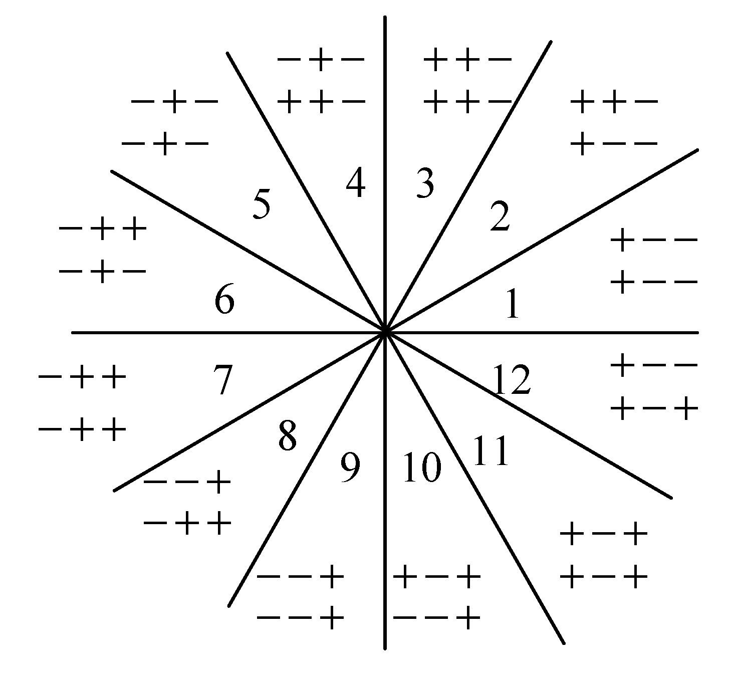
Uv represents the average voltage drop in one PWM cycle. The error voltages of six phases can be transformed into the
x-y coordinate axis in the
x-y subspace as follows:
where
Uxd and
Uyd are the error voltages in the
x-y coordinate axis in the
x-y subspace, while
UAd,
UBd,
UCd,
UDd,
UEd, and
UFd are the error voltages of phase A, B, C, D, E, and F, respectively.
The error voltages in the
x-y subspace can be obtained by applying the Fourier series as follows:
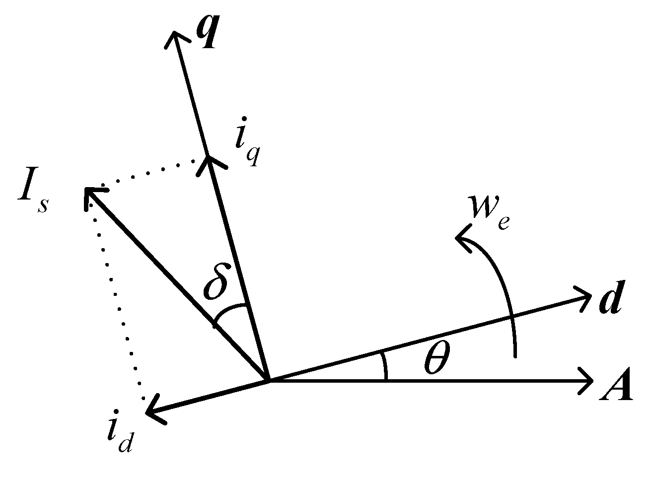
where δ denotes the angle between the current vector
Is and the
q-axis, as depicted in
Figure 5. Here, the anticlockwise rotation is defined as the positive direction. It is noteworthy that the fifth and seventh current harmonics will appear as the +5th and −7th in the
x-y coordinate axis in the
x-y subspace.
Applying the inverse Park transformation, the error voltages in the anti-synchronous rotating coordinate axis with the negative angular frequency
+we, which is defined as the
x1-y1 coordinate axis, become
where
Uxdx1 and
Uydy1 are the error voltages in the
x1- and
y1- axes respectively.
After the transformation, it is obvious that the sixth-order voltage components are the main contents of the error voltages. It will influence the motor currents, which will in turn affect the control performance. Assuming that the motor back EMF contains only the fundamental frequency, the sixth-order current harmonics in the virtual anti-synchronous rotating
x1-y1 coordinate axis in
x-y subspace are
where
.
It can be seen that the sixth-order current harmonics are dependent upon the speed and the parameters of the motor.
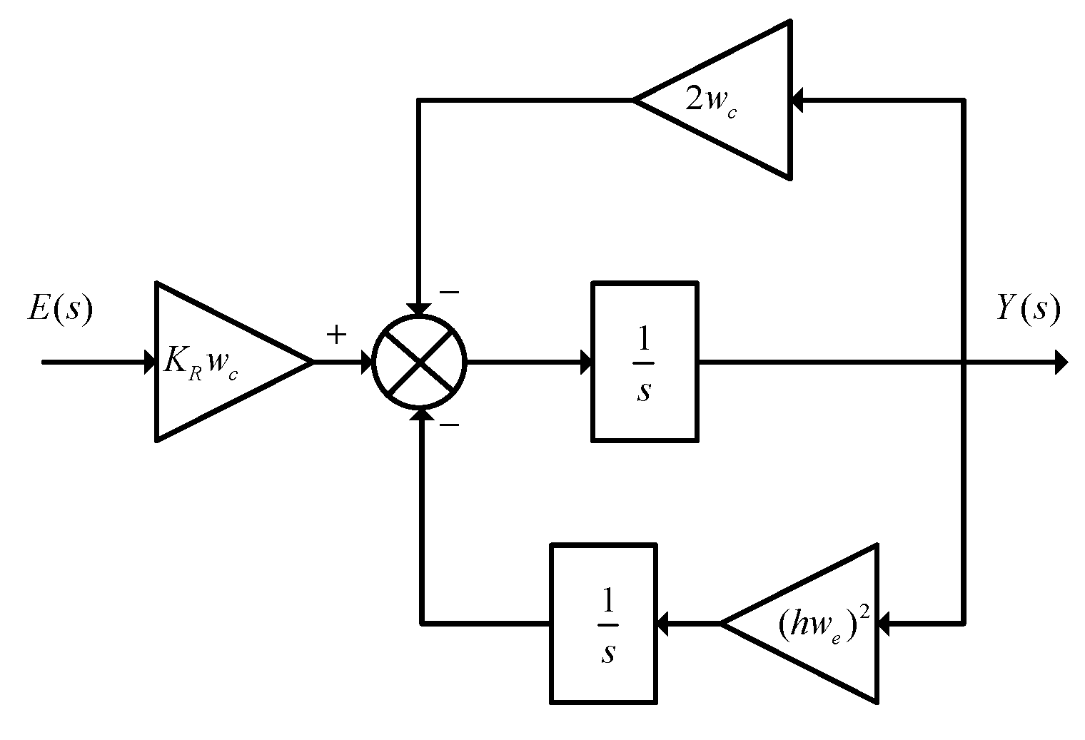
5. Pulse Width Modulation (PWM) Techniques for the Implementation of Four-Dimensional Current Control
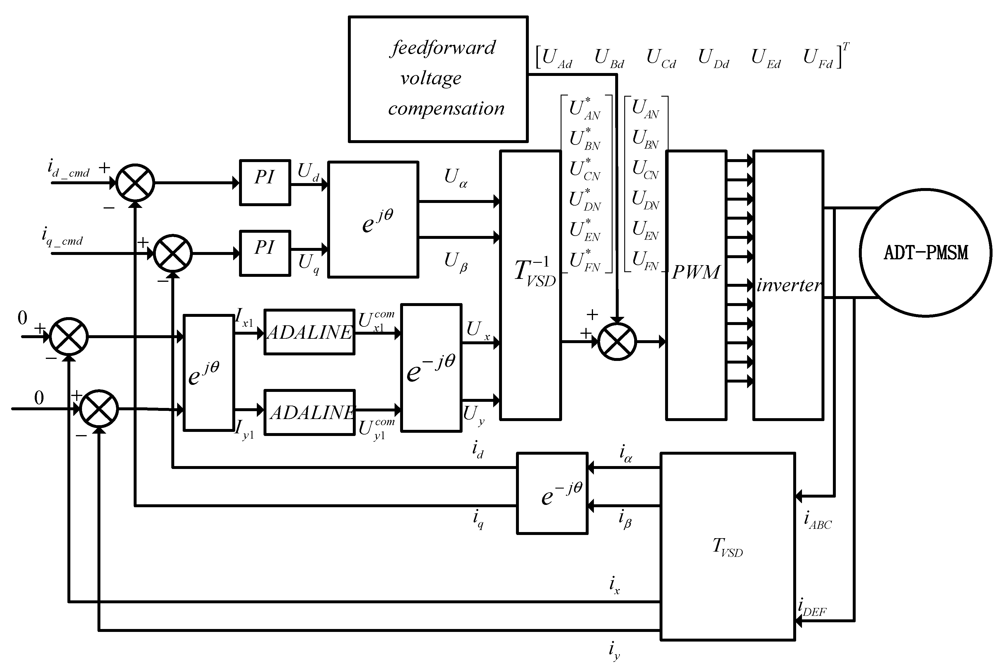
The block diagram of four-dimensional current control based on the VSD approach is illustrated in
Figure 10, which can compensate for nonlinear factors such as dead-time effects. After the feedback current control loop is adopted in both
α-ß and
x-y subspaces, the desired voltages
uα,
uß,
ux, and
uy can be acquired. Applying the inverse VSD transformation, the phase voltages after the feedback current control loop can be obtained as follows:
Adding the feedforward voltage compensations to the phase voltages obtained from Equation (20), the desired reference phase voltage vector is
where
UAd,
UBd,
UCd,
UDd,
UEd, and
UFd are the feedforward voltage compensations of phases A, B, C, D, E, and F, respectively.
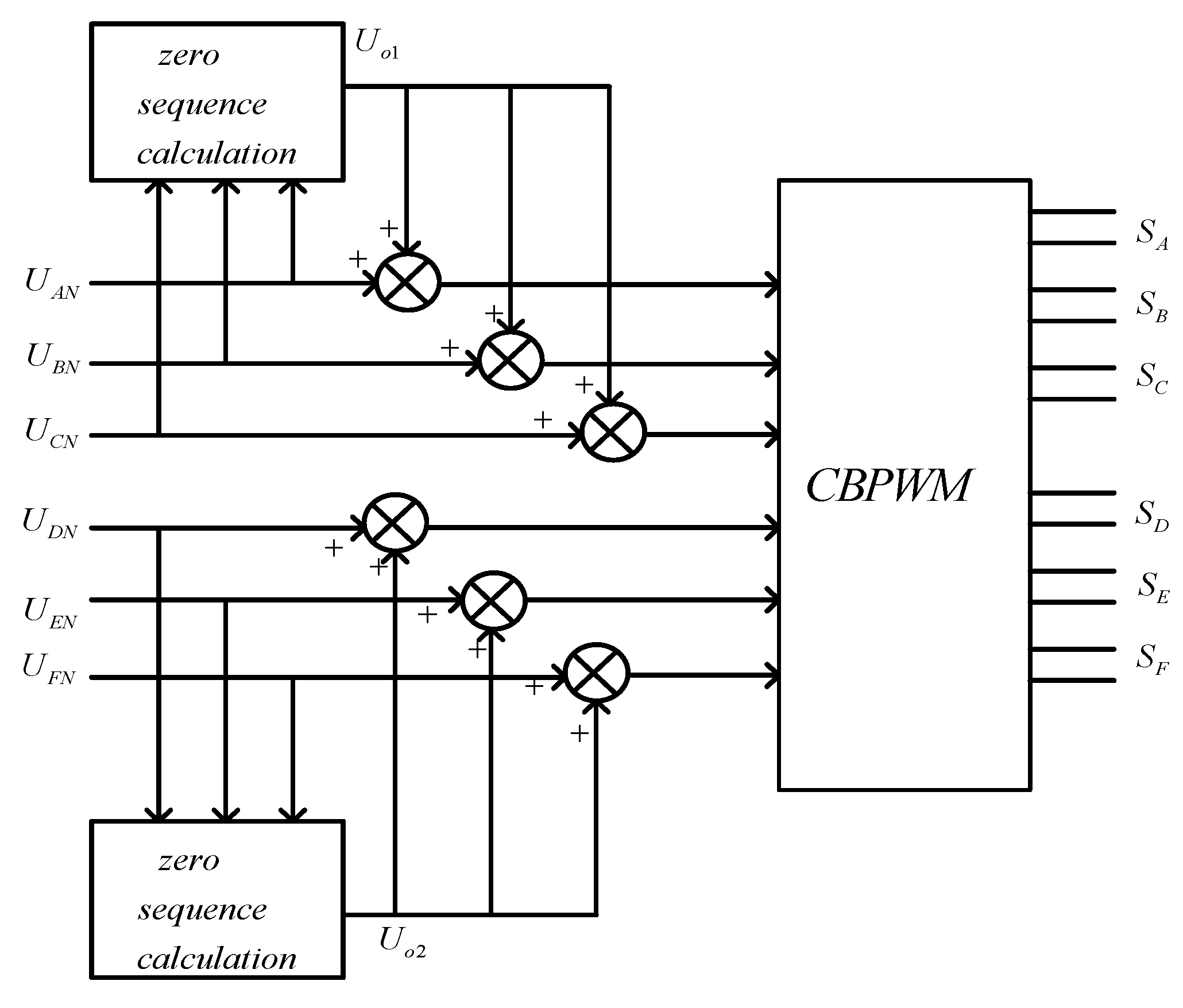
Due to the isolated neutral points of ADT-PMSM, the three-phase zero-sequence voltage injection PWM technique can be adopted. The output PWM waveform is modulated by comparing the final reference voltage waveform of each phase with the triangular carrier waveform, which is also known as the carrier-based pulse width modulation (CBPWM). There are many methods for calculating zero-sequence components. Different zero-sequence components are corresponding to different PWM strategies [
32]. In this paper, the commonly used mean zero sequence component injection, i.e., half of the middle value of the three-phase voltage values is used, as shown in Equation (22).
where
Umax,
Umid and
Umin are the maximum, middle, and the minimum values of the three-phase voltages.
Since the sum of three-phase voltages is zero, the zero-sequence voltage is equal to the half of the middle value of three-phase voltage values. It has been proved that the zero sequence voltage injection method is equivalent to the space vector pulse width modulation (SVPWM) algorithm, which can achieve the same linear voltage modulation range as proved in [
14,
15,
32]. Compared to the four vector SVPWM algorithm, a four-dimension current control for ADT-PMSM can be implemented. Besides, it is easy to implement and the PWM waveform is centrally symmetrical and each power device is switched only once in each PWM cycle. Besides, it will not introduce even harmonics and can reduce switching losses.
Figure 11 shows the double zero-sequence injection pulse width modulation (PWM) strategy.
6. Experimental Verification
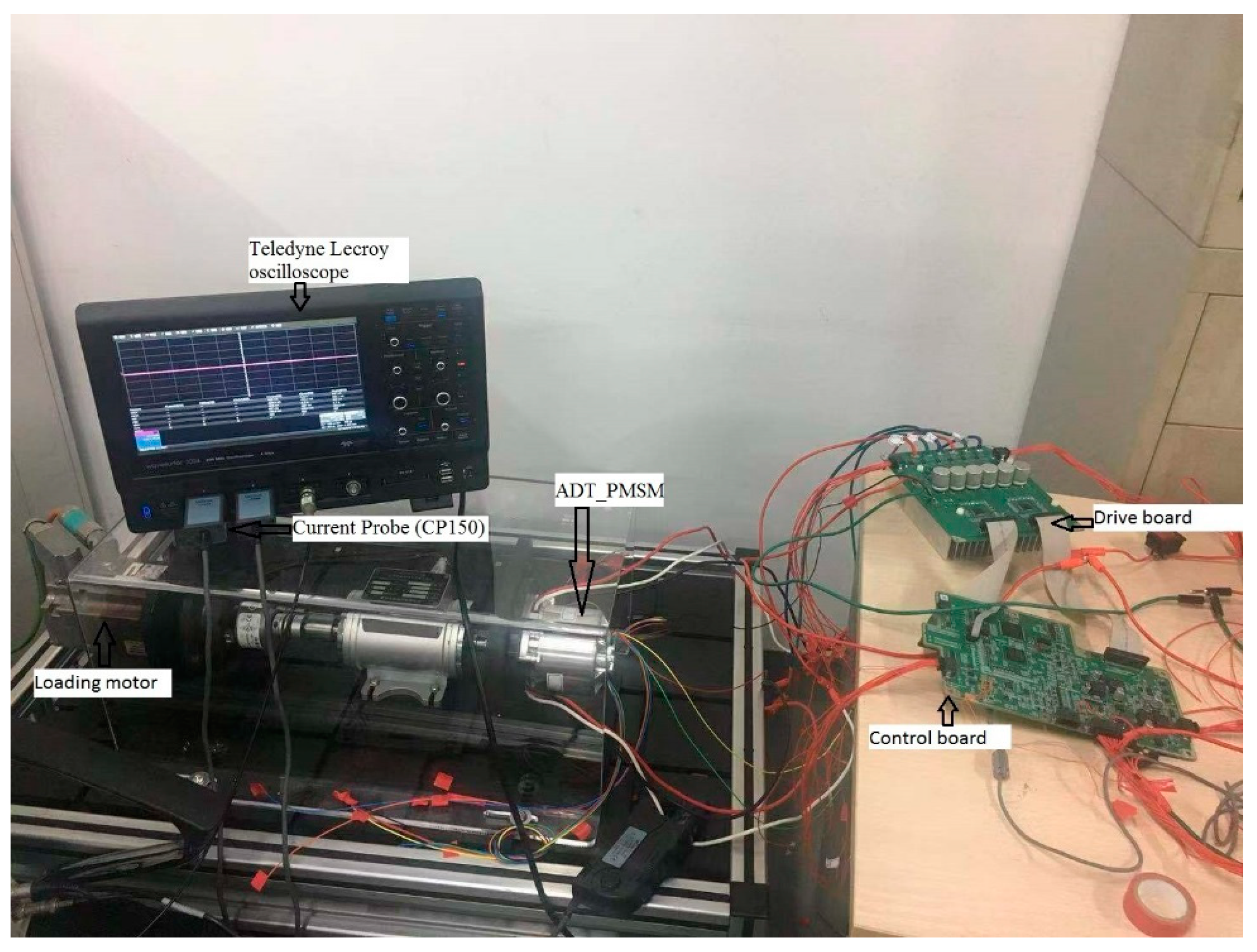
The effectiveness of the proposed current harmonic suppression algorithm is verified by the implementation in an ADT-PMSM experimental platform (Siemens, Munich, Germany). The experimental setup is shown in
Figure 12, which is composed of a DC machine mechanically coupled to the ADT-PMSM acting as a loading motor. The loading motor is controlled in speed control mode. The ADT-PMSM is supplied by using a two-level VSI (Infineon, Munich, Germany) configured for six-phase operation. A DC power supply is used to provide the DC-link voltage of 12V to the VSI. The complete control algorithm is implemented in a control board using Infineon TC277 (Infineon, Munich, Germany, 2017). The switching frequency is 10 kHz with 1
μs of dead time provided by the hardware in the VSI (Infineon, Munich, Germany, 2017). To provide the current display at higher resolution, a current probe (CP150, Lecroy, New York, America, 2013) and Teledyne Lecroy oscilloscope (WaveSurfer 3024, Lecroy, New York, America, 2016) are used. The data of the phase currents are saved as Excel files with the help of an oscilloscope.
The parameters for ADT-PMSM are given in
Table 1, and the specifications of VSI are given in
Table 2.
Four cases are listed below to compare the performances.
Case 1: The algorithm is implemented without feedforward voltage compensation and a resonant controller;
Case 2: The algorithm is implemented with feedforward voltage compensation only;
Case 3: The algorithm is implemented with resonant controller only;
Case 4: The algorithm is implemented with both feedforward voltage compensation and a resonant controller.
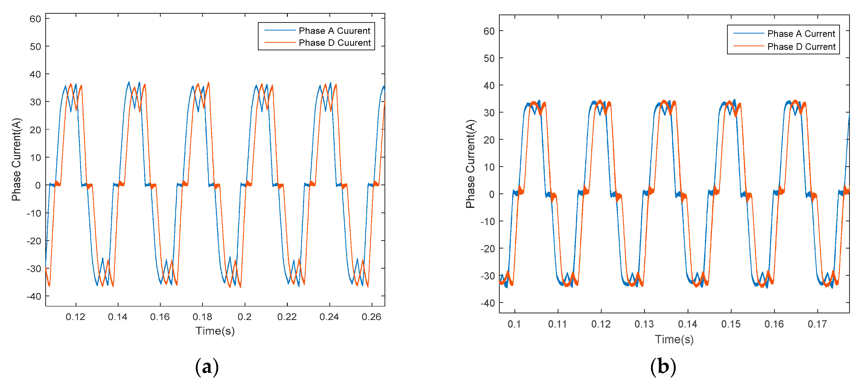
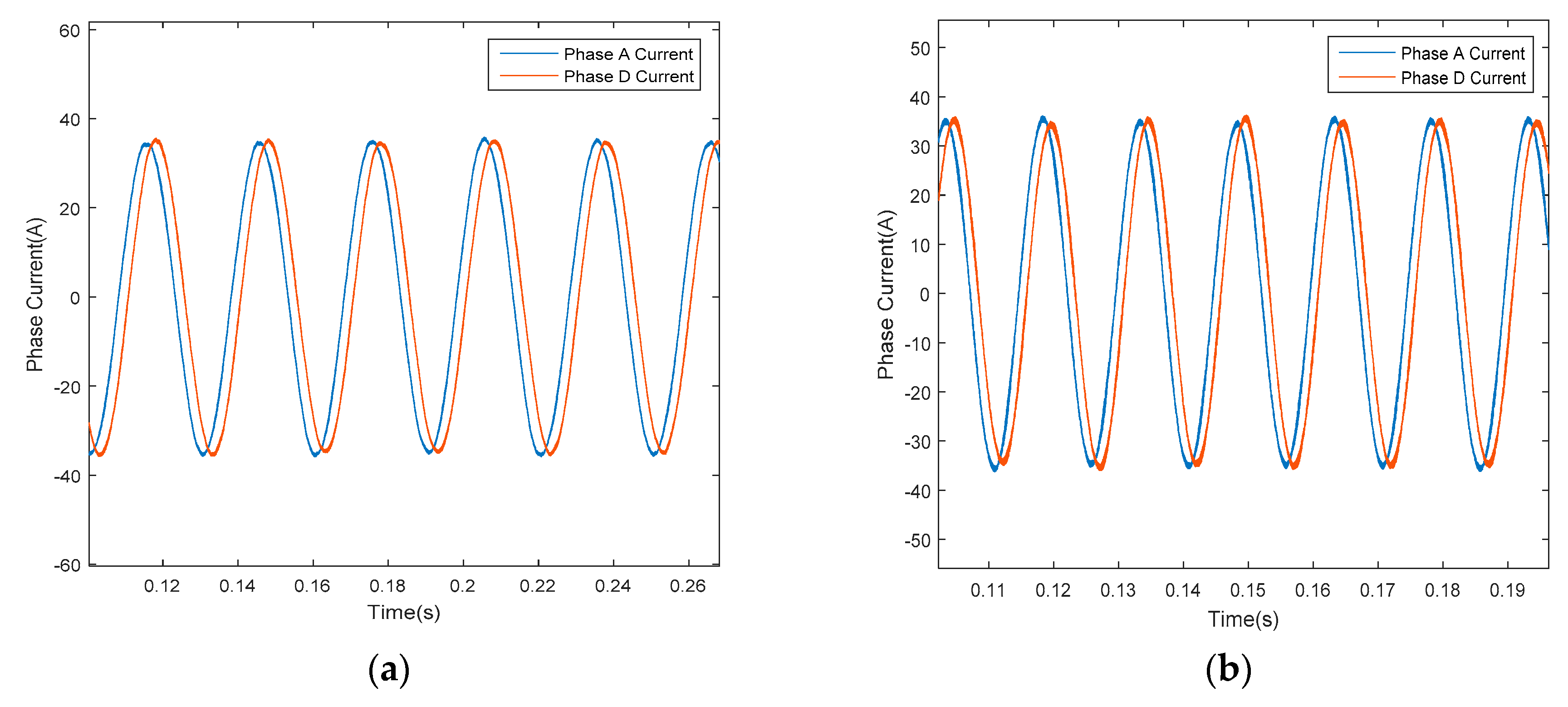
Figure 13 shows the experimental results without employing feedforward voltage compensation and a resonant controller, which is equivalent to Case 1. Here, the command currents
id and
iq are set to be 0 A and 35 A, respectively. The ADT-PMSM is operating under a current control loop and the speed is maintained at 500 rpm and 1000 rpm by the loading motor, respectively. Without the current closed-loop control strategy in the
x-y subspace and feedforward voltage compensation method,
ux and
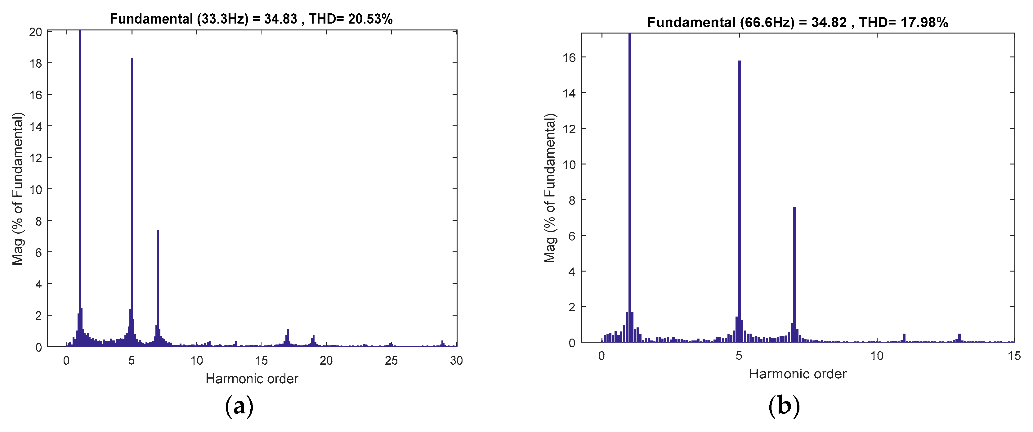
uy are set to be 0 in order to avoid injecting extra harmonic voltages. It is obvious that the phase currents are severely distorted due to the dead-time effects and some other factors. A fast Fourier transform is conducted on the phase A current waveform as illustrated in
Figure 14. From the figure, one can see that the phase current contains dominant fifth and seventh current harmonics and the total harmonic distortions (THD) are 20.53% and 17.98% respectively. Besides, it can be seen that the system is more sensitively influenced by the error voltage at low speed than at high speed, because the voltage error caused by dead time accounts for a large proportion at low speed.
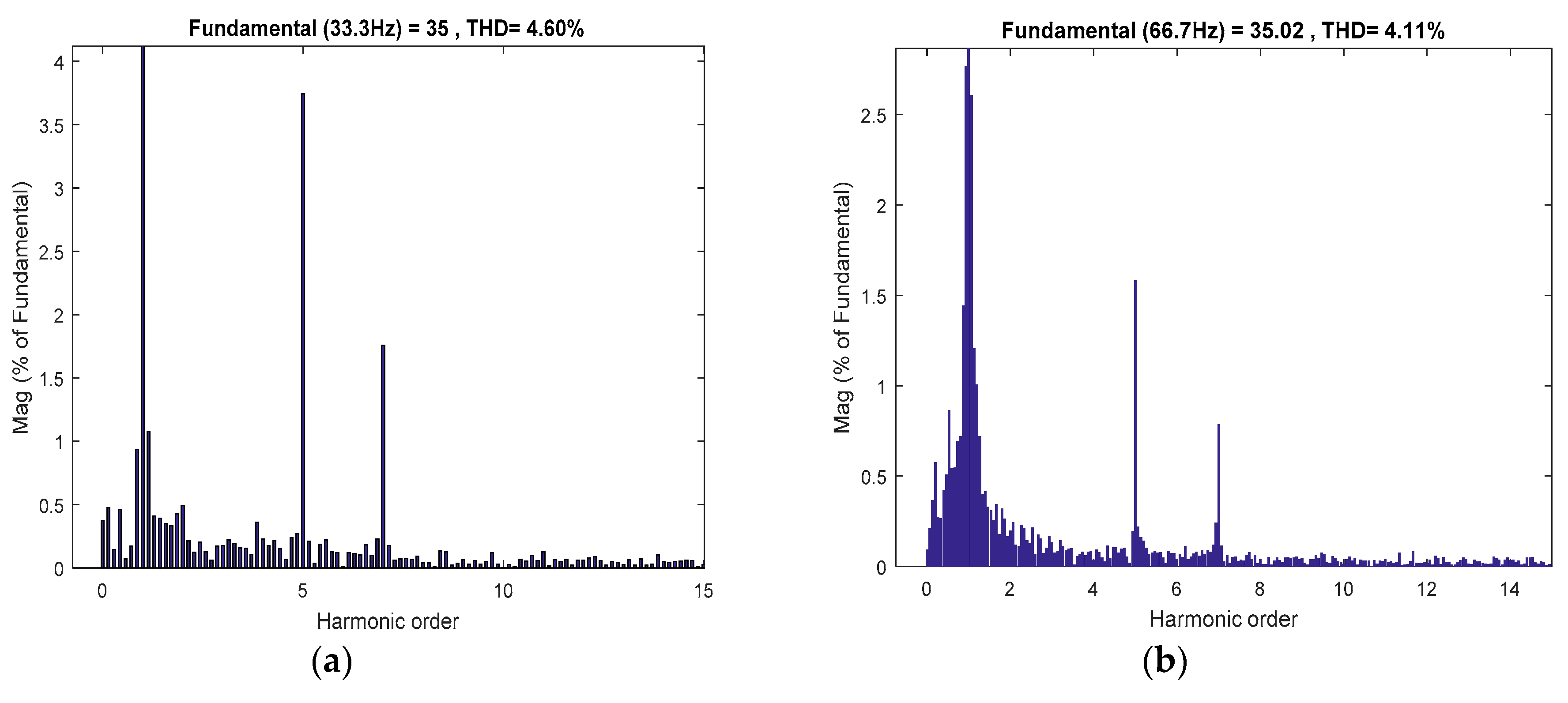
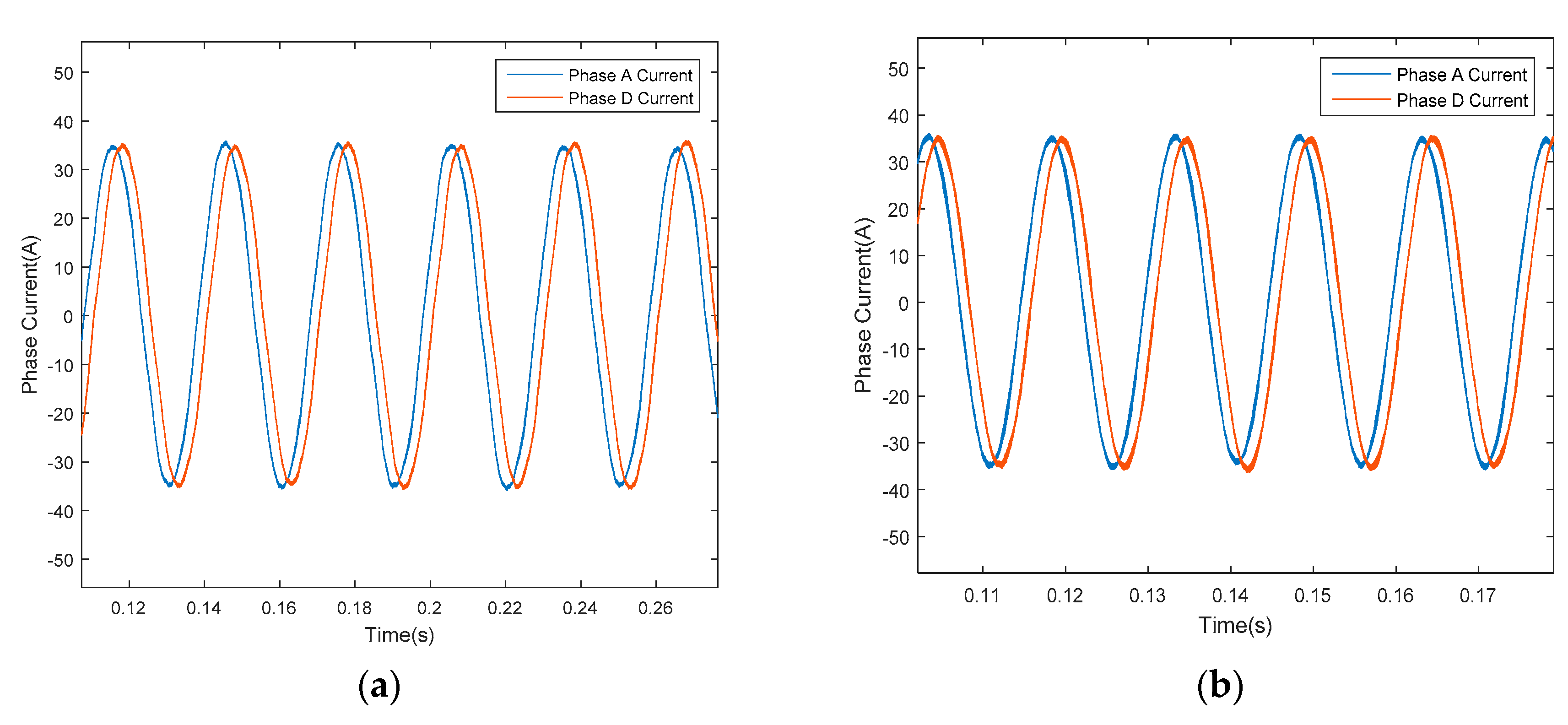
Figure 15 depicts the experimental results after adopting the proposed feedforward voltage compensation which is equivalent to Case 2. The compensating voltages are calculated based on Equations (4), (5), and (6). The reference voltages are synthesized based on the proposed SVPWM method illustrated in
Section 5. The waveforms of the phase currents have been improved a lot. The fifth and seventh current harmonics are significantly reduced. The THDs of the phase A current are reduced to 4.60% and 4.11% respectively with the proposed feedforward voltage compensation method, as shown in
Figure 16.
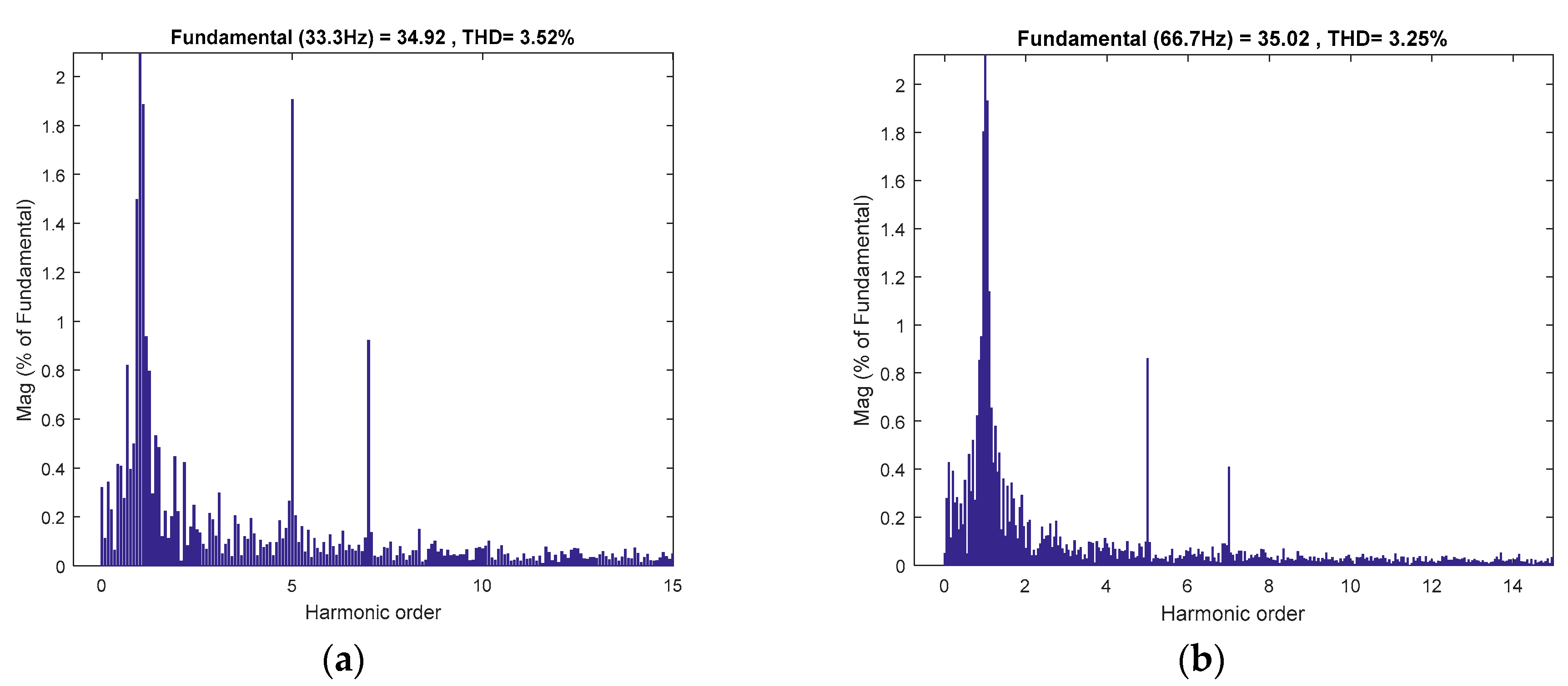
Figure 17 shows the experimental results after adopting the proposed resonant controller, which is equivalent to Case 3. The reference voltages are synthesized based on the proposed SVPWM method, as illustrated in
Section 5. The waveforms of phase currents have been improved. The fifth and seventh current harmonics are significantly reduced. The THDs of the phase A current value are reduced to 3.52% and 3.25% respectively with the proposed resonant controller, as shown in
Figure 18.
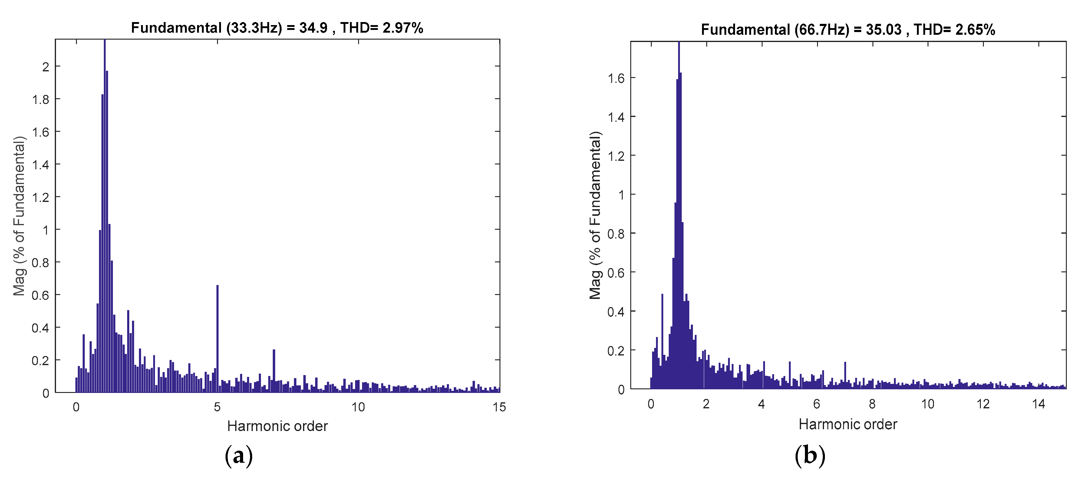
Figure 19 depicts the experimental results after adopting both the proposed feedforward voltage compensation and resonant controller, which is equivalent to Case 4. The reference voltages are synthesized based on the proposed SVPWM method illustrated in
Section 5. The waveforms of phase currents have been improved a lot, while the fifth and seventh current harmonics are significantly reduced. The THDs of the phase A current are reduced to 2.97% and 2.65% respectively with the proposed combination method, as shown in
Figure 20. The THDs are the smallest among the four above-mentioned cases.
In order to facilitate the analysis,
Table 3 shows the comparison of the THDs for four different cases under 500 rpm where the phase currents are 20 A and 35 A, respectively. The switching frequency is 10 kHz with 1
μs of dead time. It can be seen that the THD when the phase current is 35 A is smaller than the THD when the phase current is 20 A, because the fundamental component is smaller when the phase current is 20 A. Besides, it is apparent that although the methods adopted for Case 2 and Case 3 can suppress the current harmonics effectively, the scheme for Case 4 is even more superior to the methods adopted for Case 2 and Case 3.
Table 4 depicts the comparison of THD values for four different cases under 1000 rpm and phase currents are 20 A and 35 A, respectively. The switching frequency is 10 kHz with 1
μs of dead time. It can be seen that as the speed increases, the system is more sensitively influenced by the error voltage at low speed than at high speed, because the voltage error caused by dead time accounts for a large proportion at low speed. We can obtain the conclusion that feedforward voltage compensation and the feedback current control loop in the
x-y subspace can suppress the current harmonics effectively, and employing both methods at the same time can achieve even better results.


