Abstract
Researchers frequently use visualizations such as scatter plots when trying to understand how random variables are related to each other, because a single image represents numerous pieces of information. Dependency measures have been widely used to automatically detect dependencies, but these measures only take into account a few types of data, such as the strength and direction of the dependency. Based on advances in the applications of deep learning to vision, we believe that convolutional neural networks (CNNs) can come to understand dependencies by analyzing visualizations, as humans do. In this paper, we propose a method that uses CNNs to extract dependency representations from 2D histograms. We carried out three sorts of experiments and found that CNNs can learn from visual representations. In the first experiment, we used a synthetic dataset to show that CNNs can perfectly classify eight types of dependency. Then, we showed that CNNs can predict correlations based on 2D histograms of real datasets and visualize the learned dependency representation space. Finally, we applied our method and demonstrated that it performs better than the AutoLearn feature generation algorithm in terms of average classification accuracy, while generating half as many features.
1. Introduction
Understanding the statistical relationships between random variables (or features) is a fundamental problem in the fields of statistics and machine learning. Researchers usually visualize the features of a dataset (e.g., using scatter plots) to understand the dependencies between variables. For example, in supervised learning, researchers use visualizations of the features to understand which features are relevant or irrelevant to the values of the target variables, and how the relevant features are related to the target variables. They then select learning algorithms based on the dependence types. However, if the number of features is large, interpretation of visualizations is cumbersome and time-consuming.
Therefore, many dependence measures have been developed to automatically detect dependency relationships. A number of information-theoretic measures have been invented based on the Shannon entropy [1]. Mutual information (MI) [2] and its variants have been widely used to analyze categorical or discrete features [3]. Various types of correlations have been developed to help categorize the relationships between continuous features: Pearson’s correlation coefficient (pCor), Spearman’s rank, Kendall’s tau, distance correlation (dCor) [4], maximal information coefficient [5], the randomized dependence coefficient [6], and etc.
Various applications of dependency measures have been developed. Li et al. [7] used dCor to screen the features of gene expression data. Zeng et al. [8] proposed a variant of MI to measure interactions between features to aid feature selection. Chen et al. [9] applied MI to the representation learning of generative adversarial networks (GANs). Kaul et al. [10] presented an automated feature generation algorithm based on dCor called AutoLearn.
Existing dependency measures are subject to three main limitations. Firstly, they do not consider dependency types. For example, in Figure 1, the dCor of all feature pairs is 0.5, but the types of dependence are obviously different. Secondly, these measures are human-readable scalars rather than machine-readable vectors. Thirdly, they are not optimized to specific applications.
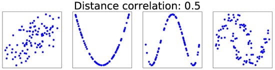
Figure 1.
Various dependence types with the same distance correlation of 0.5.
These three problems can be solved by using visualizations as inputs to convolutional neural networks (CNNs). Firstly, dependency types can easily be classified based on visualizations, as shown in Figure 1. The visualizations, such as scatter plots, can be regarded as images. Advances in deep learning-based computer vision have proven CNNs to be effective for processing high-dimensional images. CNNs are frequently used for image classification [11], object detection [12], and image generation [13]. Secondly, neural networks are also capable of learning machine-readable representations; for example, word representations [14] from textual data have achieved great success in natural language processing [15]. Likewise, dependence representations can be learned by CNNs if an appropriate learning method is applied. Thirdly, when applying an end-to-end (feature learning) approach, CNNs can learn task-specific representations from visualizations, and thus they can be optimized for a specific task (such as text recognition [16], speech recognition [17], and self-driving cars [18]) based on dependency measures. Basically, the usage of CNNs is motivated by the fact that they can extract significant features from visualizations at different hierarchical levels.
Thanks to the above advantages of CNNs, the hand-crafted representations may be replaced with convolutions. A few previous studies used deep neural networks (DNNs) for dependence estimation; for example, Belghazi el al. [19] used DNNs for estimation of mutual information between high dimensional continuous random variables. Hjelm et al. [20] proposed an unsupervised learning method, called Deep InfoMax, for representation learning. Similarly to our work, they tried to perform dependence estimation for specific tasks, but used mutual information as estimation target and they focus only on high dimensional variables such as images. To measure statistical dependence, correlations have been widely used in the fields of statistics and machine learning. However, due to a large amount of types of nonlinear dependence, it is very challenging to distinguish the types with a correlation coefficient. When using CNNs for dependence learning, we should consider one of its important disadvantages; CNNs have a huge number of parameters and with small dataset, would run into an overfitting problem, and thus they require much more training data than other existing learning algorithms.
In this paper, we present a dependence representation learning algorithm in which CNNs extract task-specific dependence representations from visualizations of feature pairs. To the best of our knowledge, this is the first method that directly captures dependencies from visualizations of random variables. As the inputs of CNNs, we use 2D histograms, which are compressed scatter plots. In order to show that CNNs can learn dependence representations from 2D histograms, we have conducted three sorts of experiments: In the first experiment, we used a CNN to perfectly classify eight dependence types of a synthetic dataset. Next, we trained the CNN to simultaneously predict Pearson and distance correlations. Our results demonstrated that the CNN can predict the correlations well. Finally, we applied the dependence learning method and found that it outperformed the AutoLearn feature generation algorithm in terms of average classification accuracy and generated half as many features.
2. Dependence Representation Learning
2.1. Method
In this section, we define dependence representation learning, which allows neural networks to extract task-specific dependence representations from visualizations of feature pairs. The neural networks are trained in a supervised manner, but the targets for supervised learning can be generated without manual effort.
Given a feature pair , a visualization matrix V is computed by
where the function ‘visualize’ is a visualization method, such as a 2D histogram. Given a dataset of 2D array values, a 2D histogram shows the number of elements in each bin, by drawing colors of corresponding intensity. In image processing, a 2D histogram shows the relationship of intensities at any position between two images. In our work, the 2D histogram of two random features is used for training the CNNs to classify the dependence types and predict correlations.
is the feature plotted on the x-axis of the visualization, and is the y-axis. The dependence representation vector Z is extracted from the visualization V using a neural network with parameters :
We then compute the desired dependence target of the feature pair (e.g., dependence type, correlation, or usefulness of the pair):
where ‘’ is a function that outputs the target. Finally, the neural network is trained by minimizing the objective function defined as follows:
where is an activation function and w is a weight vector that maps representation Z onto target T. is a set of feature pairs, and is a loss function for a specific task, such as the cross entropy or mean squared error (MSE). The dependence representation learning algorithm is described in Algorithm 1.
| Algorithm 1 Dependence representation learning. | ||
| 1: | initialize network parameters | |
| 2: | repeat | |
| 3: | for do | // m: mini-batch size |
| 4: | Sample a feature pair from set of feature pairs | |
| 5: | ||
| 6: | ||
| 7: | end for | |
| 8: | Update the network and w by descending their stochastic gradients: | |
| 9: | until convergence of | |
2.2. Implementation
To keep the experiments simple, we implemented the visualization method and neural network in the same way each time. The specific implementations of the target and loss functions depend on the task. Figure 2 shows our implementation of dependence representation learning. As training data, feature pairs are transformed into 2D histograms and then input into CNNs. The CNNs are trained by minimizing the loss between the outputs and the targets computed from the feature pairs.
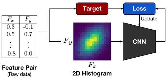
Figure 2.
The implementation of dependence representation learning.
The visualization method : scatter plots are frequently used to visualize dependencies between features. However, scatter plots are usually rendered as images that contain many individually specified pixels. Thus, if we use scatter plots as inputs to CNNs, then we will suffer from the curse of dimensionality. Therefore, we used density-based 2D histograms, which can be considered as compressed scatter plots. Another advantage of density-based histograms is that their representations are almost equivalent for different feature pairs, as long as the features come from the same distribution. However, histograms are often skewed by a small number of outliers. Thus, we remove outliers from each feature before converting the data into a histogram. A sample of a feature is an outlier if , where:
The MAD stands for median absolute deviation, which is defined by
The neural network : CNNs have been hugely successful in various computer vision applications. We use CNNs because we assume that they are the most advanced model for processing visual information. More specifically, we use the DenseNet architecture [21], which is a widely-known image classification model. Here, we used representation vectors with 1734 elements.
Common implementation details: again, for simplicity, we tried to apply a unified training method as much as possible in all experiments. The common implementation details for the rest of the paper are as follows, though some task-specific details are described in later sections for each task. We use PyTorch [22] to train the CNNs, scikit-learn [23] for machine learning algorithms, and NumPy [24] to generate the 2D histograms and carry out numerical tasks. Here, the number of 2D histogram bins is 16, resulting in an input shape of . We trained CNNs using the ADAM optimizer [25] and a mini-batch size m of 64.
3. Case Studies
Before describing feature generation, we outline the results of two simple empirical evaluations. Note that our goal is to show that CNNs can learn dependence representations from 2D histogram input.
3.1. Dependence type Classification
As mentioned in the introduction, existing dependency measures cannot classify various types of dependency shown in Figure 3. In comparison, this experiment shows that our CNN-based proposed method can classify eight types of dependency almost perfectly.
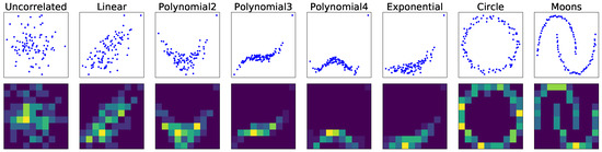
Figure 3.
Examples of the synthetic datasets used to classify the types of dependency. Top: Scatter plots of the synthetic feature pairs. Bottom: 2D histograms of the synthetic feature pairs.
3.1.1. Experimental Setup
To develop a trained CNN model for dependence type classification, we generate a set of feature pairs as a training data as seen in Figure 2. Firstly, except for the ‘Circle’ and ‘Moons’ dependency types, we have generated synthetic feature pairs by firstly generating by sampling from a standard normal distribution, then using to compute for the dependence type, including some noise. Secondly, we have generated the synthetic feature pairs for the ‘Circle’ and ‘Moons’ types. Such synthetic data ware generated on-the-fly, during training, and thus each training set was different. Consequently, we have generated a total of 6400 feature pairs with 800 feature pairs for each dependence type and trained the CNNs with a cross-entropy loss, a softmax output layer, and a learning rate of . To avoid overfitting, we used a weight decay of and added dropout layers [26] with a ratio of 0.2 after each convolutional layer, as outlined in [21].
3.1.2. Results
Quantitative results. Figure 4 shows the results obtained with the training and test sets: (a) the cross-entropy loss and (b) the classification accuracy of the CNN on the training and test sets. The loss and accuracy values are recorded every 100 iterations. The test accuracy of the CNN reached 100% after only 600 iterations (or updates) even though there was a slight performance degradation at 800 iterations. More importantly, there was no sign of overfitting since the training loss was always higher than the test loss, as shown in Figure 4a.
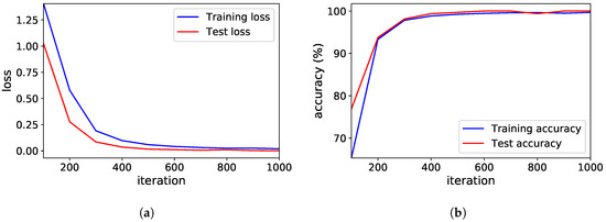
Figure 4.
The results of the dependence type classification. (a) Loss, (b) accuracy.
Qualitative results. Figure 5 shows visualizations of the dependence representations for the test set. The 1743-dimensional dependence representations learned with dependence type classifications are reduced into 2-dimensional vectors using t-stochastic neighbor embedding (t-SNE) [27] and principal component analysis (PCA) [28], which are visualized on the 2-dimensional space of each subfigure, respectively. In order for the classification of dependence types to be accurate, the learned results of dependence representations should be clustered. As shown in the figure, the representations are perfectly clustered by their dependency type. In particular, in the right subfigure of PCA visualization, ‘Polynomial3’ and ‘Polynomial4’ types of representations are positioned closely because they look actually similar, even though they are of different types. We interpret this figure as indicating that the dependence representations can not only capture similar dependence types, but also classify them with slight differences.
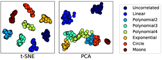
Figure 5.
Visualizations of dependence representations learned with dependence type classification.
3.2. Correlation Regression
The correlation regression is a task of learning the representation of dependencies with visualizations of two random features. We assume that a trained model is capable of extracting a particular representations if it can predict correlation coefficients between the features. The purpose of this experiment is to verify that visualization methods can express dependencies and that machine learning methods can learn representations from visualization inputs and predict correlation coefficients. Hence, in this experiment, we have investigated whether the CNNs are capable of estimating correlations based on 2D histograms of real data, and thus we have found that inputting histograms into CNNs is sufficient for reproducing existing domain knowledge about dependence, namely the correlations.
3.2.1. Background: Correlations
Pearson’s correlation (pCor): pCor is the best known and most widely used correlation metric. It measures linear dependence and has a range of , where is a perfect positive linear correlation and is a perfect negative linear correlation. A pCor of zero means that the features are not linearly correlated, but does not mean that the variables are independent. Note that pCor cannot capture any type of nonlinear dependence.
Distance correlation (dCor): in contrast to pCor, dCor can be used to analyze nonlinear relationships, but cannot measure the direction of the correlation. The dCor takes values between and it is equal to zero if and only if the two random variables are independent. As dCor tends to 1, the linearity of the relationship increases. One disadvantage of dCor is its computational complexity, which is . A fast computation algorithm with complexity was proposed to overcome this disadvantage [29].
3.2.2. Method
We modified Equation (1) to train CNNs to predict dCor and pCor based on 2D histograms. We define individual objective functions for dCor and pCor, and then combine them. First, the objective function for dCor is defined by:
where is a sigmoid function, which has the same value range as dCor, and is a function that returns the dCor of the features. Second, we define the objective function for pCor by:
where is a function that returns pCor of the features. We used as an activation function that matches the value range of pCor. Finally, we defined the objective function for the correlation regression by combining the two functions defined above:
Because the range of pCor is double that of dCor, we balance the two losses by halving . Note that the representation Z is used to predict both dCor and pCor. We optimized the neural net and the weight vectors w by minimizing the correlation regression loss :
where W is the set of all weight vectors. We evaluated these, then predicted dCor and pCor as:
and:
3.2.3. Experimental Setup
Datasets: in order to evaluate our proposed method for correlation regression, we have collected real-world datasets that contain various features. Table 1 describes the 172 real-world datasets used for the training and evaluation: 159 for training, and 13 for testing (see Table 4 for the detail of testing data). The datasets have been selected from OpenML [30] only for classification and we generated feature pairs for each dataset separately. Moreover, we have adopted only continuous features because correlations are not appropriate measures of categorical features.

Table 1.
Description of datasets used for correlation regression and feature generation.
Implementation details: like 2D histograms, correlations are also easily skewed by a small number of outliers. Hence, we applied the simple outlier removal method of Equation (2) before computing the correlations. The learning rate of the optimizer is . We did not add any weight decay or dropout layers because no overfitting was identified. The dCor values ware computed using the fast implementation of dCor [29]; we clipped the values at zero because the dCor values output by the fast implementation can be negative when they are close to zero.
3.2.4. Results
Quantitative results: Table 2 lists the evaluation scores of each correlation. The scores are reported in terms of the mean squared error (MSE), mean absolute error (MAE), and coefficient of determination (). In the cases of the MSE and MAE, lower values indicate better scores, but higher values are better in the case of; . For example, if we predict dCor based on a set of feature pairs that have a true dCor of 0.5, then based on the average MAE, the predicted value is approximately in the range of .
Table 2.
Correlation regression scores obtained for the test set.
Graphical analysis: we also analyzed the results graphically so that we could present them more intuitively and in more detail in Figure 6. Each point in the figure represents a single true-predicted correlation pair. The x-coordinate of a point represents the true correlation, and the y-coordinate is the correlation predicted by the CNN. The closer the points are clustered around the line , the better the performance. As seen in the figure, both sets of results are clustered around the line. One exception is in the case that the true value of dCor is equal to 0.0, when the predicted correlations are highly erroneous. This may be due to clipping the values at zero.
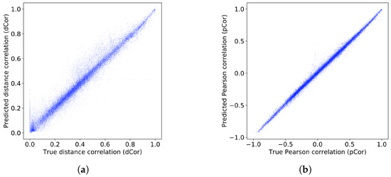
Figure 6.
Scatter plot of the true correlations against the predicted correlation on the test set: (a) dCor regression results; (b) pCor regression results. Note that the subfigures (a,b) have different ranges.
Qualitative results: Figure 7 depicts visualizations of the dependence representations learned via the correlation regression technique for the test set. As seen in the figure, the 1743-dimensional representations are reduced into 2-dimensional vectors using (a) t-SNE and (b) PCA in the same way as in Figure 5. Each of the learned representations is plotted as a dot on a 2-dimensional plane, and its corresponding true correlation values is indicated in color. Consequently, if the learned results are correct, then the dependence representations that are nearby in the representation space could produce color-coded clusters since they are displayed in the same, or similar color.
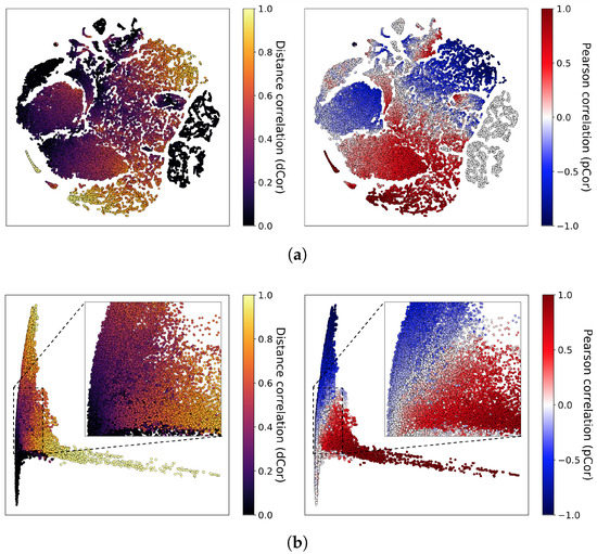
Figure 7.
Visualizations of the dependence representations of the test set. (a) t-stochastic neighbor embedding (t-SNE), (b) principal component analysis (PCA).
In each of the subfigures, the points to the left represent the true dCor value, and points to the right represent the true pCor value. Points that are close to gether have similar correlations. The independent feature pairs (dCor of zero) are clustered with themselves. The formation of coherent clusters of color as a whole indicates that the fundamental characteristics of given correlations have been well learned. Furthermore, the zoomed-in plots in Figure 7b show clusters of point that have a pCor of zero but a nonzero dCor.
R-unning time analysis: here, we need to consider another issue about running time; as earlier mentioned, the one major drawback of dCor is its high computational complexity. [29] proposed the algorithm, but it still takes a long time to compute when the sample size n is large. Table 3 provides a comprehensive comparison of the running times (in second) of methods for each sample size n. The running times of the fastest method are shown in bold face for each n. All the reported times ware measured using the same machine (Intel Xeon CPU E5-2698 v4 @ 2.20G Hz). We also compare the running time of our CNN-based method (denoted as CorrCNN) on CPU and GPU (GeForce GTX 1080Ti). The times reported for our method include times for creating a 2D histogram, transferring data to GPU, and running the CNNs.
Table 3.
Comparison of running times for distance correlation.
If dCor is implemented directly according to its definition [4], the running times are shorter than 1 s when in our experiments. In the case of the fast implementation of [29], the times are less than 1 sec when . Our method, however, only takes less than 1 s until n reaches on both of CPU and GPU. This is due to the fixed running time of our CNNs regardless of the sample size n, since the 2D histogram size is always equal no matter what the sample size is. The increasing time according to n results from running times for creating the 2D histogram. Note that our method is faster even on CPU when . According to the result, when a sample size is large, our method is more efficient than other methods.
4. Feature Generation
As an application of our dependence representation learning method, we have improved the AutoLearn feature generation algorithm [10], which generates new sets of features that are useful for classification tasks by combining pairs of features from the original ones based on some pre-defined operations; for example, basic arithmetic operations and correlation between two features can be constructed as new features. In this section, we summarize AutoLearn, describe our method, and report the results of our comparison between our method and AutoLearn.
4.1. Background: AutoLearn
4.1.1. Mechanism
The AutoLearn algorithm is composed of three steps:
- Preprocessing: shoose candidate features for feature generation by selecting features that are relevant to the classes of interest, as indicated by information gain (IG). If the number of features is less than 500, then use the features with an IG greater than zero; otherwise use the top 2% features.
- Feature generation: for all possible feature pairs of candidate features, generate new features by performing regression on input data are with target .
- Feature selection: select features that are useful for classification based on stability and IG.
4.1.2. Feature Generation Process
The novelty of AutoLearn is in step 2, where regression is applied to generate new features. The regression algorithm is selected based on the dependence types of the feature pairs. If they are linearly related, then linear ridge regression (LRR) [31] is used. If the dependency is non-linear, then kernel ridge regression (KRR) is used [32] with a radial basis function (RBF) kernel. The two types are categorized based on a threshold: if , then the data are linearly related; otherwise, they are non-linearly related. Note that there is no feature generation if the dCor of the feature pair is zero. Once the appropriate regression algorithm has been identified, the two types of features are generated. The first feature is the predicted value , which is calculated by inputting into the regression model. The second feature is the residuals of the regression .
4.2. Improving Feature Generation
The AutoLearn feature generation process has two limitations: (1) classifying dependence types by setting the dCor threshold to 0.7; and (2) generating new features for almost every feature pair. As shown in Figure 1, we should not use dCor to specify a criterion for classifying dependence types. AutoLearn generates a huge number of new features because it operates on a strict policy of generating new features for every feature pair unless the features in the pair are independent of each other. If the feature selection in step 3 does not select appropriate features, then useless features are output.
To tackle these two problems, we apply dependence representation learning to feature generation. We train a CNN to predict the usefulness of the features generated before actually generating the features. We predict whether features will be useful directly from the 2D histograms. The CNN is trained to predict whether the generated features with LRR or KRR will be useful for improving the classification accuracy. A target function for feature generation, called , is described in Algorithm 2. During the training, the target function actually performs the evaluation by applying the classification algorithm to the generated features. If the generated features improve the classification accuracy, then the target function returns 1, otherwise, it returns 0.
| Algorithm 2 Target function for feature generation . |
Input: Feature pair (Fx, Fy), regression algorithm Regr, class label vector C Output: Learning target T
|
The objective function for the feature generation , is composed of two parts, and :
is the loss function for predicting the LRR, which is defined by:
and is the corresponding function for the KRR:
Note that we carry out multi-label classification because both LRR and KRR may be helpful. However, the training is performed using both of and :
We add because it helps the CNN learn the dependence representations better.
The prediction probability , which indicates the usefulness of the generated features based on and LRR, is defined as:
and the corresponding probability for KRR is defined as:
If one of the probabilities and is greater than some threshold , then new features are generated using the corresponding regression algorithm. If both of the probabilities exceed the threshold, then new features are generated using KRR. No feature is generated for if neither probability is greater than the threshold.
4.3. Experimental Setup
For reliable evaluation of feature generation, we have followed the experimental setup used in the previous study ‘AutoLearn’ as much as possible.
Datasets: we used the same datasets and splits that ware used for the correlation regression (see Table 1). Table 4 lists the 13 test datasets used for the evaluation of feature generation and comparison with AutoLearn. The IDs listed in Table 4 are task IDs of OpenML. Of the 13 datasets, we selected 10 datasets which ware used in the AutoLearn study.
Table 4.
Description of test datasets used for evaluation of feature generation.
Target function implementation: as for a performance metric of this experiment, it is difficult to directly evaluate the quality of newly generated features. Since AutoLearn used classification accuracy over the original feature space and the augmented feature space to evaluate its empirical results of feature generation, we have also used the same performance metric to compare the results to our results. For more reliable evaluation, we split the samples of the feature vectors into a training set and a test set using the default splits provided by OpenML for each dataset. We also trained the feature generators (LRR and KRR) only using the training samples.
Evaluation method of feature generation: we evaluated feature generation performance using seven classification algorithms, each of which is used in AutoLearn: k-nearest neighbors (KNN), logistic regression (LR), support vector machine (SVM) with linear kernel (SVM-L), SVM with polynomial kernel (SVM-P), random forest (RF), AdaBoost (AB), and decision tree (DT). We also report the average accuracy of seven classifiers. Following AutoLearn, we used the default hyperparameters used by scikit-learn for the classification algorithms. We also report the original accuracy of our algorithm, without feature generation.
Implementation details: The learning rate of the optimizer is . We added dropout layers with a ratio of 0.2 after every convolutional layers and did not decay the weights. To evaluate the newly generated features for the target function, , we simply used the logistic regression functionality provided by scikit-learn with the default hyperparameters. The threshold was set to 0.2 after a small grid search.
4.4. Results
Table 5 lists the average classification accuracy for all of the test datasets. Our method outperforms AutoLearn with respect to the average classification accuracy of the five classification algorithms except for KNN and LR algorithms. Table 6 lists the total numbers of features generated by each method for the 13 test datasets. AutoLearn generated new features for 88% of the original feature pairs, whereas, our method generated new features for 47% of the original feature pairs. Note that even though our method generated half as many features, it achieved higher classification accuracy than AutoLearn. This suggests that the proposed method produces much better quality features than AutoLearn.
Table 5.
Average classification accuracy for 13 test datasets.
Table 6.
The total number of features generated by each method for the 13 test datasets.
Table 7, Table 8 and Table 9 list detailed scores for each dataset. In terms of the average accuracy, our method is superior for all datasets except for the ‘Arcene’ dataset. Moreover, in the tables, the ‘original’ column represents the accuracy of original machine learning algorithm without feature generation. In summary, our method tends to have a relatively high classification accuracy in spite of the fact that the number of generated features is almost half the number of features generated by AutoLearn.
Table 7.
Performance comparison in terms of classification accuracy (1/3).
Table 8.
Performance comparison in terms of classification accuracy (2/3).
Table 9.
Performance comparison in terms of classification accuracy (3/3).
5. Conclusions
We have proposed a dependence representation learning algorithm. Our method allows a neural network to extract dependence representations from visualizations of random variable pairs. Empirically, we showed that our CNNs can classify dependence types and predict correlations from 2D histogram inputs. We also visualized the learned dependence representation spaces. Finally, we applied our dependence representation learning algorithm to feature generation. Following experimental setup used in the previous AutoLearn, we show that our proposed method outperformed the AutoLearn in terms of average classification accuracy while generating half as many features. As future work, we plan to apply our method to feature selection, which is the process of selecting an optimal subset of relevant features for use in constructing machine learning models.
Author Contributions
All authors made contributions to this work. H.-j.K. contributed to the organization of the research as well as the final manuscript preparation. T.K. proposed the original idea, conducted data processing, and wrote the original draft of this work. Conceptualization, T.K. and H.-j.K.; methodology, T.K.; software, T.K.; validation, T.K. and H.-j.K.; formal analysis, T.K. and H.-j.K.; investigation, T.K.; resources, H.-j.K.; data curation, T.K.; writing—original draft preparation, T.K.; writing—review and editing, H.-j.K.; visualization, T.K.; supervision, H.-j.K.; project administration, H.-j.K.; funding acquisition, H.-j.K. All authors have read and agreed to the published version of the manuscript.
Acknowledgments
This research was supported by the MSIT (Ministry of Science and ICT), Korea, under the ITRC (Information Technology Research Center) support program (IITP-2020-2018-0-01417) supervised by the IITP (Institute for Information and communications Technology Promotion) and was also supported by grant (20AUDP-B100356-06) from Urban Architecture Research Program funded by Ministry of Land, Infrastructure and Transport of Korean government.
Conflicts of Interest
The authors declare no conflict of interest.
References
- Shannon, C.E. A mathematical theory of communication. Bell Syst. Tech. J. 1948, 27, 379–423. [Google Scholar] [CrossRef]
- Cover, T.M.; Thomas, J.A. Elements of Information Theory; John Wiley & Sons: Hoboken, NJ, USA, 1991. [Google Scholar]
- Vergara, J.R.; Estévez, P.A. A review of feature selection methods based on mutual information. Neural Comput. Appl. 2014, 24, 175–186. [Google Scholar] [CrossRef]
- Székely, G.J.; Rizzo, M.L.; Bakirov, N.K. Measuring and testing dependence by correlation of distances. Ann. Stat. 2007, 35, 2769–2794. [Google Scholar]
- Reshef, D.N.; Reshef, Y.A.; Finucane, H.K.; Grossman, S.R.; McVean, G.; Turnbaugh, P.J.; Lander, E.S.; Mitzenmacher, M.; Sabeti, P.C. Detecting novel associations in large data sets. Science 2011, 334, 1518–1524. [Google Scholar] [CrossRef] [PubMed]
- Lopez-Paz, D.; Hennig, P.; Schölkopf, B. The randomized dependence coefficient. In Proceedings of the Advances in Neural Information Processing Systems (NIPS), Lake Tahoe, NV, USA, 5–10 December 2013; pp. 1–9. [Google Scholar]
- Li, R.; Zhong, W.; Zhu, L. Feature screening via distance correlation learning. J. Am. Stat. Assoc. 2012, 107, 1129–1139. [Google Scholar] [CrossRef] [PubMed]
- Zeng, Z.; Zhang, H.; Zhang, R.; Yin, C. A novel feature selection method considering feature interaction. Pattern Recognit. 2015, 48, 2656–2666. [Google Scholar] [CrossRef]
- Chen, X.; Duan, Y.; Houthooft, R.; Schulman, J.; Sutskever, I.; Abbeel, P. Infogan: Interpretable representation learning by information maximizing generative adversarial nets. In Proceedings of the Advances in Neural Information Processing Systems (NIPS), Barcelona, Spain, 5–10 December 2016; pp. 2172–2180. [Google Scholar]
- Kaul, A.; Maheshwary, S.; Pudi, V. AutoLearn—Utomated Feature Generation and Selection. In Proceedings of the IEEE International Conference on Data Mining (ICDM), New Orleans, LA, USA, 18–21 November 2017; pp. 217–226. [Google Scholar]
- Hu, J.; Shen, L.; Sun, G. Squeeze-and-Excitation Networks. In Proceedings of the IEEE Conference on Computer Vision and Pattern Recognition (CVPR), Salt Lake City, UT, USA, 18–23 June 2018. [Google Scholar]
- Redmon, J.; Divvala, S.; Girshick, R.; Farhadi, A. You only look once: Unified, real-time object detection. In Proceedings of the IEEE Conference on Computer Vision and Pattern Recognition (CVPR), Las Vegas, NV, USA, 26 June–1 July 2016; pp. 779–788. [Google Scholar]
- Berthelot, D.; Schumm, T.; Metz, L. BEGAN: Boundary equilibrium generative adversarial networks. arXiv 2017, arXiv:1703.10717. [Google Scholar]
- Mikolov, T.; Sutskever, I.; Chen, K.; Corrado, G.S.; Dean, J. Distributed representations of words and phrases and their compositionality. In Proceedings of the Advances in Neural Information Processing Systems (NIPS), Lake Tahoe, NV, USA, 5–10 December 2013; pp. 3111–3119. [Google Scholar]
- Cho, K.; Van Merriënboer, B.; Gulcehre, C.; Bahdanau, D.; Bougares, F.; Schwenk, H.; Bengio, Y. Learning phrase representations using RNN encoder-decoder for statistical machine translation. In Proceedings of the Conference on Empirical Methods in Natural Language Processing (EMNLP), Doha, Qatar, 25–29 October 2014; pp. 1724–1734. [Google Scholar]
- Wang, T.; Wu, D.J.; Coates, A.; Ng, A.Y. End-to-end text recognition with convolutional neural networks. In Proceedings of the IEEE International Conference on Pattern Recognition (ICPR), Tsukuba, Japan, 11–15 November 2012; pp. 3304–3308. [Google Scholar]
- Amodei, D.; Ananthanarayanan, S.; Anubhai, R.; Bai, J.; Battenberg, E.; Case, C.; Casper, J.; Catanzaro, B.; Cheng, Q.; Chen, G.; et al. Deep speech 2: End-to-end speech recognition in english and mandarin. In Proceedings of the International Conference on Machine Learning (ICML), New York, NY, USA, 19–24 June 2016; pp. 173–182. [Google Scholar]
- Bojarski, M.; Del Testa, D.; Dworakowski, D.; Firner, B.; Flepp, B.; Goyal, P.; Jackel, L.D.; Monfort, M.; Muller, U.; Zhang, J.; et al. End to end learning for self-driving cars. arXiv 2016, arXiv:1604.07316. [Google Scholar]
- Belghazi, M.I.; Baratin, A.; Rajeshwar, S.; Ozair, S.; Bengio, Y.; Courville, A.; Hjelm, D. Mutual Information Neural Estimation. In Proceeding of the International Conference on Machine Learning (ICML), Stockholm, Sweden, 10–15 July 2018; Dy, J., Krause, A., Eds.; PMLR: Brookline, MA, USA, 2018; Volume 80, pp. 531–540. [Google Scholar]
- Hjelm, R.D.; Fedorov, A.; Lavoie-Marchildon, S.; Grewal, K.; Trischler, A.; Bengio, Y. Learning deep representations by mutual information estimation and maximization. arXiv 2018, arXiv:1808.06670. [Google Scholar]
- Huang, G.; Liu, Z.; van der Maaten, L.; Weinberger, K.Q. Densely connected convolutional networks. In Proceedings of the Conference on Computer Vision and Pattern Recognition (CVPR), Honolulu, HI, USA, 21–26 July 2017. [Google Scholar]
- Paszke, A.; Gross, S.; Chintala, S.; Chanan, G.; Yang, E.; DeVito, Z.; Lin, Z.; Desmaison, A.; Antiga, L.; Lerer, A. Automatic differentiation in PyTorch. In Proceedings of the International Conference on Neural Information Processing Systems (NIPS), Autodiff Workshop on the future of gradient-based machine learning software and techniques, Long Beach, CA, USA, 4–9 December 2017; pp. 29–32. [Google Scholar]
- Pedregosa, F.; Varoquaux, G.; Gramfort, A.; Michel, V.; Thirion, B.; Grisel, O.; Blondel, M.; Prettenhofer, P.; Weiss, R.; Dubourg, V.; et al. Scikit-learn: Machine Learning in Python. J. Mach. Learn. Res. 2011, 12, 2825–2830. [Google Scholar]
- Oliphant, T.E. A Guide to NumPy; Trelgol Publishing: Austin, TX, USA, 2006; Volume 1. [Google Scholar]
- Kingma, D.P.; Ba, J. Adam: A method for stochastic optimization. In Proceedings of the International Conference on Learning Representations (ICLR), San Diego, CA, USA, 7–9 May 2015. [Google Scholar]
- Srivastava, N.; Hinton, G.; Krizhevsky, A.; Sutskever, I.; Salakhutdinov, R. Dropout: A simple way to prevent neural networks from overfitting. J. Mach. Learn. Res. 2014, 15, 1929–1958. [Google Scholar]
- Maaten, L.v.d.; Hinton, G. Visualizing data using t-SNE. J. Mach. Learn. Res. 2008, 9, 2579–2605. [Google Scholar]
- Tipping, M.E.; Bishop, C.M. Probabilistic principal component analysis. J. R. Stat. Soc. Ser. B 1999, 61, 611–622. [Google Scholar] [CrossRef]
- Huo, X.; Székely, G.J. Fast computing for distance covariance. Technometrics 2016, 58, 435–447. [Google Scholar] [CrossRef]
- Vanschoren, J.; Van Rijn, J.N.; Bischl, B.; Torgo, L. OpenML: Networked science in machine learning. ACM SIGKDD Explor. Newsl. 2014, 15, 49–60. [Google Scholar] [CrossRef]
- Hoerl, A.E.; Kennard, R.W. Ridge regression: Biased estimation for nonorthogonal problems. Technometrics 1970, 12, 55–67. [Google Scholar] [CrossRef]
- Robert, C. Machine Learning, a Probabilistic Perspective; MIT Press: Cambridge, MA, USA, 2014. [Google Scholar]


© 2020 by the authors. Licensee MDPI, Basel, Switzerland. This article is an open access article distributed under the terms and conditions of the Creative Commons Attribution (CC BY) license (http://creativecommons.org/licenses/by/4.0/).