Topology Optimization for Multipatch Fused Deposition Modeling 3D Printing


1
Institute of Unmanned Systems, National University of Defense Technology, Changsha 410073, China
2
Department of Mechanical Engineering, University of Alberta, Edmonton, AB T6G 2R3, Canada
*
Author to whom correspondence should be addressed.
Appl. Sci. 2020, 10(3), 943; https://doi.org/10.3390/app10030943
Submission received: 3 January 2020
/
Revised: 17 January 2020
/
Accepted: 25 January 2020
/
Published: 1 February 2020
(This article belongs to the Section Mechanical Engineering)
Abstract
:Featured Application
This work can be used for lightweight design of drone structures.
Abstract
This paper presents a hybrid topology optimization method for multipatch fused deposition modeling (FDM) 3D printing to address the process-induced material anisotropy. The ‘multipatch’ concept consists of each printing layer disintegrated into multiple patches with different zigzag-type filament deposition directions. The level set method was employed to represent and track the layer shape evolution; discrete material optimization (DMO) model was adopted to realize the material property interpolation among the patches. With this set-up, a concurrent optimization problem was formulated to simultaneously optimize the topological structure of the printing layer, the multipatch distribution, and the corresponding deposition directions. An asynchronous starting strategy is proposed to prevent the local minimum solutions caused by the concurrent optimization scheme. Several numerical examples were investigated to verify the effectiveness of the proposed method, while satisfactory optimization results have been derived.
1. Introduction
In additive manufacturing (AM) or 3D printing, many of the design complexity constraints in conventional manufacturing methods can be eliminated due to its layer-by-layer material deposition nature. Consequently, the creativity of the designers can be greatly released and realized. This is why AM has attracted so much attention in research and industrial applications in the past decade. At present, intense research on AM is being carried out regarding geometry design, material design, computation tools, and manufacturing tools and process development [1,2].
Topology optimization has been treated as the main computational design method for AM [1,2,3]. Because the shape and topology are concurrently designed, topology optimization makes the greatest design freedom possible compared with shape-only or size-only optimization. However, there are new design rules and unique constraints induced by AM, which introduce new challenges such as support structure design/elimination [4,5,6,7,8,9,10], minimum component size constraints [11,12,13,14,15,16], directional material properties [17,18,19], topology design interpretation [20,21,22,23], variable-density cellular structure design [24,25,26,27,28], and many others [29,30]. Detailed reviews on these topics can be found in [2,31]. Despite the efforts, a lack of solutions is still the common issue in the topology optimization for AM as summarized by the literature. Among these topics, the design constraints imposed by the anisotropic properties of AM materials are of interest and will be addressed by the hybrid topology optimization technique proposed in this work.
The directional material properties are rooted in the layer-by-layer deposition process, which is a feature of the fused deposition modeling (FDM) technique. Specifically, the tensile modulus and strength in the raster direction, the transverse direction, and the build direction are all evidently different [18,32]. To approach the reality, topology optimization for AM should deal with these directional variations. On the other hand, optimizing the filament deposition paths will provide an extra possibility to enhance the structural performance. However, the anisotropic material properties were often ignored by the topology optimization works for FDM printing [33]. Based on this background, a hybrid topology optimization method of design for multipatch FDM 3D printing is proposed in this paper, in which a printing layer is disintegrated into multiple patches and each patch has its unique direction of the zigzag-type filament deposition. In this way, the topology optimization of the targeted problem evolves from the traditional material/void interface design to a more sophisticated problem involving multiple levels of design freedom listed as follows:
Design domain: The design domain defines the bounds of the material’s distribution. By topology optimization, it will be divided into the material domain and the void.
Material domain: Originally, the material domain consists of homogeneous materials. Due to the different deposition directions, the material domain is further decomposed into several sub-material domains which are shown as the patches in Figure 1.
Sub-material domain (patch): Each sub-material domain is characterized by a unique filament deposition direction which is to be optimized.
Figure 2 illustrates the three levels of design variables. A novel optimization problem is configured in this paper to simultaneously address all the design variables. Specially, the material domain is defined by a level set function and then optimized through level set topology optimization. The sub-material domains are not clearly distinguished from the beginning; instead, the candidate deposition directions are interpolated under the discrete material optimization (DMO) scheme with density variables. The sub-material domains will gradually emerge with the penalization of the density variables. Moreover, the deposition directions of the patches will be simultaneously optimized since the material constitutive model is deposition direction-dependent. More details will be provided in the next section.
For topology optimization with material anisotropy, the methods are conventionally categorized into two groups: topology optimization with discrete raster angles [34,35,36] and topology optimization with continuous raster angles [37,38,39,40]. The former employed the pointwise different raster angles which provides the largest design space; however, the discrete angle optimization result cannot be directly used for 3D printing, since it is non-trivial to derive equidistant continuous tool paths from the disorganized raster angles. The latter provides directly useful continuous deposition paths with equidistance; however, the design space is severely restricted by the contour-offset path pattern, i.e., all the deposition paths follow the shape of the structural boundary. Therefore, the motivation of this paper is to develop a new method that could achieve a balance between the manufacturability (with continuous deposition paths) and the allowable design space (with multiple patches).
In the following section, the review of the AM induced directional material properties and their applications in engineering analysis and optimization are introduced. The multilevel optimization problem definition which involves the design domain modeling, the material domain modeling, and the sub-material domain modeling is presented in Section 3. Correspondingly, the solutions to the problem are revealed in Section 4. The case studies demonstrated in Section 5 prove the proposed method enhances the structural performance effectively. The conclusion of the contribution and the prospect of future work are made at the end.
2. Literature Review
Because of the anisotropic properties induced by the layered manufacturing process in AM, a great number of studies have been dedicated to studying the influence of anisotropic behaviors on design activities [41,42,43]. The relevant literature in this field is reviewed in this section.
Ahn et al. [32] investigated the anisotropic material properties of acrylonitrile butadiene styrene (ABS) parts made by FDM. Compared to the transverse direction, the material’s tensile and compressible strengths are found to be stronger in the raster direction. Further, the classical lamination theory and Tsai–Wu failure criterion were applied to predict the failure load of FDM parts based on the experimental anisotropic material properties, which showed reasonable agreement with the experiments [44]. Lee et al. [45] conducted the compressive test of the FDM part built in different directions that observed evidently different compressive strengths. It has also been verified by the experiments conducted by Hill and Haghi [46] that the tensile modulus and tensile strength of the FDM polycarbonate are stronger in the raster direction.
Therefore, the build/raster directions should be taken care of to improve the part design due to the aforementioned anisotropic material properties. A novel cross-sectional structural analysis approach was introduced by Umetani and Schmidt [47], which emphasized the geometric relationship between the cross sections and the external load. Thus, the weakest cross section could be identified and the build direction is designed to be perpendicular to it. Ulu et al. [17] tested the anisotropic material properties through physical experiments. Then, surrogate modeling was performed based on finite element simulations of different build directions. Based on the constructed surrogate model, the optimal build direction was derived, which leads to a significantly improved factor of safety. It has also been proven that the derived structural performance can be significantly improved by simultaneously optimizing the build direction during topology optimization [19]. In a recent work, Mirzendehdel et al. [48] employed the Tsai–Wu failure criterion to constrain the anisotropic strength. The optimization result showed evidently more strength than the result design with the von Mises criterion. However, in this work, the build direction is not treated as a design variable.
Given raster direction optimization, topology optimization with discrete angle variables has attracted the major attention. Hoglund and Smith [34] performed concurrent structural topology and raster direction optimization, but the raster direction was treated as identical all over the design domain. Jiang et al. [35] later performed the similar concurrent optimization with pointwise different raster orientations. Yan et al. [36] developed a hybrid stress-strain method for the current bi-directional evolutionary structural optimization method (BESO) type topology optimization and the discrete raster angles, which addressed repeated global minimum problem. For the above studies, an obvious limitation is that the discrete angle optimization result cannot be directly used for 3D printing, since it is nontrivial to derive equidistant continuous tool paths. To overcome this limitation, topology optimization with continuous tool path planning was recently brought forward [35,36,37]. Most of the relevant studies focused on the contour-offset tool path which meant the filament deposition paths were created by offsetting the structural boundary. This type of tool path planning is made possible by employing the level set function for structural representation due to the signed distance feature [49]. However, the design space is severely reduced because the raster directions have to follow the shape of the boundary profile [43]. To avoid this issue, the multipatch tool path planning will be introduced in this paper. Specifically, the material domain will be divided into different patches and a unidirectional zigzag deposition path will be defined inside each patch. Then, the material domain representation and the patch (sub-material domain) representation are separated. As a result, a larger design space could be explored compared to design with contour-offset tool path, while the equidistance and continuity requirements can still be satisfied to guarantee the printability.
3. Problem Definition
3.1. Design Domain Modeling
The level set function is applied to the model and optimize the material domain in this work. In [50], Osher and Sethian introduced the level set function as a natural way to represent a closed boundary. Specifically, if is the initial design domain, represent the material domain, and behaves as the material/void interface, then the level set function is defined as:
The Heaviside and Dirac delta functions are commonly applied to model the domain and boundary, as shown in Equations (2) and (3) respectively:
Then, the interior and boundary of the material domain can be expressed as:
In practice, the approximate Heaviside and Dirac delta functions [51,52] are usually employed to facilitate the numerical domain and boundary integrations.
Level set also supports the multimaterial domain modeling. Multiple level set functions are available among which there are two generally applied approaches: the “color” level set [53,54] and the MMLS (Multimaterial level set) [55,56], which can be potentially extended to multimaterial multipatch FDM 3D printing.
3.2. Material Domain Modeling
As mentioned above, the material domain is decomposed into sub-domains in which the orientation of the zigzag-type filament deposition is distinct. In each sub-domain, by treating the material type and the corresponding raster direction together as an independent material type, multimaterial level set modeling makes it feasible to model the sub-domains. However, the authors intend to reserve the multimaterial level set modeling for the potential extension to multimaterial multipatch FDM. Therefore, another multimaterial modeling method DMO is applied in this work. DMO provides an effective way to conduct local interpolation between the candidate raster directions and it forces each local point to approach a specific raster direction at convergence. One benefit of combining the level set and DMO is that only n level set functions and m density variables are required to model n material types plus m raster directions.
Initially proposed by [57,58], DMO was utilized to interpolate between the multiple material selections applied to composite laminate design. Later, it has been actively applied to multilevel structural optimization problems [59]. The specific interpolation scheme is presented in Equation (6):
in which and are local material volume ratios (i.e., relative densities) of material 1 and 2 which are distinguished by the different raster directions. and are the elasticity tensors corresponding to the two material types. is the penalization term which is usually larger than 3 (i.e., ). The characteristic of the DMO scheme is that, the local material composition will converge to either (, ) or (, ). In summary, and are the density variables to distinguish the sub-material domains. Once reaching the convergence, (, ) corresponds to , and (, ) corresponds to . and are the material elasticity matrixes for the same orthotropic material model with different orientations.
In addition, it is trivial to extend the DMO to interpolate multiple candidate material types, as:
3.3. Sub-Material Domain Modeling
In each sub-material domain, the material properties will be affected by a raster direction variable . With this variable, the interpolation presented in Equation (6) is changed into:
in which:
and:
It should be noted that, is a 2D elasticity tensor in case that the raster direction aligns with the x-axis and is counted in the counter-clockwise direction. Note that, the optimization is similar to multiscale topology optimization, wherein the second scale is treated as the raster directions. The constitutive model can be similarly derived from the homogenization theory.
3.4. The Overall Problem Definition
So far, the design freedom in each level has been specified. As presented in Equation (11), the overall problem is defined, which adopts the compliance minimization as the design objective. This problem definition is built under the assumption that the material domain is divided into two patches.
in which is the energy bilinear form and is the load linear form. is the deformation vector, is the test vector, and is the strain. is the space of kinematically admissible displacement field. is the body force and is the boundary traction force. is the upper bound of the material volume.
The solution to this problem will be presented in the next section.
4. Problem Solution
The optimization problem will be solved by the gradient based approach. The sensitivity analysis will be decomposed into three parts including (i) level set function, (ii) local densities, and (iii) raster directions.
For the first part (i), the sensitivity analysis of the compliance-minimization problem under the level set framework is quite mature. Therefore, the result is given directly as shown in Equation (12) without detailed derivation:
where R is called shape gradient density, is the Lagrangian, and is the Lagrange multiplier, which is updated with the augmented Lagrange multiplier method. Then, by following Equation (13),
is forced to change in the descent direction, as indicated by Equation (14):
For part (ii) and (iii), the partial derivative on and are demonstrated in Equations (15) and (16), respectively:
Therefore, the sensitivity results would be:
in which is the time variable, and,
Subsequently, the design update can be performed based on the sensitivity results. The level set function will be updated with the velocities of Equation (13) by solving the Hamilton-Jacobi equation. This method is well established [51,52]. The density variables and the direction variables can be updated with the steepest descent method based on the sensitivity information of Equations (17) and (18), since they are not involved in the constraints. Figure 3 illustrates the flow chart of the solution process. Note that, the three types of design variables are concurrently optimized in each iteration. It is also possible to employ the sequential optimization strategy [60], which however requires three times of finite element analysis of each iteration that lowers the efficiency.
It is worth noting that, the optimization problem is highly non-convex which easily traps the optimization result at a local minimum. The evolution of the three types of design variables can hardly be coordinated due to the different magnitudes of sensitivity results. A common situation is that, the density variables and the orientation variables evolve and form patches before the structure fully evolves to have clear-identified load paths. Consequently, misconverged local areas will appear. Figure 4 shows two examples that the raster directions inside the circles do not align with the longitudinal directions of the structural members, since the density and orientation variables inside the local areas converge before the structure reaching a clear load path. To alleviate this issue, an asynchronous starting strategy is proposed by blocking the sensitivity analysis and design update of the local densities for the initial N optimization iterations (indicated by the blue-colored dash lines in Figure 3). The purpose is to let the structural geometry evolve first to form clear load paths, and thereafter, to optimize the density variable to classify the patches. In this way, the local optimum issue as demonstrated in Figure 3 can be avoided.
5. Case Studies
In this section, a few numerical cases are studied to demonstrate the effectiveness of the proposed computational design method. In all the numerical examples, structured mesh with elements of unit size (1 by 1) is employed.
5.1. Cantilever Problem
Firstly, the cantilever problem is investigated to minimize the structural compliance under the maximum material volume ratio of 0.5. The design domain has the size of 100mm by 50mm, which is discretized into 100 by 50 quadrilateral elements. The boundary conditions applied are shown in Figure 5a. A point force of 1 kN is applied. The solid material with the Young’s Modulus of 1.3GPa in the raster direction and 0.8 GPa in the transverse direction is assumed to be used. In addition, the Poisson’s ratio is 0.4, and the shear modulus is 0.15 GPa. Figure 5b depicts the directions and the rotation angle of the raster direction, which is defined positively in the counter-clockwise direction.
As mentioned earlier, for a part made by AM, there can be three different levels of design freedom in total. To fully reveal their influences, two different optimization schemes will be tested with increased design complexities, which are:
- (1)
- Topology optimization with a fixed uniraster direction of 90°, 45° or 0°;
- (2)
- Topology optimization with two flexible raster directions starting from ±45°.
Based on the optimization results, some interesting observations can be concluded as follows.
(1) The optimization result with the raster direction of 0° outperforms the ones with the raster directions of 45° and 90°. This result is reasonable because the principal stresses distribute along the horizontal direction of the beam in the presented cantilever bending problem.
(2) The optimization result with two designable raster directions yields the best structural performance. Specifically in Figure 6e, the area in blue color employs the raster direction of 15.44° while the area in red color has the raster direction of −15.44°.
(3) A clear-cut solid structural design is derived since level set method is employed. Then, within the solid area, indicates clearly-formed patches, and 96.83% of the solid elements have the density variables properly converged, which validates the effectiveness of the DMO interpolation.
(4) The optimized shape in Figure 6c is non-symmetric about the horizontal axis even though symmetric boundary and loading conditions are applied. The reason for this non-symmetric phenomenon is that the material properties involved are not symmetric about the horizontal axis.
(5) Even though the raster directions are different, the results shown in Figure 6b–d share the identical topology only with some small variations in shape. Theoretically, topology changes occur by merging the predefined holes in the input topology structure shown in Figure 6a. Because the finite element discretization is 100 × 50, a dense interior hole distribution is not adopted considering the numerical stability. Therefore, the possible topology variations are restricted. On the other hand, the impacts of the different raster directions are reflected in the shape variations.
5.2. Short Cantilever Problem
Next, the optimization of short cantilever problem is conducted. The boundary conditions applied are presented in Figure 7a. A point force of 1 kN is applied. The problem configuration and the material properties are defined the same as the previous example, except that the maximum material volume ratio is 0.25 in this case.
The two different optimization schemes implemented in the previous example are investigated again. The corresponding optimization results are demonstrated in Figure 8 and Table 2.
Through the analysis of the optimization results, both similar and exclusive conclusions can be drawn as compared to the previous example.
(1) The optimization results with the fixed raster directions of 0°, 45°, and 90° have nearly the same structural performance.
(2) The optimization result with two designable raster directions has a much better structural performance.
(3) A clear-cut solid structural design is derived since the level set method is employed. Then, within the solid area, indicates clearly-formed patches, and 97.39% of the solid elements have the density variables properly converged.
(4) As shown in Figure 8c, the optimized shape is still non-symmetric about the horizontal axis due to the non-symmetric material properties.
5.3. Michell Structure
Then, the Michell structure problem is studied. The boundary conditions applied are shown in Figure 9. A point force of 1 kN is applied. The problem setup and the material properties are identically defined as the short cantilever case.
Moreover, this example will highlight a new scheme of topology optimization with three designable raster directions (starting from 0° and ±45°). Scheme 2 defined in the previous two examples will also be studied for comparison. Correspondingly, the optimization results are presented in Figure 10.
In comparison, the optimization with three designable raster directions depicted in Figure 10b has the structural compliance 7.38% smaller than the one with two designable raster directions. To be specific, the optimized raster directions of the design in Figure 10a are ±56.91°, while the optimized raster directions of the design in Figure 10b are ±57.18° and 0°.
5.4. Messerschmidt-Bölkow-Blohm (MBB) Structure
At last, the MBB structure problem is studied. The boundary conditions applied are shown in Figure 11. A point force of 1 kN is applied. The problem setup and the material properties are identically defined as the previous examples, except that the maximum material volume ratio is 0.4 in this case.
Similar to the Michell case, this example will explore the topology optimization with three designable raster directions (starting from 0° and ±45°). Figure 2 defined in the first two examples will also be studied for comparison. Correspondingly, the optimization results are presented in Figure 12.
In comparison, the optimization with three designable raster directions depicted in Figure 12b has the structural compliance 5.92% smaller than the one with two designable raster directions. To be specific, the optimized raster directions of the design in Figure 12a are 39.99° for the blue colored area and 5.03° for the red colored area, while the optimized raster directions of the design in Figure 12b are 39.99° for the blue colored area, 48.12° for the red colored area, and 1.23° for the yellow colored area. Moreover, the computing time of the case with two designable raster directions is 221s while the case with three raster directions consumes 585s. A major reason of the longer time of the latter case is that, it takes more iterations to make the density variables converge since three set of densities are involved. A desktop computer with an Intel Core I5-7400 CPU and 8GB RAM is used.
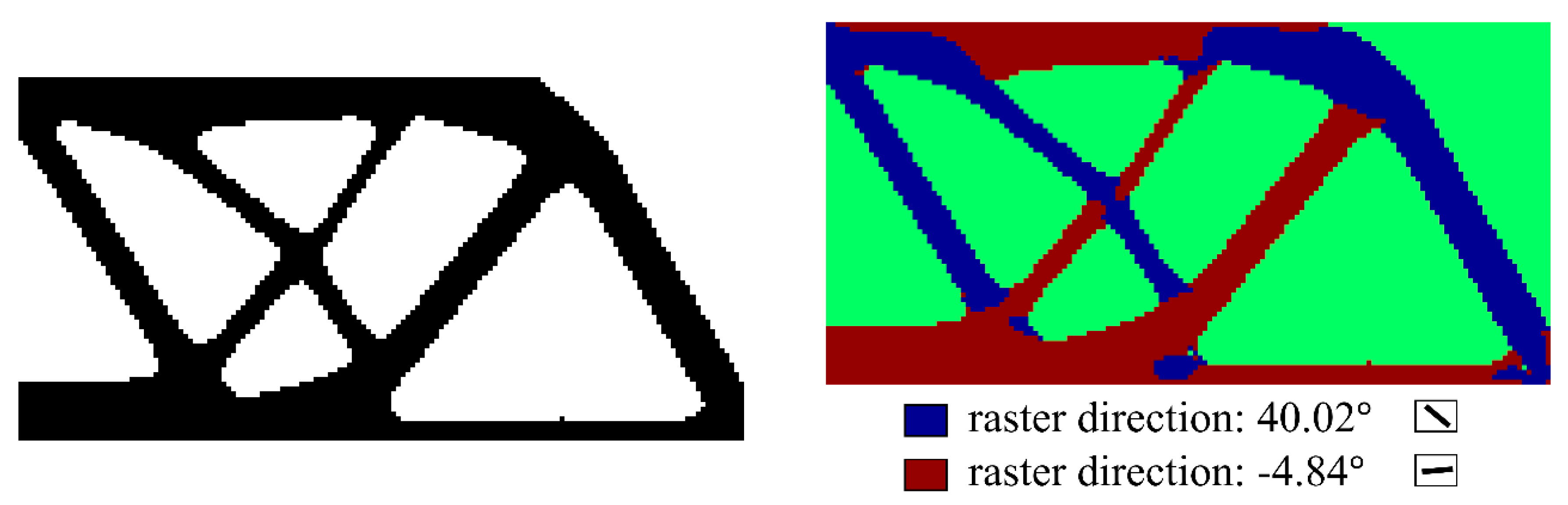
At the end, we would add a discussion about the initial-guess dependency issue. A finer mesh of 150 by 75 elements is used to perform the same topology optimization study with two designable raster directions. Initial setups of the level set function, density variables and raster directions all remain the same. Then, the optimization results are demonstrated in Figure 13. The optimized raster directions are 40.02° for the blue colored area and 4.84° for the red colored area. By comparing Figure 12a and Figure 13, we can see that both the structural geometry and the raster directions are very close. The reason is that, the same initial guess of hole distribution is adopted for the two optimization schemes, while for the level set method, the design result is more sensitive to the initial artificial hole distribution instead of the mesh scale. Even so, the optimization with a finer mesh takes 165 iterations to converge which consumes 10 more iterations than the case with a coarse mesh; and the structural compliance of the finer mesh optimization is 1.51% smaller. The computing time of the finer mesh optimization is 675s.
6. Conclusions
A hybrid topology optimization technique is presented in this paper in which the level set and DMO approaches are simultaneously applied to design and optimize the multipatch FDM parts. With the proposed technique, the concurrent material domain optimization, material domain decomposition with distinguished raster directions, and multiraster angle optimization have been realized. The effectiveness has been proven by a few case studies. In particular, aided by the proposed asynchronous starting strategy, the local misconvergence phenomenon of material domain decomposition has been successfully eliminated. It has also been observed that, the more patches simultaneously involved, the better the design performance will be.
In the future, the optimally designed parts are expected to be printed out so that their structural performance can be validated through experimental tests. In addition, the potential extension to multi-material, multipatch additive manufacturing will be explored. In the current study, a unidirectional zigzag deposition path is defined inside each patch for the sake of simplicity. In fact, the deposition path pattern of each patch can be extended to more complex patterns other than the zig-zag to achieve an even better design performance. Therefore, this aspect will be explored in our future work as well.
Author Contributions
Conceptualization, H.Y. and R.A.; methodology, H.Y. and H.H.; software, H.Y. and S.C.; validation, H.Y., H.H. and R.A.; formal analysis, H.Y.; investigation, H.Y.; resources, H.Y.; data curation, H.Y. and S.C.; writing—original draft preparation, H.Y. and H.H.; writing—review and editing, H.H. and R.A.; visualization, H.Y.; supervision, R.A.; project administration, H.Y.; funding acquisition, H.Y. All authors have read and agreed to the published version of the manuscript.
Funding
This work was supported by National Natural Science Foundation of China under Grant 51905537 and Hunan Provincial Natural Science Foundation of China under Grant 2019JJ50717.
Acknowledgments
The authors would like to thank the reviewers who take the time to review the paper and provide valuable inputs that enhance its quality.
Conflicts of Interest
The authors declare no conflict of interest.
References
- Gao, W.; Zhang, Y.; Ramanujan, D.; Ramani, K.; Chen, Y.; Williams, C.B.; Wang, C.C.L.; Shin, Y.C.; Zhang, S.; Zavattieri, P.D. The status, challenges, and future of additive manufacturing in engineering. Comput. Aided Des. 2015, 69, 65–89. [Google Scholar] [CrossRef]
- Liu, J.; Gaynor, A.T.; Chen, S.; Kang, Z.; Suresh, K.; Takezawa, A.; Li, L.; Kato, J.; Tang, J.; Wang, C.C.L.; et al. Current and future trends in topology optimization for additive manufacturing. Struct. Multidiscip. Optim. 2018, 57, 2457–2483. [Google Scholar] [CrossRef] [Green Version]
- Liu, J.; Ma, Y. A survey of manufacturing oriented topology optimization methods. Adv. Eng. Softw. 2016, 100, 161–175. [Google Scholar] [CrossRef]
- Leary, M.; Merli, L.; Torti, F.; Mazur, M.; Brandt, M. Optimal topology for additive manufacture: A method for enabling additive manufacture of support-free optimal structures. Mater. Des. 2014, 63, 678–690. [Google Scholar] [CrossRef]
- Mirzendehdel, A.M.; Suresh, K. Support structure constrained topology optimization for additive manufacturing. Comput. Aided Des. 2016, 81, 1–13. [Google Scholar] [CrossRef] [Green Version]
- Liu, J.; To, A.C. Deposition path planning-integrated structural topology optimization for 3D additive manufacturing subject to self-support constraint. Comput. Aided Des. 2017, 91, 27–45. [Google Scholar] [CrossRef]
- Gaynor, A.T.; Guest, J.K. Topology optimization considering overhang constraints: Eliminating sacrificial support material in additive manufacturing through design. Struct. Multidiscip. Optim. 2016, 54, 1157–1172. [Google Scholar] [CrossRef]
- Guo, X.; Zhou, J.; Zhang, W.; Du, Z.; Liu, C.; Liu, Y. Self-supporting structure design in additive manufacturing through explicit topology optimization. Comput. Methods Appl. Mech. Eng. 2017, 323, 27–63. [Google Scholar] [CrossRef] [Green Version]
- Wang, Y.; Gao, J.; Kang, Z. Level set-based topology optimization with overhang constraint: Towards support-free additive manufacturing. Comput. Methods Appl. Mech. Eng. 2018, 339, 591–614. [Google Scholar] [CrossRef]
- Zhang, W.; Zhou, L. Topology optimization of self-supporting structures with polygon features for additive manufacturing. Comput. Methods Appl. Mech. Eng. 2018, 334, 56–78. [Google Scholar] [CrossRef]
- Liu, J.; Ma, Y. A new multi-material level set topology optimization method with the length scale control capability. Comput. Methods Appl. Mech. Eng. 2018, 329, 444–463. [Google Scholar] [CrossRef]
- Liu, J. Piecewise length scale control for topology optimization with an irregular design domain. Comput. Methods Appl. Mech. Eng. 2019, 351, 744–765. [Google Scholar] [CrossRef]
- Mohan, S.R.; Simhambhatla, S. Adopting feature resolution and material distribution constraints into topology optimisation of additive manufacturing components. Virtual Phys. Prototyp. 2019, 14, 79–91. [Google Scholar] [CrossRef]
- Zhang, W.; Li, D.; Zhang, J.; Guo, X. Minimum length scale control in structural topology optimization based on the Moving Morphable Components (MMC) approach. Comput. Methods Appl. Mech. Eng. 2016, 311, 327–355. [Google Scholar] [CrossRef]
- Lazarov, B.S.; Wang, F.; Sigmund, O. Length scale and manufacturability in density-based topology optimization. Arch. Appl. Mech. 2016, 86, 189–218. [Google Scholar] [CrossRef] [Green Version]
- Liu, J.; Zheng, Y.; Ahmad, R.; Tang, J.; Ma, Y. Minimum length scale constraints in multi-scale topology optimisation for additive manufacturing. Virtual Phys. Prototyp. 2019, 14, 229–241. [Google Scholar] [CrossRef]
- Ulu, E.; Korkmaz, E.; Yay, K.; Ozdoganlar, O.B.; Kara, L.B. Enhancing the structural performance of additively manufactured objects through build orientation optimization. J. Mech. Des. 2015, 137, 111410. [Google Scholar] [CrossRef]
- Zhang, P.; Liu, J.; To, A.C. Role of anisotropic properties on topology optimization of additive manufactured load bearing structures. Scr. Mater. 2017, 135, 148–152. [Google Scholar] [CrossRef]
- Chiu, L.N.S.; Rolfe, B.; Wu, X.; Yan, W. Effect of stiffness anisotropy on topology optimisation of additively manufactured structures. Eng. Struct. 2018, 171, 842–848. [Google Scholar] [CrossRef]
- Vogiatzis, P.; Chen, S.; Zhou, C. An open source framework for integrated additive manufacturing and level-set based topology optimization. ASME J. Comput. Inf. Sci. Eng. 2017, 17, 041012. [Google Scholar] [CrossRef]
- Zegard, T.; Paulino, G.H. Bridging topology optimization and additive manufacturing. Struct. Multidiscip. Optim. 2015, 53, 175–192. [Google Scholar] [CrossRef]
- Wang, J.; Li, Y.; Hu, G.; Yang, M. Lightweight research in engineering: A review. Appl. Sci. 2019, 9, 5322. [Google Scholar] [CrossRef] [Green Version]
- Sleesongsom, S.; Bureerat, S. Topology optimisation using MPBILs and multi-grid ground element. Appl. Sci. 2018, 8, 271. [Google Scholar] [CrossRef] [Green Version]
- Zhang, P.; Toman, J.; Yu, Y.; Biyikli, E.; Kirca, M.; Chmielus, M.; To, A.C. Efficient design-optimization of variable-density hexagonal cellular structure by additive manufacturing: Theory and validation. J. Manuf. Sci. Eng. 2015, 137, 021004. [Google Scholar] [CrossRef]
- Wang, X.; Zhang, P.; Ludwick, S.; Belski, E.; To, A.C. Natural frequency optimization of 3D printed variable-density honeycomb structure via a homogenization-based approach. Addit. Manuf. 2017, 20, 189–198. [Google Scholar] [CrossRef]
- Yu, H.; Huang, J.; Zou, B.; Shao, W.; Liu, J. Stress-constrained shell-lattice infill structural optimization for additive manufacturing. Virtual Phys. Prototyp. 2020, 15, 35–48. [Google Scholar] [CrossRef]
- Panesar, A.; Abdi, M.; Hickman, D.; Ashcroft, I. Strategies for functionally graded lattice structures derived using topology optimisation for additive manufacturing. Addit. Manuf. 2018, 19, 81–94. [Google Scholar] [CrossRef]
- Hu, Z.; Gadipudi, V.K.; Salem, D.R. Topology optimization of lightweight lattice structural composites inspired by cuttlefish bone. Appl. Compos. Mater. 2019, 26, 15–27. [Google Scholar] [CrossRef]
- Liu, J.; Chen, Q.; Liang, X.; To, A.C. Manufacturing cost constrained topology optimization for additive manufacturing. Front. Mech. Eng. 2019, 14, 213–221. [Google Scholar] [CrossRef]
- Liu, J.; Zheng, Y.; Ma, Y.; Qureshi, A.; Ahmad, R. A topology optimization method for hybrid subtractive–additive remanufacturing. Int. J. Precis. Eng. Manuf. Green Technol. 2019, 1–15. [Google Scholar] [CrossRef]
- Brackett, D.; Ashcroft, I.; Hague, R. Topology optimization for additive manufacturing. In Proceedings of the 22nd Annual International Solid Freeform Fabrication Symposium, Austin, TX, USA, 8–10 August 2011. [Google Scholar]
- Ahn, S.H.; Montero, M.; Odell, D.; Roundy, S.; Wright, P.K. Anisotropic material properties of fused deposition modeling ABS. Rapid Prototyp. J. 2002, 8, 248–257. [Google Scholar] [CrossRef] [Green Version]
- Rezaie, R.; Badrossamay, M.; Ghaie, A.; Moosavi, H. Topology optimization for fused deposition modeling process. Proc. CIRP 2013, 6, 521–526. [Google Scholar] [CrossRef] [Green Version]
- Hoglund, R.; Smith, D.E. Non-isotropic material distribution topology optimization for fused deposition modeling products. In Proceedings of the 26th Annual International Solid Freeform Fabrication Symposium, Austin, TX, USA, 10–12 August 2015. [Google Scholar]
- Jiang, D.; Hoglund, R.; Smith, D.E. Continuous fiber angle topology optimization for polymer composite deposition additive manufacturing applications. Fibers 2019, 7, 14. [Google Scholar] [CrossRef] [Green Version]
- Yan, X.; Xu, Q.; Hua, H.; Huang, D.; Huang, X. Concurrent topology optimization of structures and orientation of anisotropic materials. Eng. Optim. 2019, 1–14. [Google Scholar] [CrossRef]
- Liu, J.; Yu, H. Concurrent deposition path planning and structural topology optimization for additive manufacturing. Rapid Prototyp. J. 2017, 23, 930–942. [Google Scholar] [CrossRef]
- Liu, J.; Ma, Y.; Qureshi, A.J.; Ahmad, R. Light-weight shape and topology optimization with hybrid deposition path planning for FDM parts. Int. J. Adv. Manuf. Technol. 2018, 97, 1123–1135. [Google Scholar] [CrossRef]
- Dapogny, C.; Estevez, R.; Faure, A.; Michailidis, G. Shape and topology optimization considering anisotropic features induced by additive manufacturing processes. Comput. Methods Appl. Mech. Eng. 2019, 344, 626–665. [Google Scholar] [CrossRef] [Green Version]
- Almeida, J.H.S.; Bittrich, L.; Nomura, T.; Spickenheuer, A. Cross-section optimization of topologically-optimized variable-axial anisotropic composite structures. Compos. Struct. 2019, 225, 111150. [Google Scholar] [CrossRef]
- Zhou, X.; Hsieh, S.-J.; Ting, C.-C. Modelling and estimation of tensile behaviour of polylactic acid parts manufactured by fused deposition modelling using finite element analysis and knowledge-based library. Virtual Phys. Prototyp. 2018, 13, 177–190. [Google Scholar] [CrossRef]
- Srivastava, M.; Rathee, S. Optimisation of FDM process parameters by Taguchi method for imparting customised properties to components. Virtual Phys. Prototyp. 2018, 13, 203–210. [Google Scholar] [CrossRef]
- Huang, J.; Chen, Q.; Jiang, H.; Zou, B.; Li, L.; Liu, J.; Yu, H. A survey of design methods for material extrusion polymer 3D printing. Virtual Phys. Prototyp. 2020, 1–15. [Google Scholar] [CrossRef]
- Ahn, S.H.; Baek, C.; Lee, S.; Ahn, I.S. Anisotropic tensile failure model of rapid prototyping parts—Fused deposition modeling (FDM). Int. J. Mod. Phys. B 2003, 17, 1510–1516. [Google Scholar] [CrossRef]
- Lee, C.S.; Kim, S.G.; Kim, H.J.; Ahn, S.H. Measurement of anisotropic compressive strength of rapid prototyping parts. J. Mater. Process. Technol. 2007, 187–188, 627–630. [Google Scholar] [CrossRef]
- Hill, N.; Haghi, M. Deposition direction-dependent failure criteria for fused deposition modeling polycarbonate. Rapid Prototyp. J. 2014, 20, 221–227. [Google Scholar] [CrossRef]
- Umetani, N.; Schmidt, R. Cross-sectional structural analysis for 3D printing optimization. SIGGRAPH Asia Tech. Briefs 2013, 5. [Google Scholar] [CrossRef] [Green Version]
- Mirzendehdel, A.M.; Rankouhi, B.; Suresh, K. Strength-based topology optimization for anisotropic parts. Addit. Manuf. 2018, 19, 104–113. [Google Scholar] [CrossRef]
- Osher, S.; Fedkiw, R. Level Set Methods and Dynamic Implicit Surfaces; Applied Mathematical Sciences Book Series; Springer: New York, NY, USA, 2003; Volume 153. [Google Scholar]
- Osher, S.; Sethian, J.A. Fronts propagating with curvature-dependent speed: Algorithms based on Hamilton-Jacobi formulations. J. Comput. Phys. 1988, 79, 12–49. [Google Scholar] [CrossRef] [Green Version]
- Wang, M.Y.; Wang, X.; Guo, D. A level set method for structural topology optimization. Comput. Methods Appl. Mech. Eng. 2003, 192, 227–246. [Google Scholar] [CrossRef]
- Allaire, G.; Jouve, F.; Toader, A.-M. Structural optimization using sensitivity analysis and a level-set method. J. Comput. Phys. 2004, 194, 363–393. [Google Scholar] [CrossRef] [Green Version]
- Wang, M.Y.; Wang, X. ’Color’ level sets: A multi-phase method for structural topology optimization with multiple materials. Comput. Methods Appl. Mech. Eng. 2004, 193, 469–496. [Google Scholar] [CrossRef]
- Wang, M.Y.; Wang, X. A level-set based variational method for design and optimization of heterogeneous objects. Comput. Aided Des. 2005, 37, 321–337. [Google Scholar] [CrossRef]
- Wang, Y.; Luo, Z.; Kang, Z.; Zhang, N. A multi-material level set-based topology and shape optimization method. Comput. Methods Appl. Mech. Eng. 2015, 283, 1570–1586. [Google Scholar] [CrossRef]
- Cui, M.; Chen, H.; Zhou, J. A level-set based multi-material topology optimization method using a reaction diffusion equation. Comput. Aided Des. 2016, 73, 41–52. [Google Scholar] [CrossRef]
- Stegmann, J.; Lund, E. Discrete material optimization of general composite shell structures. Int. J. Numer. Methods Eng. 2005, 62, 2009–2027. [Google Scholar] [CrossRef]
- Lund, E.; Stegmann, J. On structural optimization of composite shell structures using a discrete constitutive parametrization. Wind Energy 2005, 8, 109–124. [Google Scholar] [CrossRef]
- Ferreira, R.T.L.; Rodrigues, H.C.; Guedes, J.M.; Hernandes, J.A. Hierarchical optimization of laminated fiber reinforced composites. Compos. Struct. 2014, 107, 246–259. [Google Scholar] [CrossRef]
- Garland, A.; Fadel, G. Optimizing topology and gradient orthotropic material properties under multiple loads. J. Comput. Inf. Sci. Eng. 2019, 19, 021007. [Google Scholar] [CrossRef]
Figure 1.
Single printing layer with multiple raster directions represented by the yellow arrows.
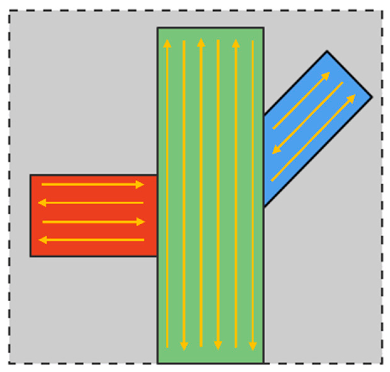
Figure 2.
Levels of the design freedom.
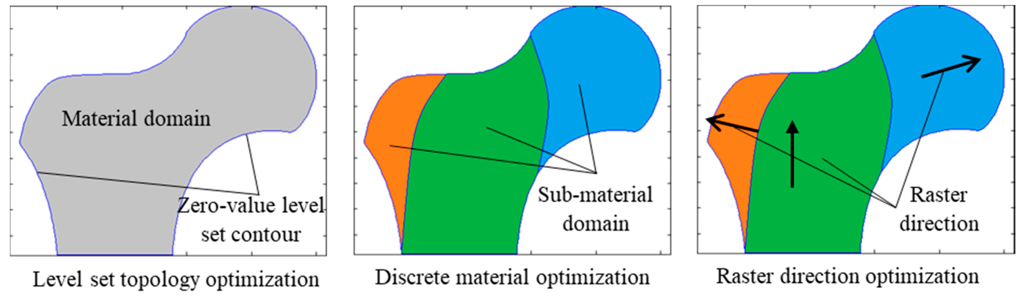
Figure 3.
Flow chart of the solution process.
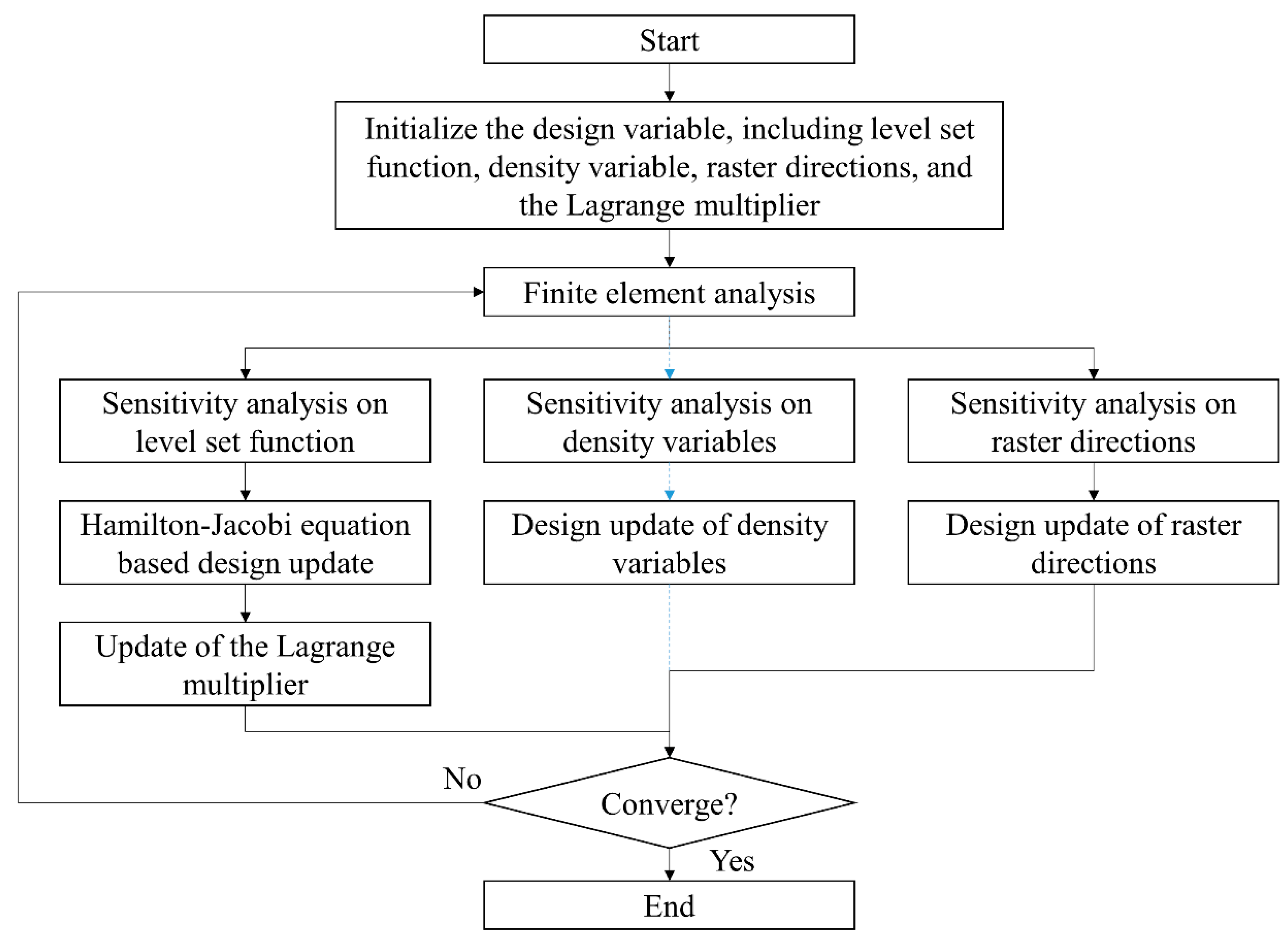
Figure 4.
Misconverged local areas. (a) Cantilever problem; (b) short cantilever problem.
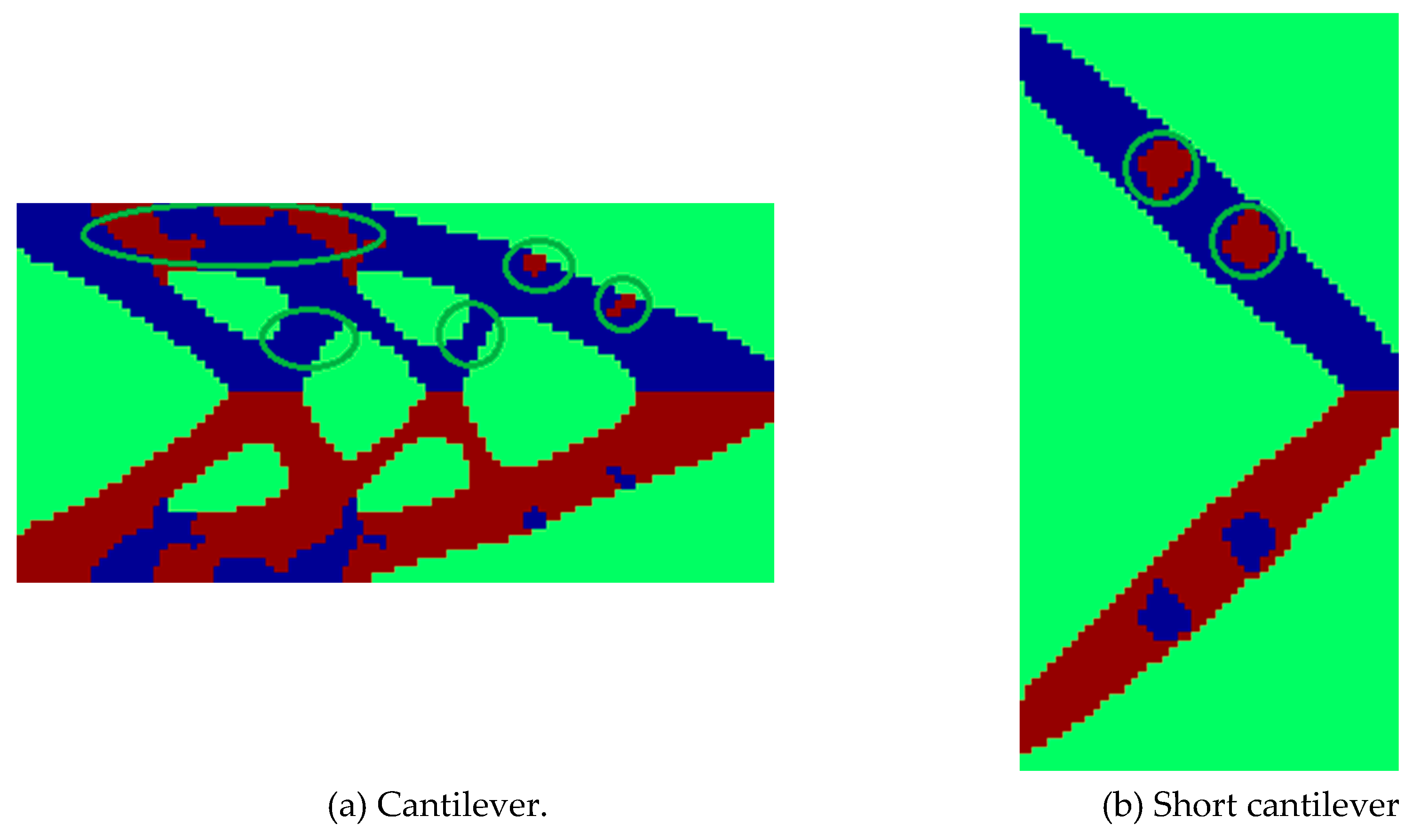
Figure 5.
Schematic of the cantilever problem definition.
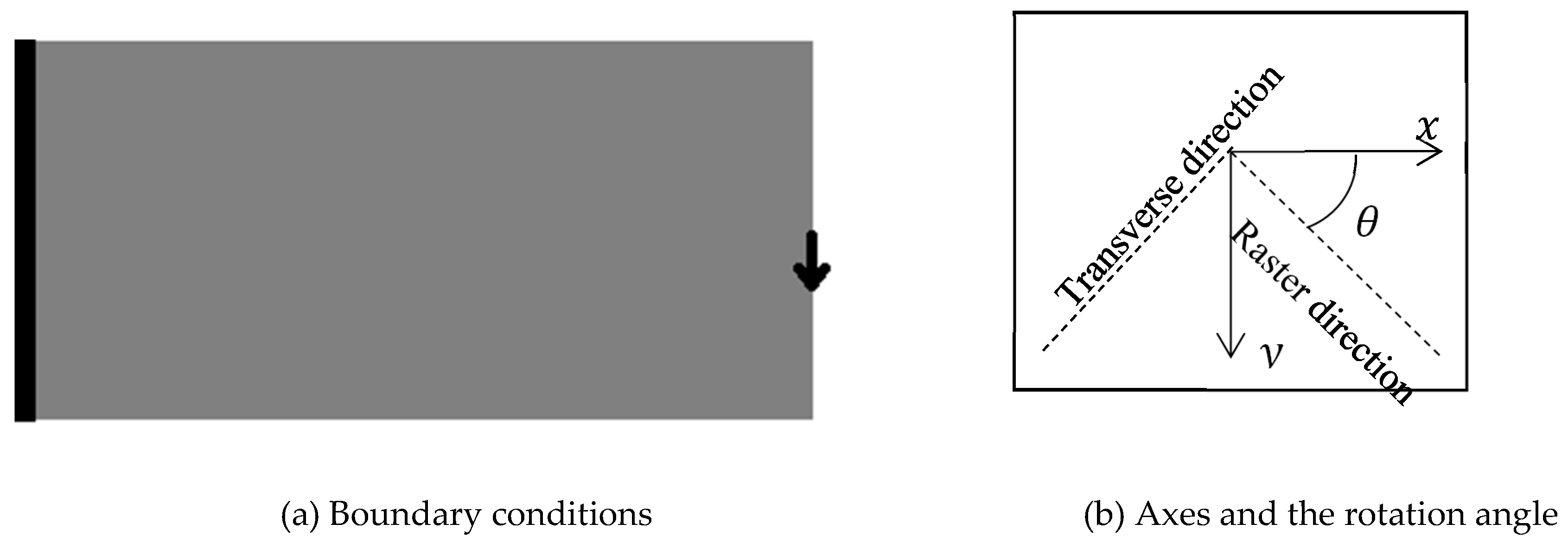
Figure 6.
Cantilever optimization results (the blue color shows the converged , the red color shows the converged , and the green color shows the misconverged or void areas).
Figure 6.
Cantilever optimization results (the blue color shows the converged , the red color shows the converged , and the green color shows the misconverged or void areas).
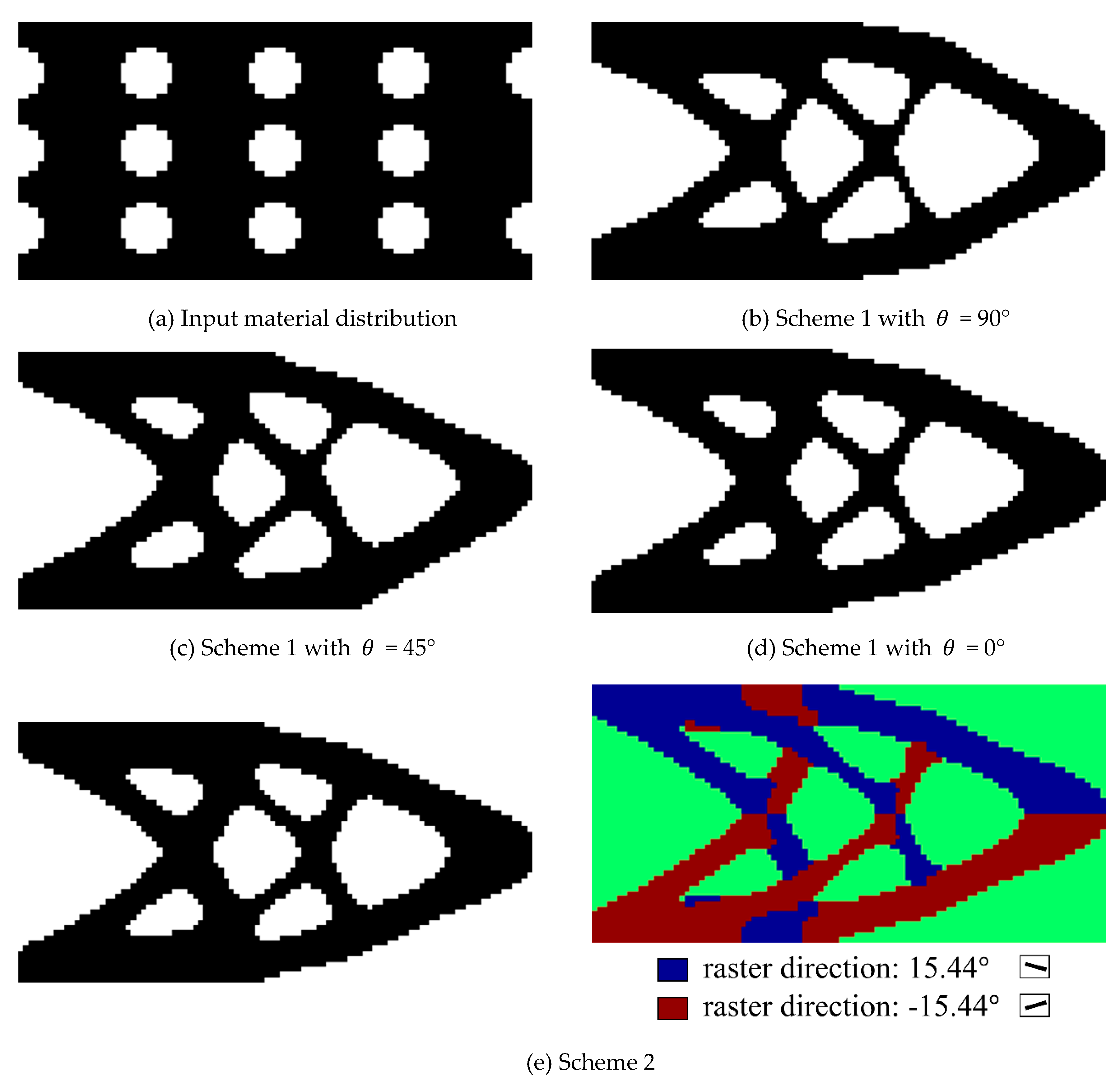
Figure 7.
Schematic of the short cantilever problem definition.
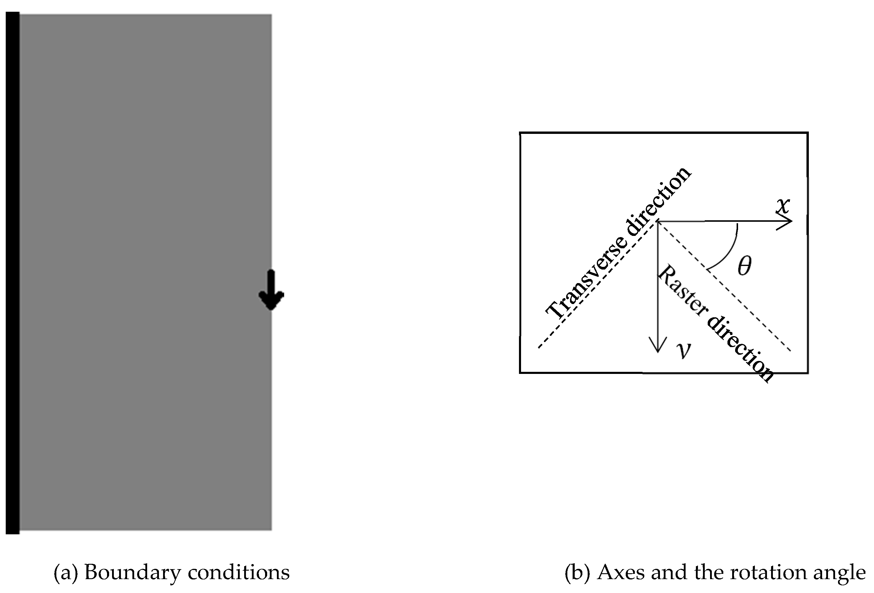
Figure 8.
Short cantilever optimization results (the blue color shows the converged , the red color shows the converged , and the green color shows the misconverged or void areas).
Figure 8.
Short cantilever optimization results (the blue color shows the converged , the red color shows the converged , and the green color shows the misconverged or void areas).

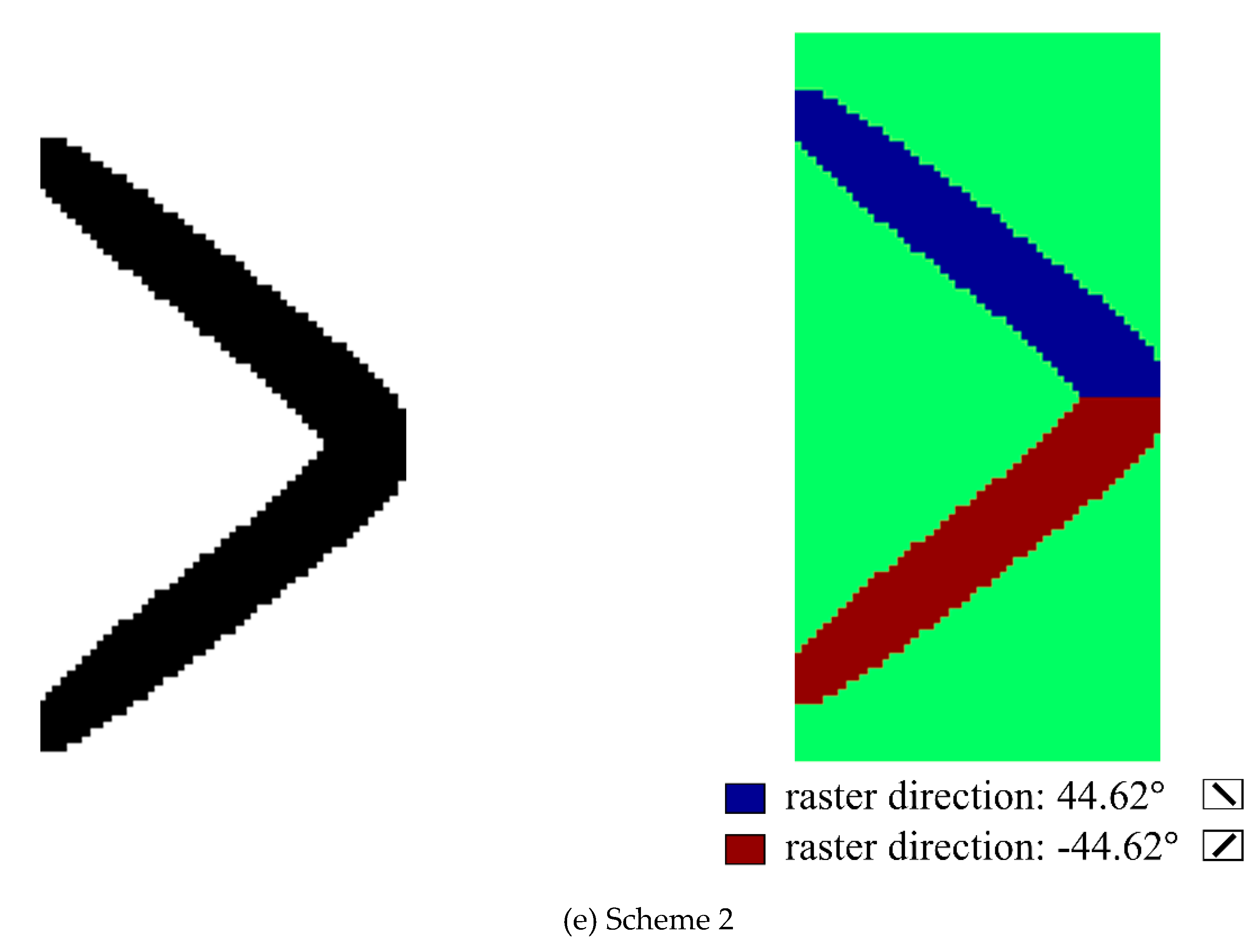
Figure 9.
Schematic of the Michell structure problem definition.
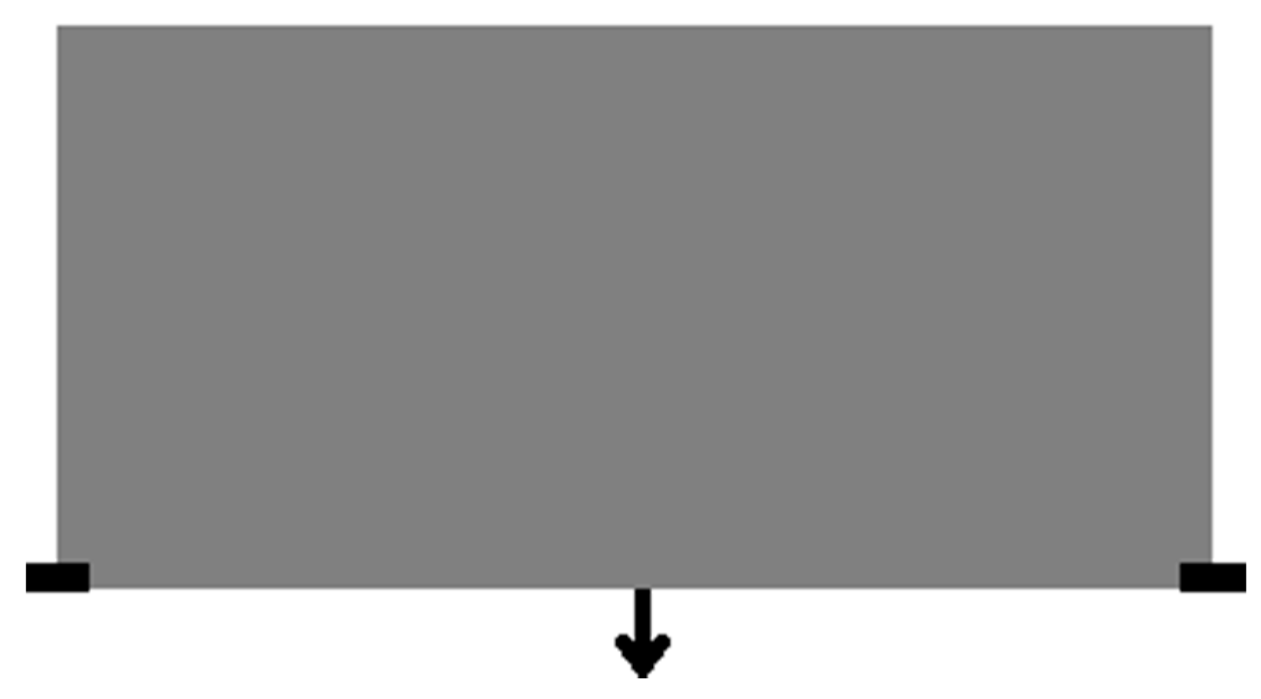
Figure 10.
Structure optimization results (the blue color shows the converged , the red color shows the converged , the yellow color shows the converged , and the green color shows the misconverged or void areas).
Figure 10.
Structure optimization results (the blue color shows the converged , the red color shows the converged , the yellow color shows the converged , and the green color shows the misconverged or void areas).
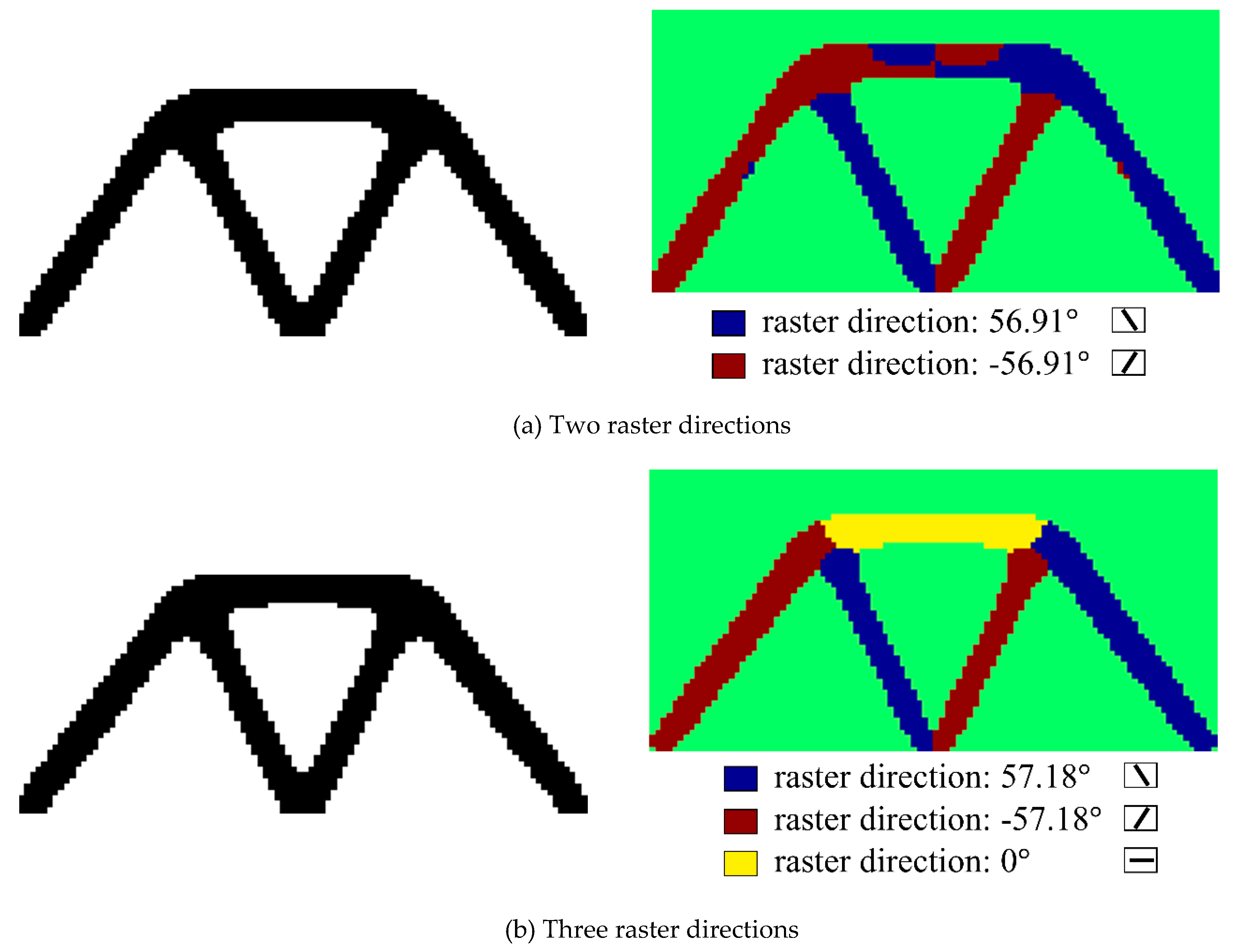
Figure 11.
Schematic of the MBB structure problem definition.
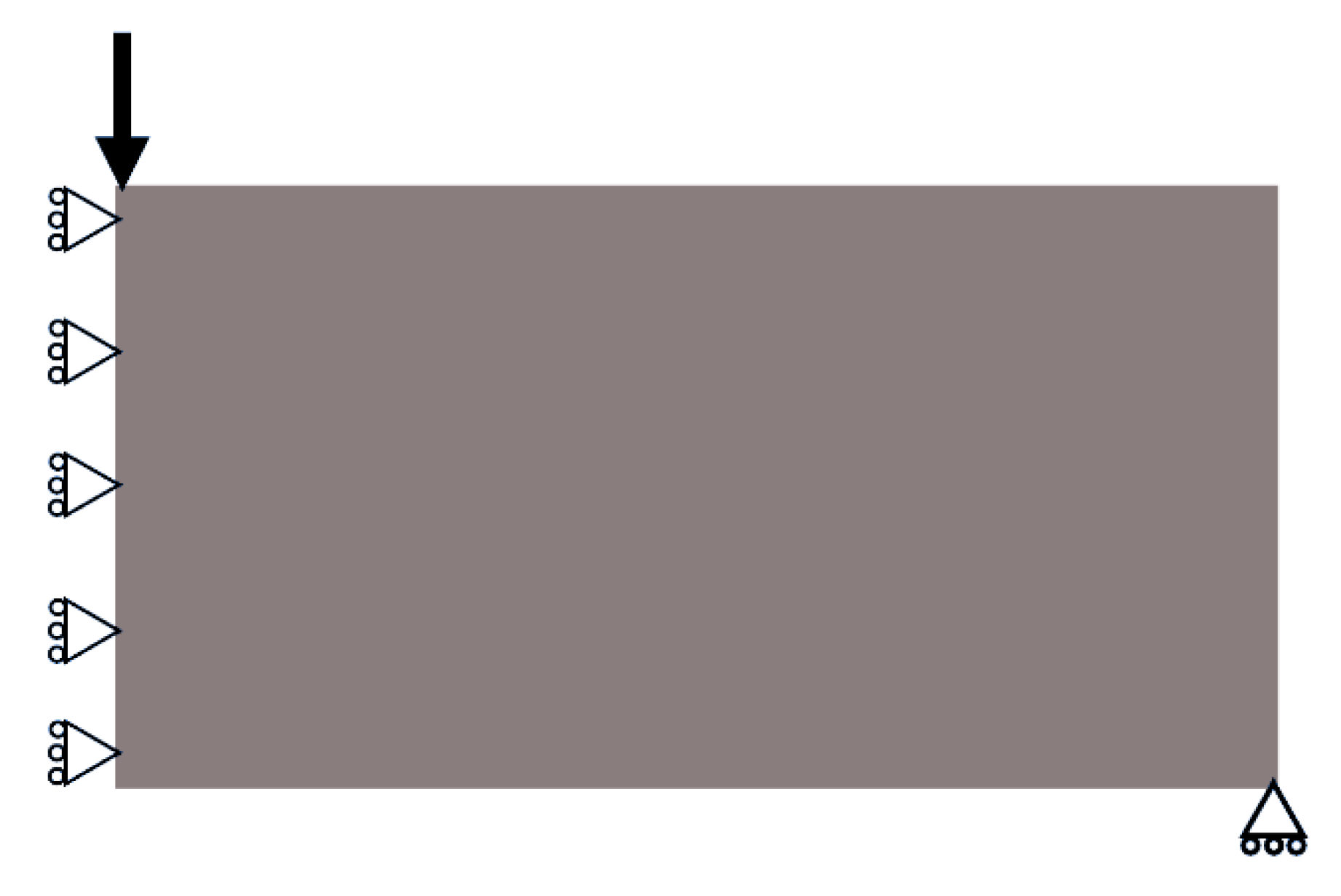
Figure 12.
MBB structure optimization results (the blue color shows the converged , the red color shows the converged , the yellow color shows the converged , and the green color shows the misconverged or void areas).
Figure 12.
MBB structure optimization results (the blue color shows the converged , the red color shows the converged , the yellow color shows the converged , and the green color shows the misconverged or void areas).
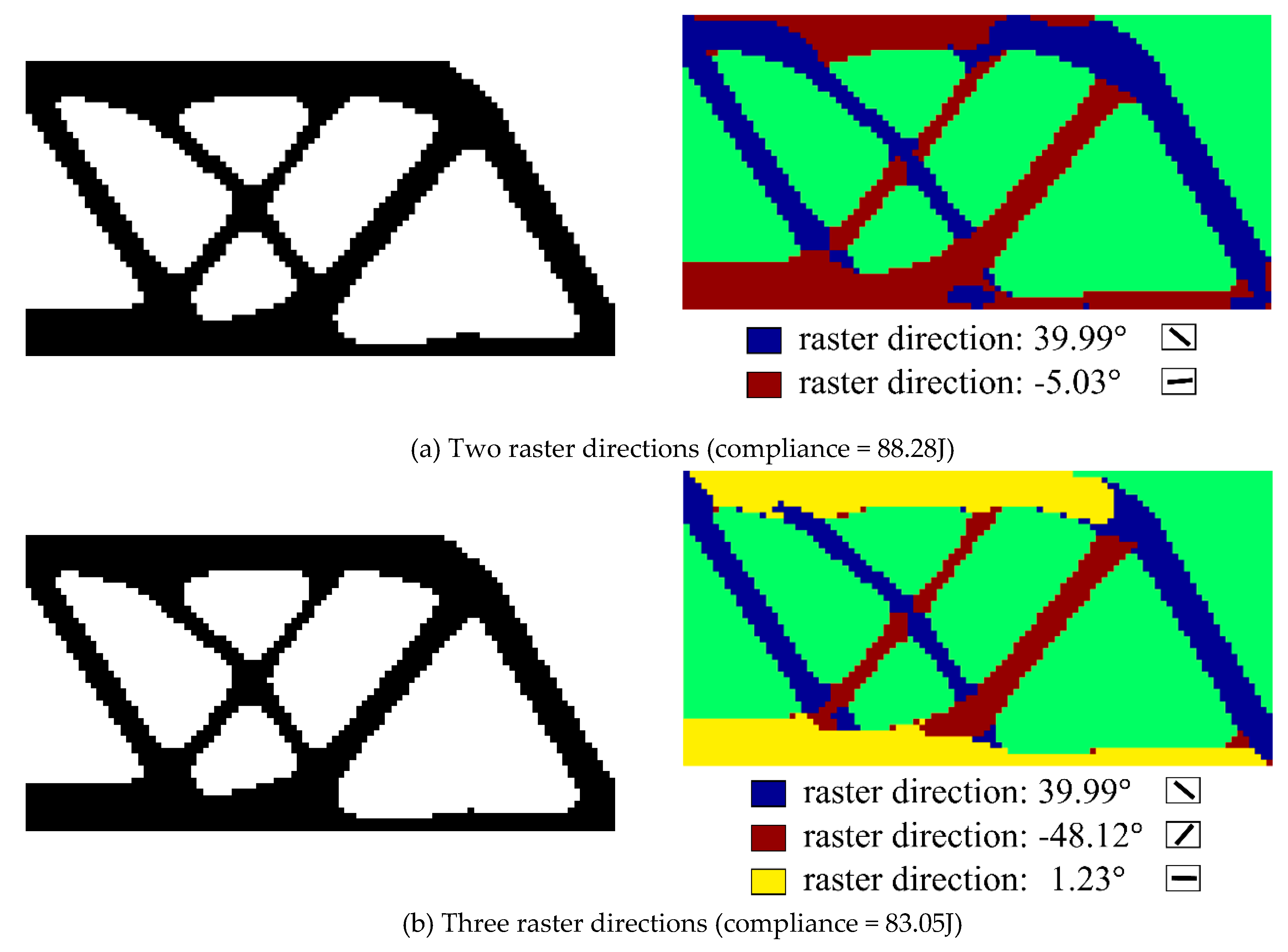
Figure 13.
MBB structure optimization result with a finer mesh (compliance = 86.95J). (The blue color shows the converged , the red color shows the converged , and the green color shows the misconverged or void areas).
Figure 13.
MBB structure optimization result with a finer mesh (compliance = 86.95J). (The blue color shows the converged , the red color shows the converged , and the green color shows the misconverged or void areas).

Table 1.
Data of The Cantilever Optimization Results.
| = 90° | = 45° | = 0° | Scheme 2 | |
|---|---|---|---|---|
| Structural compliance (J) | 76.67 | 69.91 | 57.94 | 55.47 |
| Compliance reduction compared to the worst case | 0% | 8.82% | 24.43% | 27.65% |
| Optimal raster directions | 90° | 45° | 0° | ±15.44° |
Table 2.
Data of The Cantilever Optimization Results.
| = 90° | = 45 | = 0° | Scheme 2 | |
|---|---|---|---|---|
| Structural compliance (J) | 11.31 | 12.02 | 11.48 | 8.12 |
| Compliance reduction compared to the worst case | 5.91% | 0% | 4.49% | 32.44% |
| Optimal raster directions | 90° | 45° | 0° | ±44.62° |
© 2020 by the authors. Licensee MDPI, Basel, Switzerland. This article is an open access article distributed under the terms and conditions of the Creative Commons Attribution (CC BY) license (http://creativecommons.org/licenses/by/4.0/).
Share and Cite
MDPI and ACS Style
Yu, H.; Hong, H.; Cao, S.; Ahmad, R. Topology Optimization for Multipatch Fused Deposition Modeling 3D Printing. Appl. Sci. 2020, 10, 943. https://doi.org/10.3390/app10030943
AMA Style
Yu H, Hong H, Cao S, Ahmad R. Topology Optimization for Multipatch Fused Deposition Modeling 3D Printing. Applied Sciences. 2020; 10(3):943. https://doi.org/10.3390/app10030943
Chicago/Turabian StyleYu, Huangchao, Huajie Hong, Su Cao, and Rafiq Ahmad. 2020. "Topology Optimization for Multipatch Fused Deposition Modeling 3D Printing" Applied Sciences 10, no. 3: 943. https://doi.org/10.3390/app10030943
Note that from the first issue of 2016, this journal uses article numbers instead of page numbers. See further details here.