A Probabilistic Capacity Model and Seismic Vulnerability Analysis of Wall Pier Bridges

Abstract

This study aims to establish a probabilistic capacity model of a wall pier under various damage states, and the seismic vulnerability of a typical wall pier bridge is studied. The finite element analysis of the wall pier is carried out by using the layered shell element, and its accuracy is verified through the comparison with the experimental results. A series of wall pier samples are generated based on the survey data, and the corresponding finite element models are established. The hysteresis analysis is implemented to obtain the displacement drift ratio of each seismic performance point. A candidate capacity model with various factors is proposed, and the unknown parameters are estimated and filtered by the Bayesian method. One hundred and twenty bridge samples of a benchmark bridge are generated by considering the uncertainty of parameters, and the finite element models are established. The bridge samples and ground motions were matched by one-to-one correspondence for the nonlinear time history analysis, and seismic vulnerability models of bridge components and system are obtained. The results showed that the in-plane capacity of wall piers is mainly affected by axial compression ratio, shear span ratio, and vertical reinforcement ratio. The wall pier shows excellent behavior in the earthquakes. The capacity models of wall piers can be used for evaluating the damage states of wall piers, and obtaining the seismic vulnerability model of wall piers bridges to be used for future seismic risk assessment and retrofit prioritization.

1. Introduction

Seismic damage of bridge structures will cause not only serious economic losses but also significant difficulties in disaster relief and post-disaster reconstruction. The bridge vulnerability model can evaluate the damage probabilities of bridge structures during an earthquake, which can be used not only for the seismic risk assessment, but also for the sorting of the bridge structure reinforcements. The wall pier girder bridge is a universal bridge type of municipal bridges in China. So far, few studies about wall pier bridges have been published [1,2]. There are some gaps to be filled: (1) Formerly used finite elements such as fiber-based beam-column element are not quite suitable for the simulation of wall piers, and some newly-developed finite elements have not been applied to this field; (2) The seismic capacity models of common pier columns developed in previous studies cannot be applied to the wall pier, a parameter-dependent capacity model is worth further developing. In this study, these problems are analyzed and discussed, and a seismic vulnerability model of the wall pier girder bridge is proposed.

There are significant differences between the wall piers and common column piers in seismic behavior and failure mode due to their distinguishing geometric details. Haroun [3] and Aboutaha [4] conducted experimental studies on wall piers in 1993 and 1999, respectively. Haroun studied the wall pier bridges built before 1971 in California, then established experimental components of wall piers and found out that in-plane shear failure and out-of-plane flexural failure occurred in the wall piers under cyclic load. Aboshadi investigated the wall pier girder bridges in the United States and established seven wall pier experimental components that were subjected to out-of-plane cyclic loading, with the result that flexural failure occurred in all experimental components. The results reported here reflect that different failure modes may appear in both the in-plane and out-of-plane of the wall piers under the action of loads. In view of this mechanical property of the wall pier, finite element models of the wall piers are established by the layered shell element in this study, and their accuracy is verified. Since few studies were focused on wall piers, this study refers to several experimental studies of shear walls considering the similarity between the structures of the wall pier and the shear wall. Greifenhagen [5] conducted an experimental study on four shear walls with insufficient vertical reinforcement. None of these components suffered a complete brittle failure, and the strength of these components was controlled by bending strength. The axial compression ratio had a significant influence on the displacement capacity of the components. Hidalgo et al. [6] studied the seismic performance of the low-rise shear wall and conducted hysteresis analysis on the components with different shear span ratios, reinforcement ratios and compressive strengths of concrete, then found that all the structural parameters had a significant influence on displacement drift ratios of the components under various damage states.

Based on the studies above, this article proposes an in-plane probabilistic capability model of wall piers with structural parameters and other information. Utilizing the sample points obtained by numerical simulation, estimate and filter the unknown parameters of the capability model by Bayesian parameter estimation method. For a wall pier girder bridge as a reference bridge, 120 wall pier girder bridge samples were obtained by Latin hypercube sampling by considering the uncertainty of the chosen parameters. One hundred and twenty finite element models of these samples are subjected to one earthquake event, respectively, by means of time-history analysis. On this basis, the seismic demand of each vulnerable component is obtained. The in-plane capacity models of the wall piers are used to determine its damage state. The out-of-plane damage states of the wall piers and the damage states of other vulnerable components are determined by referring to previous studies. The seismic vulnerabilities of the components are obtained by using maximum likelihood estimation method. [7] It is based on the damage samples which generated from abovementioned demand samples and capacity samples, and the corresponding IM values The bridge system is regarded as a series system to calculate its seismic vulnerability.

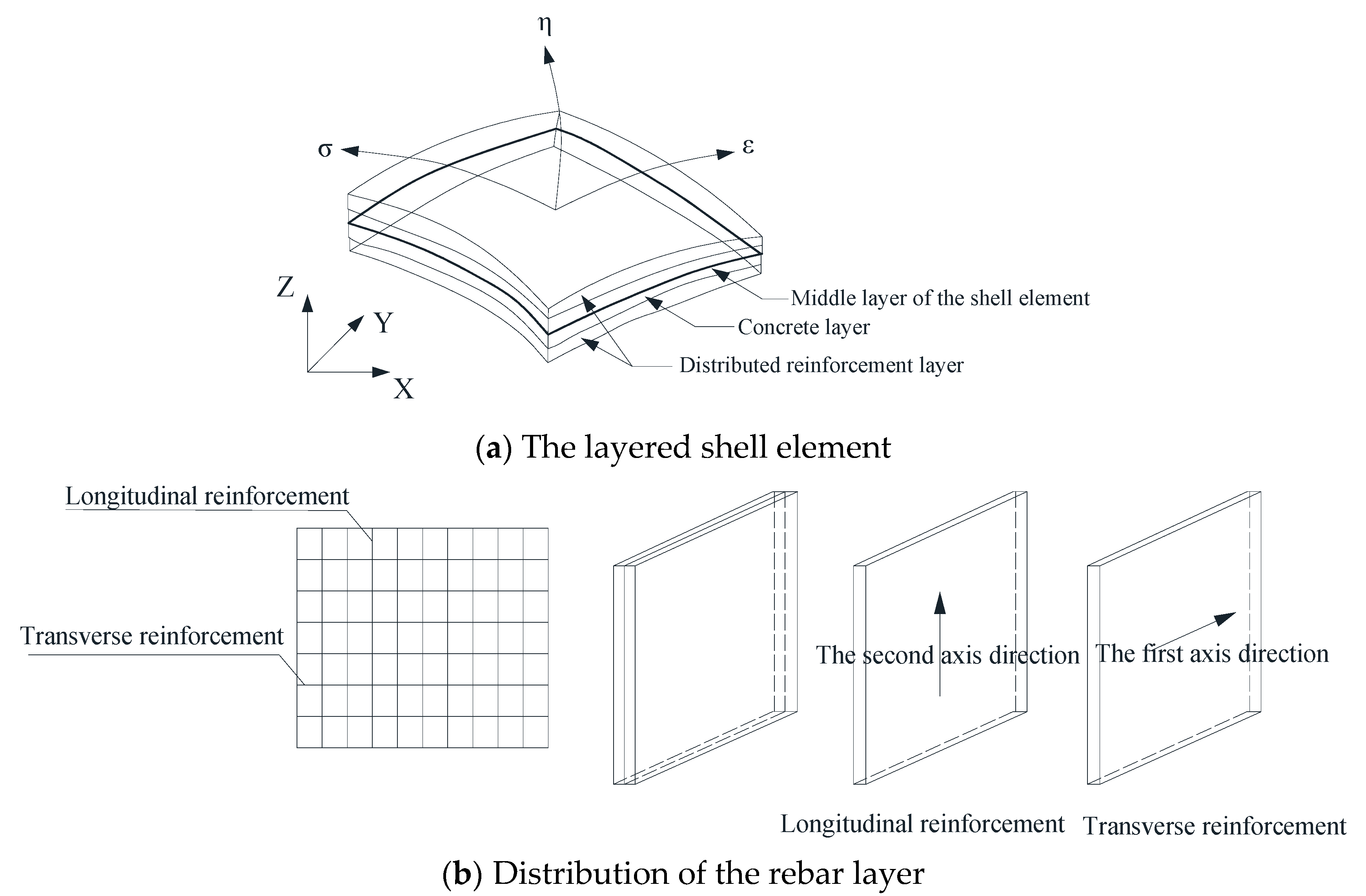
2. Finite Element Model of Wall Pier

Referring to previous studies on pier columns and shear wall components, we explore more accurate simulation methods in this study. For common pier columns, the series models [8,9] are often used to simulate the bending-shear effects of pier columns. Fiber beam-column elements are used to simulate the bending effects of piers, while zero-length spring elements are used to simulate shear effects and connect them in series to simulate the bending-shear effects. Bending-shear coupling is the key to this model [10]. In previous studies, the relationship between shear deformation and bending deformation of piers at failure was obtained mainly through statistically analyzing the experimental results, and this relationship was taken as the basis of bending-shear coupling. Considering the lack of experimental data of wall piers, the series models are not supposed to simulate wall piers appropriately. Multi-vertical-line elements and layered shell elements are mostly used to model shear walls [11,12]. While in multi-vertical-line element models, multiple vertical bars are used to simulate the bending, tensile and compressive effects of the shear wall structures, and horizontal springs are used to simulate the shear effects [13]. However, this model cannot simulate the out-of-plane mechanical properties of the structures.

With reference to mechanics of composite materials, layered shell models [14] are divided into several layers in the direction of thickness according to actual structure, and the corresponding material properties are assigned to each layer, as shown in Figure 1. Through the definition of strain and curvature of the central layer, the internal force of the layered shell element is obtained by numerical integration according to the plane hypothesis and material constitutive relation. The coupling between in-plane bending, in-plane shearing and out-of-plane bending can be considered in the layered shell model. In conclusion, the layered shell element model is selected to analyze the wall pier in this study, and its accuracy is verified by previous test results.

Based on OpenSees platform, Lu et al. [14] developed a new layered shell section, which was assigned to element ShellMITC4, to build a layered shell element. Due to the lack of experimental wall pier data, this study selected experimental components similar to wall piers from previous studies on shear walls [15] and from studies on pier columns in the PEER database [16]. The experimental results and the numerical simulation results are then compared to verify the accuracy of this simulation. The parameters of these selected components are shown in

Table 1. Parameters of shear wall components.

Component Name	Section Size (cm) (Height × Width × Thickness)	Concrete Strength	Embedded Column Width (cm)	Axial Compression Ratio	Dark Column Reinforcement Ratio		Structural Reinforcement		Destruction Form
					Vertical	Lateral	Vertical	Lateral
SW1-1	200 × 100 × 12.5	C30	20	0.1	1.84%	0.57%	0.38%	0.36%	Bending
SW2-1	100 × 100 × 12.5	C40	20	0.3	1.84%	0.57%	0.38%	0.36%	Shearing

and

Table 2. Parameters of column components.

Component Name	Section Size (cm) (Height × Width × Thick)	Concrete Strength (MPa)	Axial Compression Ratio	Reinforcement Ratio	Destruction Form
Park and Paulay	178 × 60 × 40	26.9	0.1	Vertical 1.88% Transverse 2.2%	bending damage
Wehbe	234 × 61 × 38	27.2	0.098	Vertical 2.22% Transverse 0.4%	bending damage
Wight03	88 × 31 × 15	26.1	0.147	Vertical 2.45% Transverse 0.5%	bending and shearing
Wight04	88 × 31 × 15	26.1	0.147	Vertical 2.45% Transverse 0.5%	bending and shearing

respectively:

The finite element model is divided into elements with an aspect ratio of approximately 1.0, and the steel bars disposed in the test pieces are simulated by the dispersed steel layer. The nodes at the bottom of the component are fixed, and vertical and horizontal loads are applied at the top, where the horizontal loads are loaded by displacement control. A comparison between simulation and experimental results is shown in Figure 2. From (a) and (b) in Figure 2, it can be seen that the yield and plastic development of the structure, as well as the peak and decline stages of the bearing capacity, can be well simulated by this numerical model. The hysteretic curves of numerical simulations compare well with that of experiments. Observing the experimental results of (c)~(f) in Figure 2, it can be inferred that the four components show good ductility mainly due to the relatively large shear span ratio. By comparing the experimental and calculated values in the four figures, conclusion that the numerical simulation can well reflect the development of structural strength and the peak of bearing capacity is inferred. However, in plastic development stage, there is a steep descending segment in the capacity curves from the numerical simulation results (Figure 2b), which is not consistent with the experimental results. By recording the concrete strain of the shell element on the outer surface at the pier bottom, it is found that the concrete strain reaches its limit threshold, that is, concrete crushed too early. The possible influencing factors behind this may be attributed to the aspect ratio of the cross-section and the discretizing number of reinforcing bars. There are certain errors in some special cases by using the layered shell element, but in general, the layered shell element can well simulate different failure modes of the wall-shaped components.

3. Probabilistic Capability Model of Wall Piers

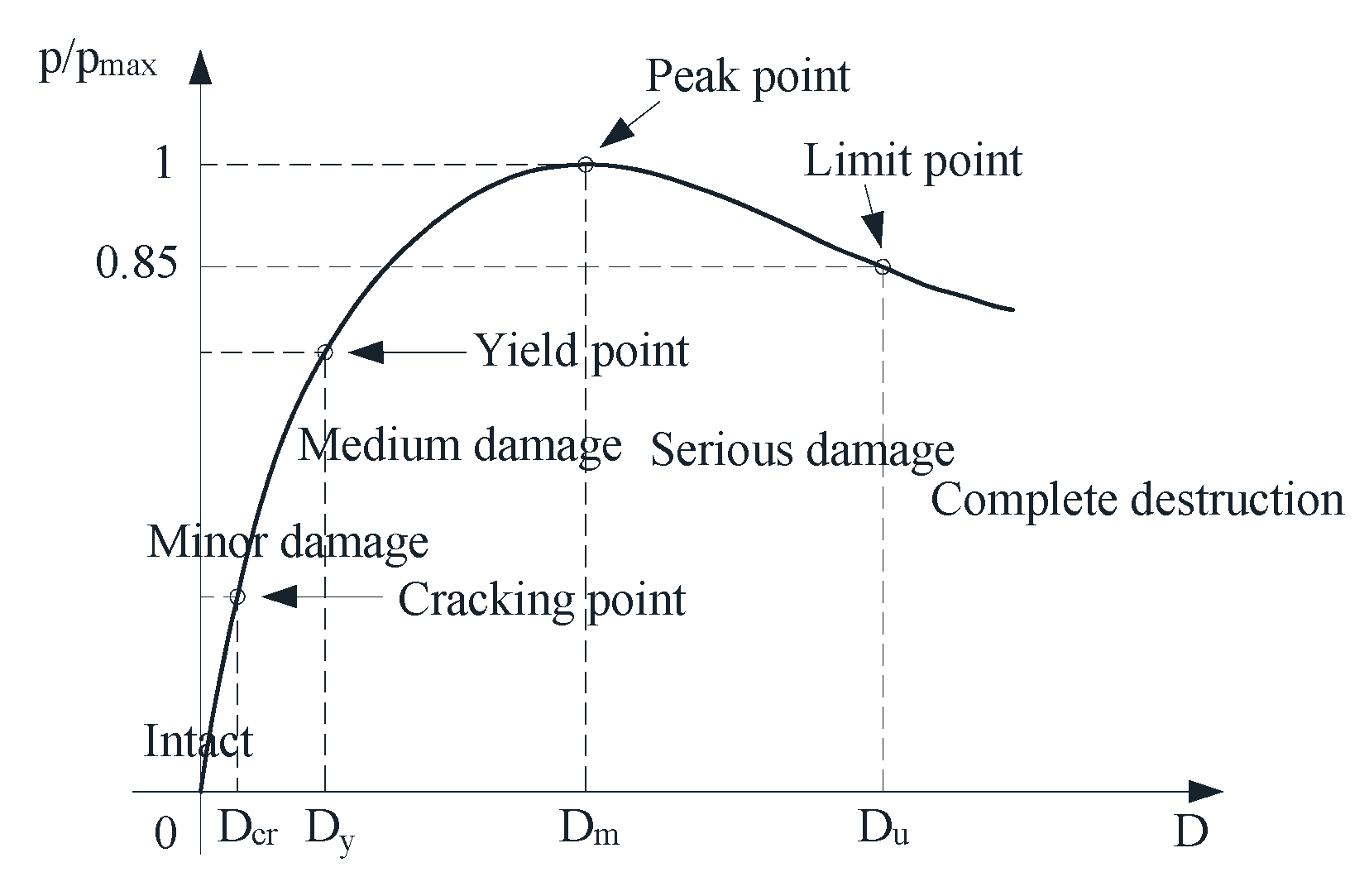
3.1. Wall Pier Damage Indexes

As a part of the performance-based structural seismic design, performance level definition also plays an important role in seismic vulnerability analysis. A structural performance level can be defined as the maximum degree of expected structure damage for a given earthquake intensity. According to previous studies [17], a five-performance-level classification is adopted for the wall pier girder bridges in this study. That is intact, minor damage, medium damage, severe damage, and complete destruction. The depiction of the pier damage states is shown as Figure 3, plotted by displacements on the horizontal and normalized lateral load on the vertical.

Commonly used damage indices for pier components include material strain, ductility coefficient, two-parameter damage model, displacement drift ratio, etc. The displacement drift ratio is selected as the damage index of wall piers in this study considering the peculiarity of wall piers and the simplicity of the analysis. The displacement drift ratios when the components are cracked, yielded, and the structural bearing capacity reaches the peak and limit states are taken as the boundary point of each damage state.

The out-of-plane performances of the wall piers are similar to that of the common pier columns. Therefore, the limit values of each out-of-plane damage state directly refer to previous research results [18] of the common pier columns, as shown in

Table 3. Division of each damage state to the wall pier in out of plane.

Performance Level	Degree of Damage	Seismic Performance Index
level 1	Intact	MDR ≤ 0.11%
level 2	Minor damage	0.11% < MDR ≤ 0.38%
level 3	Medium damage	0.38% < MDR ≤ 0.84%
level 4	Serious damage	0.84% < MDR ≤ 2.23%
level 5	Complete destruction	MDR > 2.23%

, where MDR denotes the displacement drift ratio, which is defined as follows:

$$MDR=D/H$$

(1)

where D is the displacement at the top of the pier and H is the net height of the pier. Considering that the in-plane performance of wall piers is quite different to that of common pier columns, numerical simulation is used to obtain the values of each in-plane performance point. By adopting the Bayesian stepwise regression method, the formulas of different performance points are obtained considering the impact of some factors.

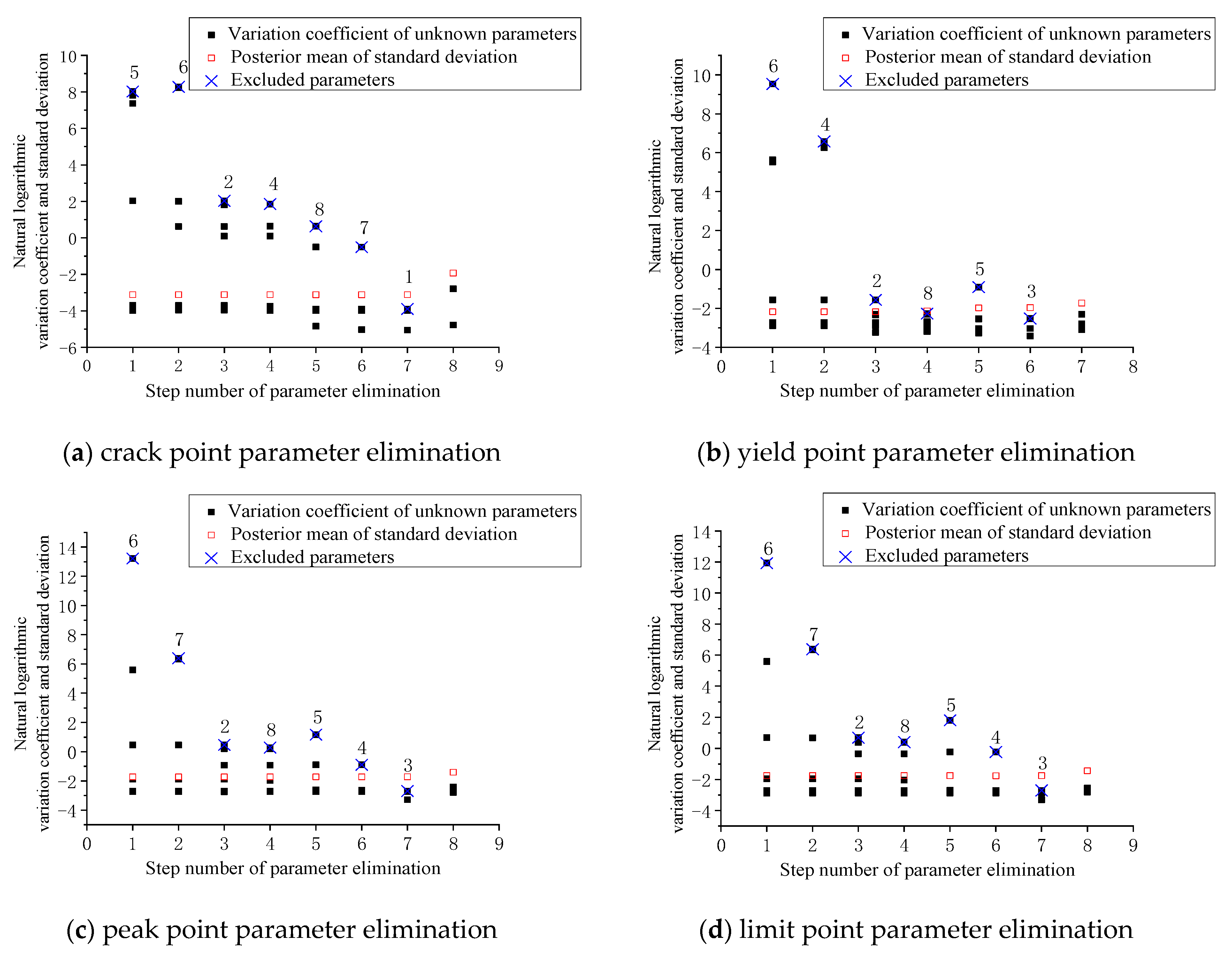
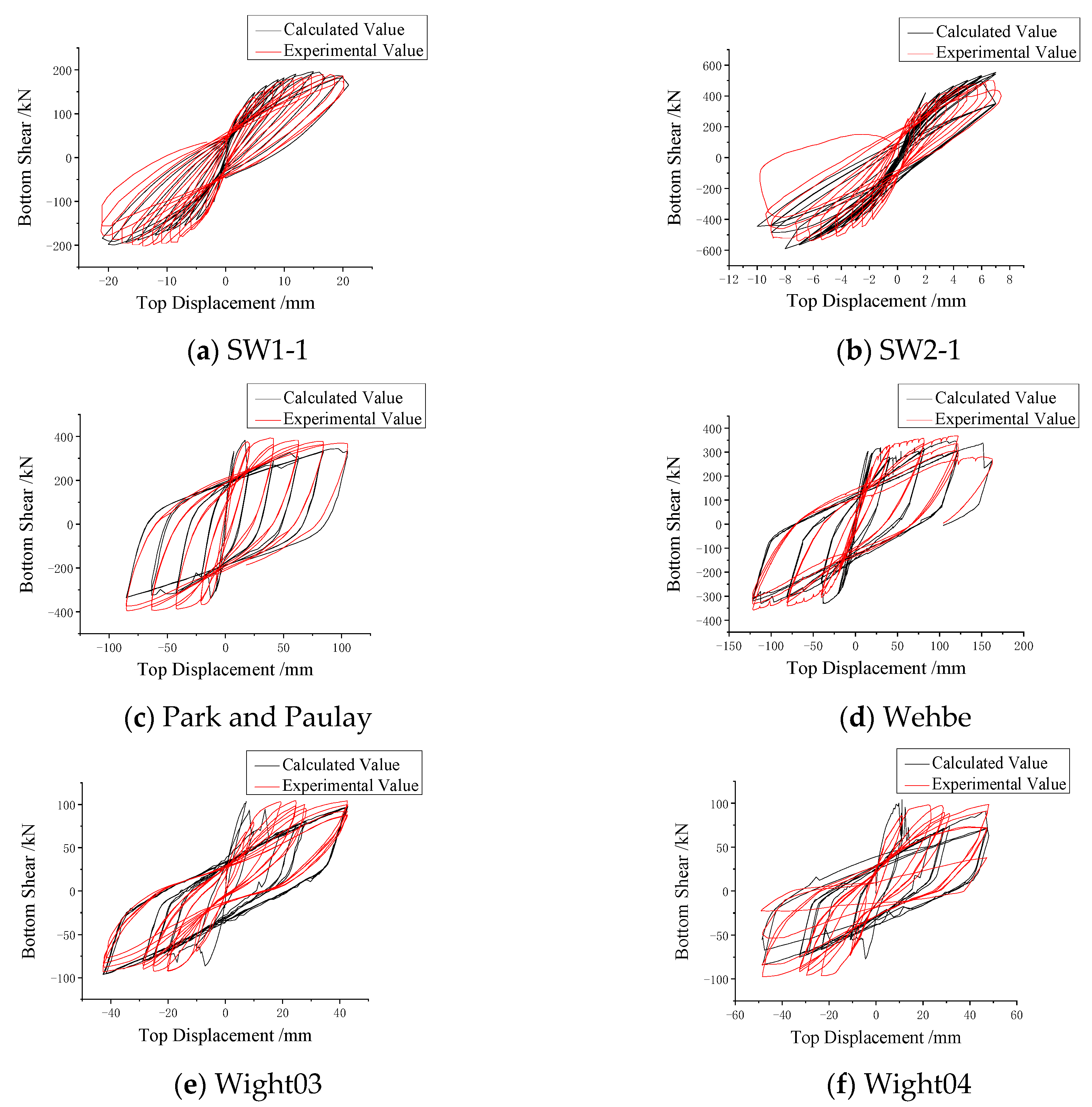
3.2. Probabilistic in-Plane Capability Model of Wall Piers

Based on the statistical investigation of the wall pier girder bridges, the ranges of the parameters are determined and their levels are divided, as shown in

Table 4. Factor levels of wall pier.

Level	1	2	3	4
Aspect ratio	3.2	3.8	4.4	5
Pier width (m)	4	5.33	6.67	8
Vertical reinforcement ratio (%)	0.5	0.63	0.77	0.9
Lateral reinforcement ratio (%)	0.2	0.27	0.33	0.4
Axial pressure ratio	0.02	0.04	0.06	0.08
Shear span ratio	1.6	2.07	2.53	3
Reinforcement grade	HRB400	HRB335	—	—
Concrete marking	C40	C35	—	—

. Orthogonal experimental design is conducted by considering width-to-thickness ratio, pier width, vertical reinforcement ratio, transverse reinforcement ratio, reinforcement grade and concrete strength grade, which results in 16 combinations. A total of 256 wall piers samples were obtained by combining 16 combinations with 4-levels-all-factors combinations of axial compression ratio and shear span ratio. The finite element model of each wall pier is established by employing the layered shell element, and hysteresis analyses are carried out respectively to extract the displacement drift ratio of each sample at each performance limit point. Figure 4 describes the loading path of hysteresis analyses. Each displacement amplitude during loading, which is non-linearly increasing, is cyclically applied twice. The displacement amplitude relationship between $i$ and $i+1$ is $a_{i+1}=1.4a_i$.

After obtaining the displacement drift ratio of each performance limit point, probabilistic capability models of the wall piers can be obtained by statistical regression. Bayesian method has been widely used in the structural capability models due to its iterative ability and high efficiency in parameter stepwise screening [19,20]. Therefore, Bayesian method is utilized to obtain the probabilistic capability models in this study. The basic formula of Bayesian method is as follows:

$$\pi (\theta |x)=\frac{h(x,\theta )}{m(x)}=\frac{f(x|\theta )\pi (\theta )}{{\displaystyle \underset{\Theta }{\int }f(x|\theta )\pi (\theta )d\theta }}$$

(2)

The Bayesian statistical method not only utilizes the overall information and sample information but also utilizes some unknown parameters’ information that has been known before sampling. After obtaining sample $x$ in a sampling, the posterior distribution of the unknown parameter $\theta$ is the conditional distribution of $\theta$ given $X=x$, where $\pi (\theta )$ is the prior distribution of $\theta$, that is, the knowledge of the possible value of the parameter $\theta$ before obtaining the sample $x$, and $m\left(x\right)$ is the marginal distribution of $X$.

In this study, referred to the previous researches on capability models [21], the following probabilistic capability benchmark model is selected after considering the influence of various factors:

$$\begin{array}{l}\ln (\delta )={\alpha }_0+{\alpha }_1\ln (n)+{\alpha }_2\ln (d)\\ +{\alpha }_3\ln (\lambda )+{\alpha }_4\ln (\frac{{\rho }_l{f}_y}{f_c})+{\alpha }_5\ln (\frac{{\rho }_h{f}_y}{f_c})\\ +{\alpha }_6\ln (\frac{f_y}{f_c})+{\alpha }_7\ln ({\rho }_l)+{\alpha }_8\ln ({\rho }_h)+\epsilon \sigma \end{array}$$

(3)

where, $\delta$ is the structural drift ratio, $n$ is the axial compression ratio, $d$ is the width-to-thickness ratio, $\lambda$ is the shear span ratio, ${\rho }_l$ is the vertical reinforcement ratio, ${\rho }_h$ is the transverse reinforcement ratio, $f_y$ is the yield strength of the steel, $f_c$ is the compressive strength of concrete, $\alpha$ is the unknown parameters, $\epsilon$ is the random variable of standard normal distribution, $\sigma$ is the standard deviation of the model error.

Without prior knowledge of the unknown parameters $\alpha$ and $\sigma$, non-information prior was selected as its prior distribution [16]. Assuming that $\alpha$ and $\sigma$ are approximately independent of each other, i.e.,:

$$p(\Theta )\approx p(\alpha )p(\sigma ),\Theta =(\alpha ,\sigma ),$$

(4)

where the prior distribution of parameters $\alpha$ is assumed to be a normal distribution $p(\alpha )\sim N({\mu }_{\alpha },{\sigma }_{\alpha }^2)$, the hyper-parameters ${\mu }_{\alpha }$ values 0 and ${\sigma }_{\alpha }^2$ values ${10}^3$. The prior distribution of $\sigma$ is set as an inverse gamma distribution $\sigma \sim IG(b,c)$, and the hyper-parameters $b$ and $c$ are both set as 0.001 to ensure prior non-information. According to the simulation method in Section 3.2, the hysteretic analysis of 256 wall pier samples is carried out, and the displacement drift ratio of each sample at each performance boundary point is extracted. Based on the structural parameters of the samples and the displacement drift ratios of the performance boundary points, the posterior estimates of the unknown parameters in the probabilistic capability models are obtained by using the Markov chain Monte Carlo (MCMC) method and the statistical software WinBUGS.

The proposed capability model is quite complicated due to the large number of factors considered, and the parameter screening can be efficiently implemented based on the backward stepwise method [19] to achieve a revised formula and to find the parameters that have the most significant impact on the capability model. After obtaining the posterior mean of each unknown parameter, the variation coefficient of each parameter is calculated, and the unknown parameters with a significant coefficient of variation are gradually eliminated. The change of $\sigma$ in the capability model was observed, and the removal stopped when $\sigma$ significantly increased. The specific elimination processes are shown in Figure 5.

Figure 5a–d describe the process of parameter elimination of the probabilistic capacity models at the cracking point, yield point, peak point and limit point, respectively. The abscissa of graphs is the parameter elimination step, and the ordinate is the natural logarithmic variation coefficient of unknown parameters and the natural logarithmic standard deviation. The reason why logarithmize the calculated results is that there are vast differences among the variation coefficients of different parameters.

Taking the process of eliminating the cracking points’ parameters as an example, after obtaining the variation coefficient and the standard deviation by using the sample information and Bayesian method, the variation coefficient of the parameter $a_5$ is founded to be the largest by comparison, thus parameter $a_5$ is eliminated in the first parameter elimination. Similarly, the parameters ${\alpha }_6$, ${\alpha }_2$, ${\alpha }_4$, ${\alpha }_8$ and ${\alpha }_7$ are removed one by one. Whereas when the parameter ${\alpha }_1$ was removed, the standard deviation was significantly increased, that is, the unknown parameter ${\alpha }_1$ could not be removed. The probabilistic capability model of the cracking point is as follows:

$$\delta =e^{-3.047}{n}^{0.264}{\lambda }^{0.637},$$

(5)

where R² = 0.954, standard deviation: $\sigma =0.044$. We use the same method to obtain the probabilistic capability models of the yield point, peak point, and limit point in turn, as shown in Equations (6)–(8):

$$\delta =e^{-1.919}{n}^{0.213}{\lambda }^{0.465}{\rho }_l{}^{0.829},$$

(6)

$$\delta =e^{-2.09}{n}^{-0.332}{\lambda }^{0.71},$$

(7)

$$\delta =e^{-2.067}{n}^{-0.368}{\lambda }^{0.691},$$

(8)

where, yield point $R^2=0.743$; standard deviation $\sigma =0.141$; peak point $R^2=0.636$; standard deviation $\sigma =0.181$; limit point $R^2=0.677$; standard deviation $\sigma =0.173$.

4. Seismic Vulnerability of Wall Pier Girder Bridges

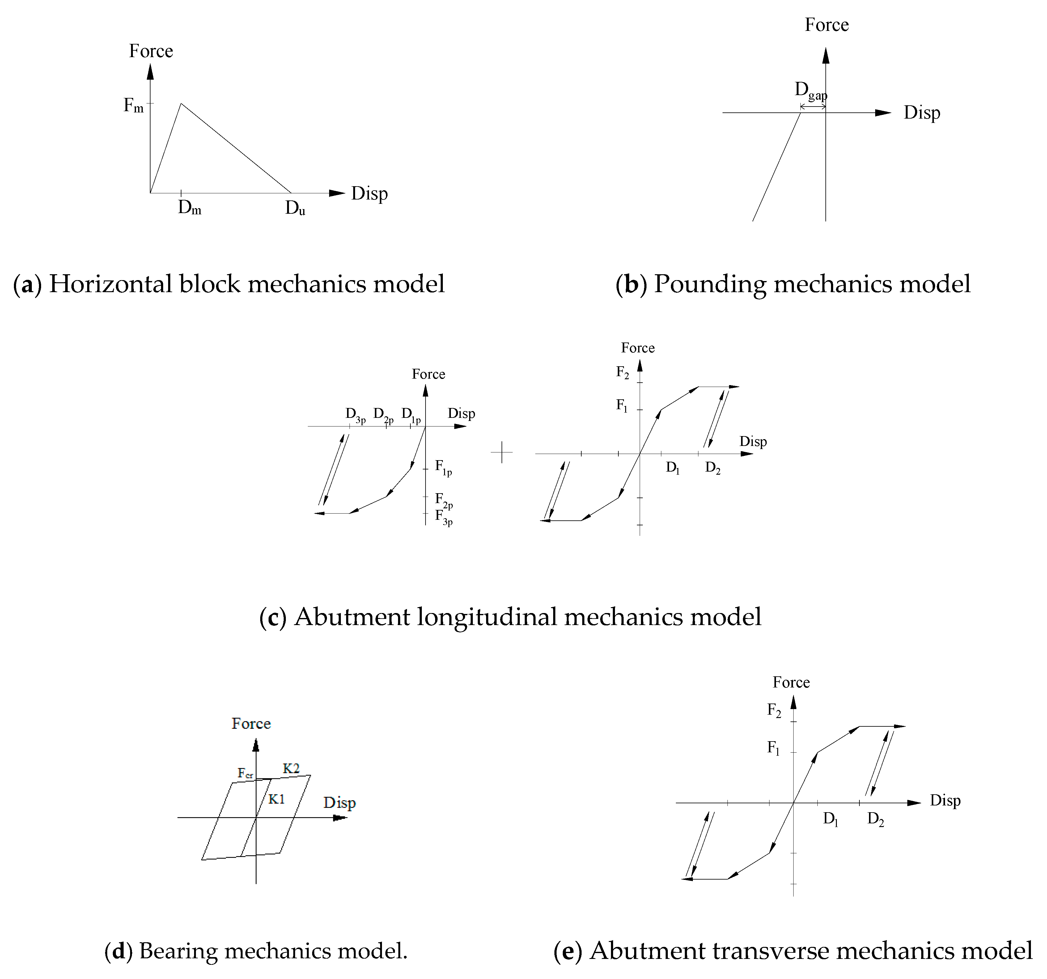
4.1. Bearing and Abutment Limit States

The bearings considered in this study are plate rubber bearing. By referring to the Japanese code [22] and the research of Zhang et al. [23], this study adopts shear strain as the damage index of the bearings. Damage states can be classified as

Table 5. Division of damage states of the bearings.

Performance Level	Damage State	Allowable Quantification of Shear Strain
level Ⅰ	intact	γα < 100%
level Ⅱ	minor damage	100% ≤ γα < 150%
level Ⅲ	medium damage	150% ≤ γα < 200%
level Ⅳ	serious damage	200% ≤ γα < 250%
level Ⅴ	complete destruction	γα ≥ 250%

shows. Because there are few studies available on the damage states of abutments, the performance level is classified as

Table 6. Division of damage states of the abutments.

Performance Level	Damage State	Abutment Limit Displacement Quantification (mm)
level Ⅰ	intact	Δ < 25
level Ⅱ	minor damage	25 ≤ Δ < 50
level Ⅲ	medium damage	50 ≤ Δ < 100
level Ⅳ	serious damage	100 ≤ Δ < 150
level Ⅴ	complete destruction	Δ ≥ 150

by referring to the criterion proposed in HAZUS(2003) [17].

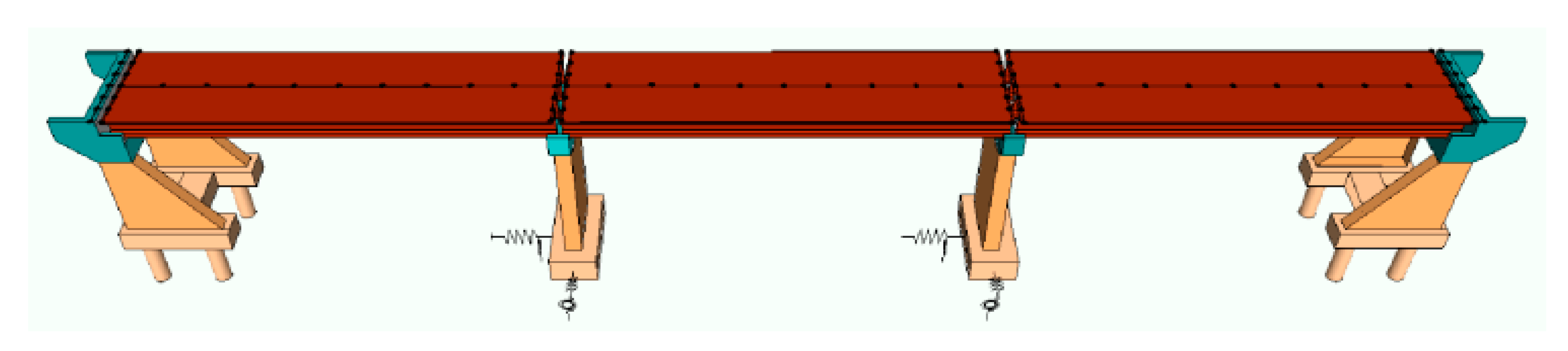
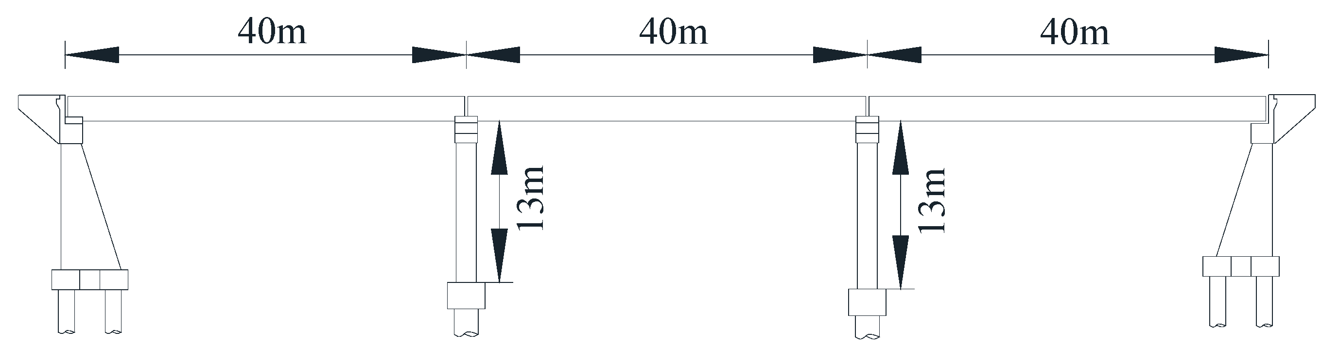
4.2. Bridge Sample Establishment

A three-span prestressed simply supported T-girder bridge is selected as a reference bridge. Each span is 40 m. Its main girder is made of five T-beams, and each T-beam is 2.5 m high and the concrete is C50. The piers, constructed of C35 concrete, are wall piers with a height of 13.5 m, a width of 6.5 m, and a thickness of 1.4 m. HRB335 reinforcements with a diameter of 25 mm are used for pier reinforcements, with a vertical reinforcement ratio of 0.7% and a transverse reinforcement ratio of 0.3%. The capping beams are 10.4 m long, 1 m high and 1.8 m thick, made of C35 concrete. The abutments are pile-supported with bored cast-in-place piles whose diameter is 1.8 m and length is 20 m, and the pile bottom is embedded in sandstone. The elevation layout of the bridge is shown in Figure 6.

In the analysis of probabilistic seismic demand, the uncertainty of parameters should be fully considered. Based on the reference bridge and the researches of previous scholars, the geometric parameters of the bridge, the material parameters and the uncertainty of the parameters in numerical models are taken into consideration in this study.

Table 7. Uncertainty parameter distribution.

Uncertainty Parameter	Distribution Type	Distribution Parameter
		α	β
C35 concrete compressive strength (MPa)	normal distribution	35	4.5
HRB335 steel yield strength (MPa)	logarithmic normal distribution	5.81	0.1
abutment initial stiffness (kN/mm/m)	uniform distribution	11.5	28.5
Scale factor of horizontal resistance coefficient (kN/m4)	uniform distribution	60000	100000
damping ratio	normal distribution	0.045	0.0125
vertical reinforcement ratio of piers (%)	uniform distribution	0.55	0.85
transverse reinforcement ratio (%)	uniform distribution	0.2	0.4
pier height (m)	uniform distribution	11	16
expansion joint width (cm)	normal distribution	8	0.5
shear elastic modulus (MPa)	normal distribution	1.18	0.16

Note: For the distribution parameters α and β, when the distribution type of model parameters is normal distribution, they are mean and standard deviation of the normal distribution respectively, and when the distribution type of the model parameters is uniform distribution, they are the upper and lower bounds of the uniform distribution respectively. When the distribution type of the model parameters is logarithmic normal distribution, the parameters α and β are numerically equal to the logarithmic mean and standard deviation.

lists the random parameters and their probability distributions. Latin hypercube sampling is used for each parameter to obtain 120 samples, and 120 bridge samples can be obtained by randomly combining the values of geometric parameters and material parameters.

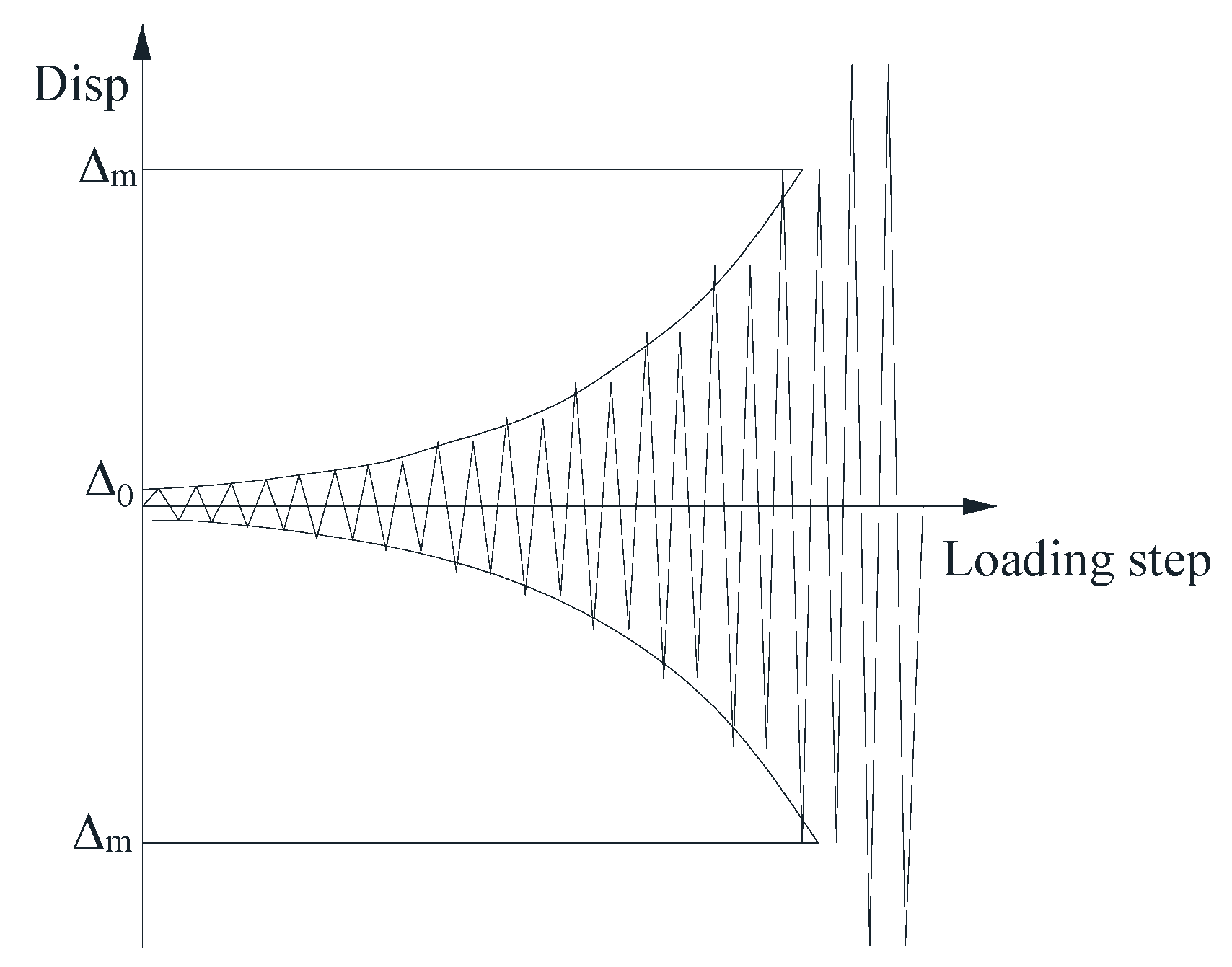
4.3. Time-History Analysis

OpenSees is used for the analysis. The main girder is simulated by three-dimensional elasticBeamColumn elements. The bearings are simulated by flatSliderBearing elements and their sliding effects are considered. The foundations are simulated by EqualDOF mode, and the stiffness of each direction is calculated according to the specification. Simplified models of the abutments are established by referring to California code for seismic design of bridges [24], and their mechanical effects are calculated. The transverse and longitudinal restraint effects of pile foundations on abutment are considered by referring to Nielson’s research [25]; according to the research of Xu Lueqin et al [26], simplified mechanical models are adopted for the baffle block, without considering the pounding effect between the main girder and the block. The pounding effects between the main girders, as well as between the main girder and the abutment, are simulated by linear springs, and the pounding stiffness are calculated after referring to the research of Xia Qi et al. [27]. The corresponding finite element models of 120 bridge samples were built. The entire bridge model and the mechanical models of each component are shown in Figure 7 and Figure 8 below:

Twenty near-field and far-field ground motions are selected from the database of Pacific Earthquake Engineering Research Center of the United States. The selection criteria are shown in

Table 8. Ground motion selection criteria.

Type of Ground Motions	Types	Fault Distance (R)	Intensity Magnitude	PGV/PGA
near field	pulse type	0~20km	6~8	>0.15
far field	non-pulse type	20~100km	6~8	≤0.15

. PGA is used as the intensity measure (IM) of the ground motions, and the ground motions are corrected and cut off respectively. According to the IM, 40 ground motions are modulated to 1.0, 1.5 and 2.0 times respectively, thus 120 ground motions are obtained. The ground motions and the bridge samples are matched one by one for time-history analysis, then the seismic demand of each vulnerable component is obtained.

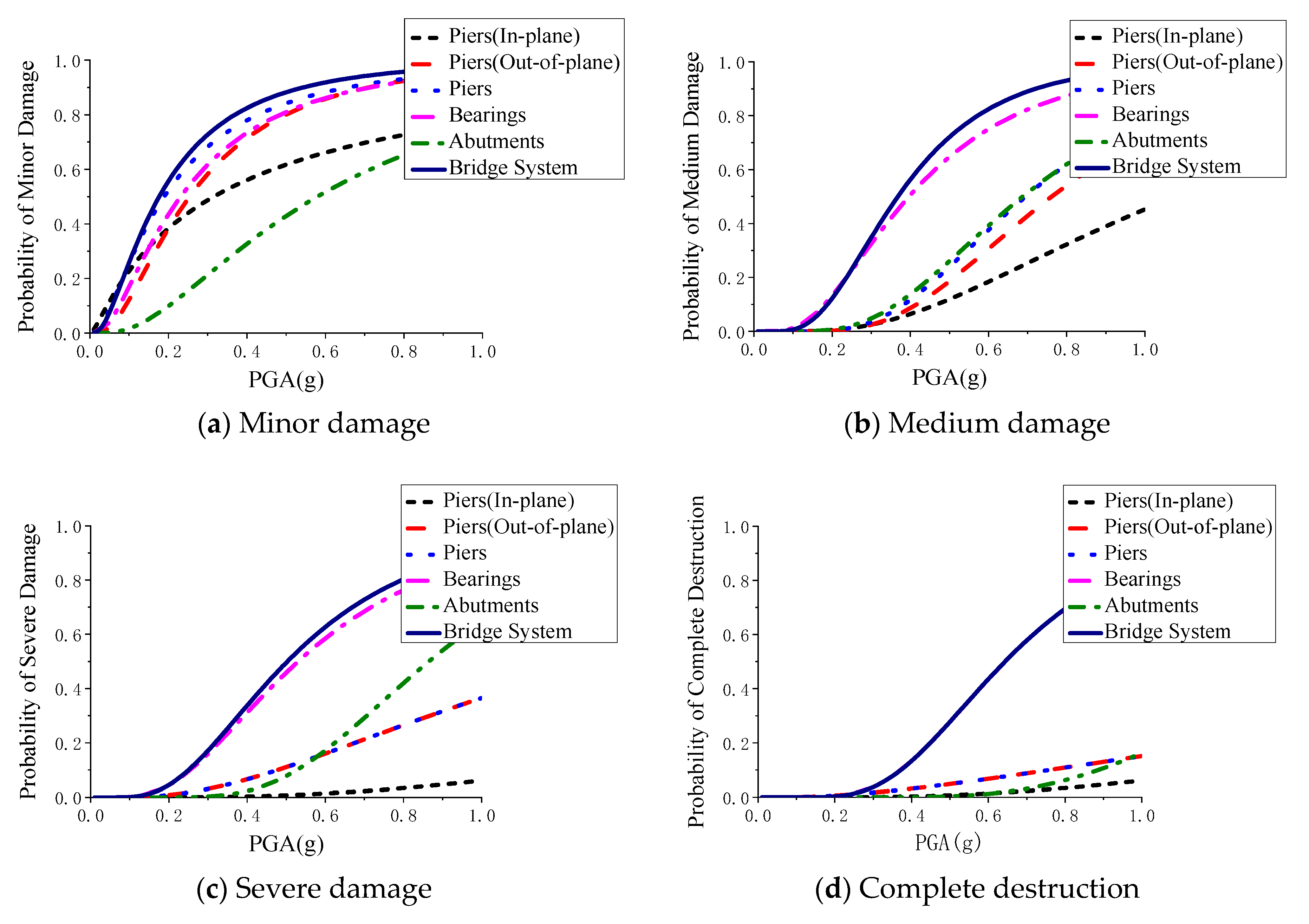
4.4. Seismic Vulnerability of Wall Pier Bridges

Seismic vulnerability is generally defined as the probability that a component or structure will reach a specific damage state at a given ground motion intensity measure IM. The specific expression is $P[D\ge C|IM]$, where, $C$ denotes the seismic capacity and is a property of the structure itself; $D$ denotes the earthquake demand, which is obtained through the dynamic time-history analysis and is related to the ground motion intensity. It is assumed that the seismic fragility models of the wall pier bridge and its components follow a logarithmic normal distribution, as shown by the following equation:

$$P\left[D\ge C|IM\right]=\Phi \left[\frac{\ln \left(IM\right)-\ln \left(m\right)}{\beta }\right]$$

(9)

where m and $\beta$ denote the median value and logarithmic standard deviation of the seismic vulnerability mode respectively l. Meanwhile, the bridge system is regarded as a series system to obtain the seismic fragility parameters m and $\beta$ of the vulnerable components and the bridge system by maximum likelihood estimation. The specific calculation results are shown in

Table 9. The median and logarithmic standard deviation in the fragility models of bridge components and bridge systems to different damage states.

Component	Minor Damage		Medium Damage		Severe Damage		Complete Destruction
	Median Value (g)	Logarithmic Standard Deviation	Median Value (g)	Logarithmic Standard Deviation	Median Value (g)	Logarithmic Standard Deviation	Median value (g)	Logarithmic Standard Deviation
Pier (out of plane)	0.2541	0.8003	0.7618	0.4712	1.3108	0.7875	3.1159	1.1027
Pier (in plane)	0.316	1.5414	1.0808	0.6534	3.3743	0.7875	3.3743	0.7875
Pier (overall)	0.1892	0.9701	0.695	0.463	1.3108	0.7875	3.1159	1.1027
Bearing	0.2312	0.8775	0.3966	0.6135	0.5306	0.5739	0.6435	0.4278
Abutment	0.5759	0.8253	0.6877	0.4962	0.8648	0.3866	1.4911	0.4057
Bridge system	0.1767	0.8758	0.3682	0.5241	0.5031	0.5449	0.6435	0.4278

. The fragility curves of different components and bridge system are shown in Figure 9 below:

It can be seen from Figure 9a that the damage probabilities of the piers under various ground motion intensities are higher than that of the bearings and the abutments. When the ground motion intensity is less than 0.16 g, the damage probability of the piers in transverse direction is higher than that of the pier in out-of-plane direction, the bearing and the abutment. The main reason is that the tensile strength of concrete is low and cracks are likely to appear under the action of ground motions. It can be seen from Figure 9b that under various ground motion intensities, the damage probability of the bearings is higher than that of other components and the in-plane damage probability of the pier is the lowest. The rule of the damage probability of each component in Figure 9c is similar to that of Figure 9b. It can be inferred from Figure 9d that when the ground motion intensity is higher than 0.3 g, the damage probability of the bearings and of the bridge system increases rapidly with the increase of the ground motion intensity, while the damage probability of other components increases slowly.

Based on the four graphs (a) to (d) in Figure 9, it can be found that the wall piers perform well under the action of earthquake, and the wall piers have the lowest damage probability in the medium damage state, severe damage state and complete destruction state. The statistical parameters of the in-plane vulnerability curve in severe damage state and the complete destruction state are the same, and the primary reason is that the in-plane bearing capacities of the structures is rapidly decreased after the wall piers reach a serious damage state, and the structures quickly enter the complete destruction state. In the medium damage state, severe damage state and complete destruction state, the vulnerability curve of the bridge system and the bearings are closest or coincident, that is, their seismic vulnerabilities are closely related.

5. Conclusions

A study is carried out on wall pier girder bridges. Finite element models of the wall piers are established by the layered shell element and their accuracy is verified. Hysteresis analyses of the wall pier samples are carried out to obtain the drift ratio at each performance limit point. The Bayesian method is used to obtain the probabilistic in-plane performance model of the wall piers. Finite element models of the wall pier girder bridges are further established and the seismic vulnerabilities of wall pier girder bridges and their components are obtained by time-history analysis. The main conclusions are as follows:

(1) By comparing the finite element simulation methods of the common pier columns and shear wall structures, the layered shell element is selected to carry out finite element analyses of the wall piers, and its accuracy is verified. When compared to other cases, it is found that the finite element analysis of components with small aspect ratio will cause a sharp drop in bearing capacity when the layered shell element is used, but in general the layered shell element can well simulate the different failure modes and mechanical properties of the components.

(2) The displacement drift ratio at each performance limit point of 256 wall pier samples is obtained by numerical analysis. The Bayesian method is used to estimate and eliminate the unknown parameters in the proposed probabilistic capacity models of the wall piers. It can be seen from the probabilistic capacity models that the displacement drift ratio at each performance state limit point is mainly related to the axial compression ratio, the shear span ratio and the vertical reinforcement ratio. The displacement drift ratios of the components are positively correlated with the axial compression ratio when the components are cracked or yielded, negatively correlated with the axial compression ratio when the bearing capacities reach the peak or the limit state, and the displacement drift ratios of the components at the limit point of each damage state are all positively correlated with the shear span ratio.

(3) Based on a reference bridge, 120 bridge samples are generated considering the uncertainty of parameters, and the seismic vulnerability model parameters of bridge components and bridge systems are obtained by time-history analysis. The seismic vulnerability analysis results of each component and bridge system show that the damage probabilities of the wall piers are the highest in the minor damage state and the damage probabilities of the bearings are the highest in other states. The wall piers are easy to enter the complete destruction state after they enter the serious damage state due to the decrease of bearing capacity. Generally, the wall pier structures perform well under the action of ground motions, and the bearings have a significant influence on the seismic vulnerability of the bridge system.

References

1. Bignell, J.L. Assessment of the Seismic Vulnerability of Wall Pier Supported Highway Bridges on Priority Emergency Routes in Southern Illinois. Ph.D. Dissertation, University of Illinois at Urbana-Champaign, Urbana, IL, USA, 2006. [Google Scholar]
2. Bayat, M.; Daneshjoo, F.; Nistico, N. Probabilistic sensitivity analysis of multi-span highway bridges. Steel Compos. Struct. 2015, 1, 237–262. [Google Scholar] [CrossRef]
3. Haroun, M.A.; Pardoen, G.C.; Shepherd, R.; Haggag, H.A.; Kazanjy, R.P. Cyclic Behavior of Bridge Pier Walls for Retrofit; University of California Irvine: Irvine, CA, USA, 1993. [Google Scholar]
4. Aboutaha, R.S.; Engelhardt, M.D.; Jirsa, J.O.; Kreger, M.E. Rehabilitation of shear critical concrete columns by use of rectangular steel jackets. ACI Struct. J. 1999, 96, 68–78. [Google Scholar]
5. Greifenhagen, C. Seismic Behavior of Lightly Reinforced Concrete Squat Shear Walls. Ph.D. Dissertation, Dresden University of Technology, Dresden, Germany, 2006. [Google Scholar]
6. Hidalgo, P.A.; Ledezma, C.A.; Jordan, R.M. Seismic Behavior of Squat Reinforced Concrete Shear Walls. Earthq. Spectra 2002, 18, 287–308. [Google Scholar] [CrossRef]
7. Baker, J.W. Efficient analytical fragility function fitting using dynamic structural analysis. Earthq. Spectra 2015, 31, 579–599. [Google Scholar] [CrossRef]
8. Leborgne, M.R. Modeling the Post Shear Failure Behavior of Reinforced Concrete Columns. Ph.D. Dissertation, University of Texas at Austin, Austin, TX, USA, 2012. [Google Scholar]
9. Sun, Z.; Li, H.; Wang, D.; SI, B. Discrimination criterion governing flexural-shear failure modes and improved seismic analysis model for RC bridge piers. China J. Highw. Transp. 2015, 28, 42–50. (In Chinese) [Google Scholar]
10. Zhang, L.; Yang, H. Hysteresis shear models for shear-wall. World Inf. Earthq. Eng. 1999, 15, 9–16. (In Chinese) [Google Scholar]
11. Orakcal, K. Nonlinear Modeling and Analysis of Slender Reinforced Concrete Walls. Ph.D. Dissertation, Department of Civil and Environmental Engineering, University of California Los Angeles, Los Angeles, CA, USA, 2004. [Google Scholar]
12. Orakcal, K.; Conte, J.P.; Wallace, J.W. Flexural Modeling of Reinforced Concrete Structural Walls—Model Attributes. ACI Struct. J. 2004, 101, 688–698. [Google Scholar]
13. Kolozvari, K.; Orakcal, K.; Wallace, J.W. Shear-Flexure Interaction Modeling of Reinforced Concrete Structural Walls and Columns under Reversed Cyclic Loading; Pacific Earthquake Engineering Research Center, University of California Berkeley: Berkeley, CA, USA, 2015; PEER Report No. 2015/12. [Google Scholar]
14. Lu, X. Elasto-Plastic Analysis of Buildings Against Earthquake; China Architecture & Building Press: Beijing, China, 2015; pp. 62–63. (In Chinese) [Google Scholar]
15. Zhang, H. Study on the Performance-based Seismic Design Method for Shear Wall Structures. Ph.D. Dissertation, Tongji University, Shanghai, China, 2007. (In Chinese). [Google Scholar]
16. Berry, M.; Parrish, M.; Eberhard, M. PEER Structural Performance Database User’s Manual; Pacific Earthquake Engineering Research Center, University of California Berkeley: Berkeley, CA, USA, 2004; Available online: https://nisee.berkeley.edu/spd/ (accessed on 31 December 2019).
17. FEWA; HAZUS-MH MR4. Technical Manual: Earthquake Model; Federal Emergency Management Agency: Washington, DC, USA, 2003. [Google Scholar]
18. Sun, Y.; Zhuo, W.; Fang, Z. Definition and quantified description of seismic performance levels for regular bridges. J. Earthq. Eng. Eng. Vib. 2011, 31, 104–112. (In Chinese) [Google Scholar]
19. Gardoni, P. Probabilistic Models and Fragility Estimates for Bridge Components and Systems. Ph.D. Dissertation, University of California Berkeley, Berkeley, CA, USA, 2002. [Google Scholar]
20. Gelman, A.; Carlin, J.B.; Stern, H.S.; Dunson, D.B.; Vehtari, A.; Rubin, D.B. Bayesian Data Analysis, 3rd ed.; Chapman and Hall/CRC: New York, NY, USA, 2013. [Google Scholar]
21. Zhu, L.; Elwood, K.J.; Haukaas, T. Classification and Seismic Safety Evaluation of Existing Reinforced Concrete Columns. J. Struct. Eng. 2007, 133, 1316–1330. [Google Scholar] [CrossRef]
22. Japan Road Association. Specifications for Highway Bridges: Part V. Seismic Design; Maruzen: Tokyo, Japan, 2002. [Google Scholar]
23. Zhang, J.; Huo, Y. Evaluating the effectiveness and optimum design of isolation devices for highway bridges using the fragility function method. Eng. Struct. 2009, 31, 1648–1660. [Google Scholar] [CrossRef]
24. California Department of Transportation. Seismic Design Criterial Version 1.7; California Department of Transportation: Sacramento, CA, USA, 2013. [Google Scholar]
25. Nielson, B.G. Analytical Fragility Curves for Highway Bridges in Moderate Seismic Zones. Ph.D. Dissertation, Georgia Institute of Technology, Atlanta, GA, USA, 2005. [Google Scholar]
26. Xu, L.; Li, J. Effect of retainers on transverse seismic response of a standard continuous girder bridge. J. Highw. Transp. Res. Dev. 2013, 30, 53–59. (In Chinese) [Google Scholar]
27. Xia, Q.; Luo, R. Bridge Impact Stiffness Values of Correction in the Earthquake. Open J. Transp. Technol. 2013, 2, 200–205. (In Chinese) [Google Scholar] [CrossRef]
Figure 1. Schematic diagram of layered shell element.
Applsci 10 00926 g001
Figure 2. Comparison between experiment results and finite element simulations.
Applsci 10 00926 g002
Figure 3. Dipiction of the pier damage states.
Applsci 10 00926 g003
Figure 4. Loading process of displacement control.
Applsci 10 00926 g004
Figure 5. Remove the parameters of the performance point.
Applsci 10 00926 g005
Figure 6. Elevation drawing of the benchmark bridge.
Applsci 10 00926 g006
Figure 7. Bridge model.
Applsci 10 00926 g007
Figure 8. Mechanics models of bridge components.
Applsci 10 00926 g008
Figure 9. Seismic fragility curves of the bridges.
Applsci 10 00926 g009