Abstract
The traditional free-space and half-space analysis method ignore the reflection of the upper and lower boundaries of shallow sea and are not suitable for analyzing shallow sea problems especially at high frequency. Hence, a method combining ray theory and wave superposition theory is proposed in this paper to predict the high-frequency radiated acoustic field in shallow water. The proposed method takes into account the effect of channel boundaries on the acoustic field and has good adaptability to complex channel environments and accuracy of the calculated acoustic field.
1. Introduction
The accurate prediction of acoustic radiation of underwater vehicles is an important engineering application. The accurate simulation of radiated noise is also important for acoustic field characteristics analysis and acoustic measurement research. The oceans surrounding China mostly consist of shallow water and have a typical shallow water waveguide environment. In the shallow sea, the traditional free-space analysis method is limited due to the acoustic reflection phenomenon of the upper and lower boundary surfaces, and the acoustic radiation prediction in the shallow sea becomes very complicated.
The acoustic propagation model used in sea includes ray theory [1], normal model theory [2,3], wavenumber integration method [4], and parabolic equation method [5]. The advantage of the ray theory is that the physical meaning is intuitive and has good adaptability to high frequency problems. The normal wave theory is suitable for low frequency problems and provides accurate calculation in the far field. The wave number integration method is an integral transformation method of a horizontal layered medium and provides fast calculation speed. The parabolic equation method performs better in dealing with the problem of sound propagation in the environment related to distance. This kind of research method that uses a point source, ignores the vibration distribution of the structure surface and the directivity of the acoustic radiation. Hence, it is not appropriate to regard the elastic structure as a point source with the same source strength and directivity. The Finite Element Method (FEM) is only applicable to the near field region. However, for the far acoustic field, and with the high frequency condition, the number of grid elements in the FEM is too large to calculate, and the FEM is inapplicable in this scenario. The wave superposition method [6,7] has excellent structural adaptability. Most of the current research focuses on free space and half-free space, but there are few researchers who concentrate on the sea waveguide [8,9,10,11].
For the acoustic radiation problem of the elastic structure in the shallow sea, some combined models are developed under the condition that it is difficult to meet the calculation requirements by a single method. Shang proposed a method that combines the wave superposition method and normal mode Green’s function method, which effectively predicted the acoustic radiation of large elastic structures under shallow sea [12]. This method uses the normal mode Green’s function to calculate the far field pressure, while the normal mode green function has a large order at high frequencies, which has a greater impact on the computational efficiency. Hence, this method is not appropriate for calculation speed at high frequencies. Qian proposed a method that combines the finite element method with the parabolic equation method to obtain cylindrical field data in the near field active region, and a complete far field solution in the far-field passive region, using the parabolic equation method [13]. The parabolic equation method is a recursive method, and far field calculation leads to error accumulation. In addition, it is difficult to directly obtain the data of a near field cylindrical field.
In this paper, a new method is proposed for the prediction of an acoustic field radiated from the structure excited at a frequency. Based on the combination of wave superposition and ray theory, the structure source is equivalent to a set of virtual sources that are reconstructed by matching the surface normal velocity of the structure source. Finally, the complete acoustic field is obtained by superimposing sound radiation fields from all virtual sources using ray theory.
2. Theoretical Model
The proposed theoretical model consists of the combination of wave superposition theory and ray theory, corresponding to the acoustic inverse problem and the acoustic positive problem respectively.
2.1. Wave Superposition Theory
The acoustic field radiated by the elastic structure in the fluid environment meet the Sommerfeld radiation condition in the far field, and the fluid–solid coupling boundary satisfies the condition of the normal vibration velocity. Additional boundary conditions for the Helmholtz equation can be expressed as:
where, is the normal velocity of the fluid medium, and is the normal vibration velocity of the structural surface in the fluid medium. Equation (3) shows the Sommerfeld far field radiation condition. The equation can be solved by the Helmholtz integral formula.
For any shape of radiator, the radiated pressure at the field is the integral of the internal volume source of the structure as shown as:
where, and are coordinates of the field point and virtual source in the global coordinate system, respectively. The shows medium density in field, is the angular frequency, is strength of the virtual source, and is the Green’s function under the corresponding boundary conditions. A schematic diagram is shown in Figure 1.
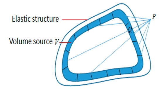
Figure 1.
Schematic diagram of wave superposition theory.
For the typical channel environment (i.e., the sea surface is the Dirichlet boundary and the sea floor is the Neumann boundary), the normal mode Green’s function in cylindrical coordinates can be shown as [14]:
where, shows the source depth, is depth of the sea, and represent the vertical and horizontal components of the wave number , respectively, and is Eigen function with different forms under different boundary conditions. The parameter is the horizontal distance, and is the normal order. Introducing the linear Euler formula to transform Equation (4) into an integral representation of normal vibration velocity on the surface can be expressed as:
where, Equation (6) relates the surface normal velocity to the Green’s function. In theory, there is no limit for the placement of virtual sources and they can be located anywhere within the structure. Related studies have shown that the virtual source surface and the surface of the structure are in the same shape, which can improve the inversion accuracy of the configured equivalent source. It can be assumed that the virtual source is distributed over a virtual spherical shell surface of thickness inside the structure; hence, Equation (6) can be written as:
where is the node coordinate on the surface of the structure. Dividing the virtual spherical shell into parts, each surface of the structure is shown by . If each spherical shell crown is small enough, the summation coefficient can be regarded as constant, and the normal vibration velocity at different points on the structural surface can be approximately written as:
where, represents the coordinate of the ith virtual source, and represents the strength of the ith source on the virtual surface. Hence, Equation (8) can be written in the matrix as:
The structural surface normal velocity matrix in Equation (9) can be expressed by the source strength matrix and transfer matrix , where can be expressed as:
It should be noted that in practical applications, the matrix may be an ill-conditioned matrix, and slight disturbance of vibration velocity will cause a dramatic change in virtual source strength. According to the acoustic inverse problem observed in a literature study, the Tikhonov regularization method based on L curve can effectively suppress the disturbance and effectively deal with the ill-conditioned matrix before solving the inverse problem [15]. For the same discrete processing method in Equation (4), the pressure at point can be expressed as the superposition of discrete point source radiated acoustic fields as shown as:
2.2. Ray Theory
The ray solution exists in the form . Where represents the wave number at the initial position, is the sound speed of the initial position, is the index of refraction, and is the wave number at position . The represents the pressure amplitude and shows the pressure phase. Substituting the ray solution into the wave equation, the following two equations can be obtained as [16]:
When is much smaller than , then
In ray theory, Equations (14) and (15) are called as eikonal equation and intensity equation respectively, and are the two basic equations of ray theory [17]. In ray theory, the propagation of waves are usually regarded as the propagation of an infinite number of acoustic rays. Each ray is perpendicular to the equiphase surface, and the propagation path in the sea is affected due to the medium and boundary. The sound ray carries energy, and the energy in each sound ray does not lose to the outside of the sound ray. These sound rays contribute to the acoustic field in ray theory.
Eikonal equation combined with Snell’s law, to obtain the trajectory of the ray, satisfies the following relationship [18] as shown below:
After giving the initial glancing angle and the sound speed function , the solution of the above equation can achieve ray tracking and acquire ray trajectories. The eigenray are determined in the distribution trend of the rays, which are special rays that directly supply the power at a certain point in the acoustic field. The energy of each sound ray can be derived from the intensity equation as:
where represents the radiated power in unit solid angle. The energy of these rays reflects due to the boundary and distributes in the acoustic field in a steady state. After determining the position and strength of virtual sources by wave superposition method, the acoustic field is calculated by ray theory. Then the prediction of the structured radiation acoustic field is realized.
3. Accuracy Analysis of Combined Wave Superposition Method
The combined wave superposition method (combined WSM) is an approximation method, and the accuracy of the approximation is needed to be discussed. It approximates not only the normal mode order of the Green’s function in sea, but also the process of inverting the virtual source strength. The ray theory is also an approximate acoustic propagation model in the acoustic positive problem. In the following sections, we will analyze the error caused by the local approximation in combined WSM, and some characteristics of the whole method in numerical calculation.
3.1. Accuracy Analysis of Green’s Function in Channel
The basis of the wave superposition method is the Green’s function. The accuracy of the Green’s function, especially in the near field, directly determines the accuracy of the transfer matrix. The Green’s function is expressed as the sum of the normal modes. The high-order normal mode has little contribution to the far field; however, it has a great influence on the near field. Therefore, the normal order determines the near field accuracy of the Green’s function. When the order is too small, the result of the Green’s function is inaccurate in the near field, but gradually approaches the exact value as the distance increases.
In order to illustrate the near field accuracy of the Green’s function, a case is selected for analysis. In the shallow sea of 200 m depth, the sea surface is the Dirichlet boundary and the sea floor is the Neumann boundary. A point source with a frequency of 20 Hz is located at a depth of 25 m. According to the boundary conditions, the following constraints exist in Equation (5) as shown as:
The eigen function that satisfies the constraints is . The specific form of the Green function can be obtained according to the constraint conditions, which is the analytical solution under boundary condition as shown as:
where, shows the source depth, indicates the depth of the sea, and and represent the vertical and horizontal components of the wave number , respectively. The parameter is the horizontal distance, and is the normal order.
The model is built using finite element software COMSOL and compared with the Green’s function method when the mesh density is sufficiently dense, and the results are shown in Figure 2.
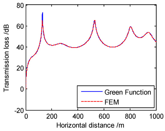
Figure 2.
Comparison of far field transmission loss between Green’s function method and finite element method.
It can be seen that under far field conditions, the calculation result of the Green’s function is nearly consistent with the finite element method. In fact, the situation is different under near field conditions, which is what needs to be discussed next.
We assume the error threshold 1 dB, that is, the accuracy of the near field calculation is characterized by the horizontal distance when the absolute error between the transmission loss of the Green’s function method and the finite element method is less than 1 dB. The further the distance is, the more accurate are the results of the near field of the Green’s function we obtain. Figure 3 below shows the near field accuracy of the Green’s function after changing the normal mode order of the Green’s function at different frequencies or different depths, while the sea environment and point source parameters are consistent with the above case.
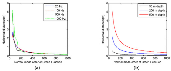
Figure 3.
The near field accuracy of the Green’s function at different frequencies or different depths. (a) Accuracy of different frequencies at a depth of 200 m; (b) Accuracy of different depths at a frequency of 20 Hz.
The overall trend is that if the order is larger, the results of the near field of the Green’s function are more accurate. In order to ensure that the wave superposition method can effectively reverse the acoustic field information, it needs to increase the order and to ensure that the horizontal distances from the equivalent sources to the positions of vibration velocity point are not too close. As the frequency increases, the energy of the acoustic field concentrates on the low-order normal modes, and loss due to the lack of energy of the high-order is also reduced. However, in order to get the accuracy of the near-field, it is necessary to keep the order large enough. In terms of greater depth, the requirement of the normal order is higher in this method. Therefore, theoretically the accuracy of the wave superposition method can be guaranteed with a small depth.
3.2. Applicability of Rays Superimposed
For the Green’s function requiring high-order superposition, the calculation time of each virtual source propagating the acoustic field increases rapidly with the increase of the calculated range and order, making the calculation efficiency low. The large number of virtual sources inversion by the wave superposition method makes the superposition with the Green’s function not the most ideal choice. The ray theory performs ray tracing in the entire acoustic field and extracts the eigenray, which is less computationally expensive. Since the ray theory is derived under the high frequency approximation, it is necessary to verify that the ray solution can meet the accuracy requirements of the acoustic field superposition at different frequencies and depths.
The channel is a typical shallow sea waveguide (i.e., the sea surface boundary is the Dirichlet boundary; the sea bottom boundary is the Neumann boundary), and the six point sources are located at depths of 25 to 30 m at intervals of 1 m. The depth of water and frequency are changed, and the acoustic field is superimposed by the ray theory and the Green’s function method, respectively. The field comparison chart after superposition is shown in Figure 4 as:
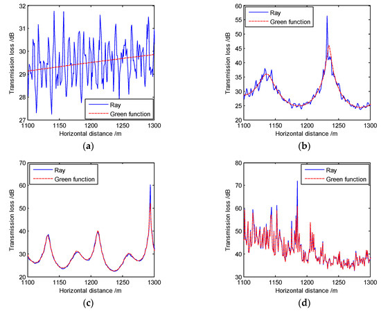
Figure 4.
The field comparison chart after superposition at different frequencies and depths. (a) Comparison at 20 Hz and 50 m; (b) Comparison at 50 Hz and 50 m; (c) Comparison at 50 Hz and 100 m; (d) Comparison at 1000 Hz and 50 m.
The ray solution will have a slight oscillation near the true value at low frequency, and the superposition of multiple point sources will amplify the amplitude of the oscillation. A large number of virtual sources can cause an increase in the amplitude of the oscillation. The amplitude of the oscillations is different at different frequencies and depths. The error caused by oscillation is characterized by mean square error (MSE).
where represents the number of measurement points, and and are the transmission losses obtained by ray theory and the Green’s function methods respectively. The table below gives the MSE for certain frequencies and depths.
In Table 1, in the case where the frequency is too low or the depth is too small, there is a large error in ray theory. At high frequency, the solution of the ray theory is very accurate. The field of virtual source can be directly superimposed, and the result is reliable. As a whole, the oscillation of the ray theory has a limited influence on the calculation results. The performance at high frequency is superior, and the application range of the wave superposition method can be expanded.

Table 1.
MSE of the solution of the ray solution compared to the Green’s function for different frequencies and different sea depths.
3.3. Calculation of Acoustic Radiation Field by Combined Method
The key to the combined method is the solution of the acoustic inverse problem. The results of the virtual source inversion have a significant impact on the calculation of the acoustic field [19]. Research shows that the accuracy of wave superposition inversion has a great relationship with virtual source configuration. These researches are based on free space or half space Green’s function, but the Green’s function in sea is a cylinder functions, which has its own particularity. In order to illustrate the calculation accuracy of the method proposed in this paper and analyze the influence of different virtual source configuration methods, an excited spherical shell is selected to calculate its far field pressure using the proposed method and compared with the finite element model in COMSOL software. The reason why this axisymmetric structure was selected is that the calculation distance of the three-dimensional field by COMSOL is limited by the performance of the computer. The selected spherical shell has a radius of 2 m and a thickness of 0.1 m. The Material elastic Young’s modulus is and Poisson’s ratio is ; density is . The outside medium is water, in which the density is , and the speed of sound is . The inside of the spherical shell is a vacuum. The center of the spherical shell is located at a water depth of 25 m. A normal force of 1 N with a frequency of 100 Hz is applied at the bottom of the spherical shell. The depth of the sea is 200 m, and the sea surface and seabed boundary conditions satisfy typical channel conditions. The schematic diagram of the COMSOL model is shown in Figure 5. The sound pressure level (SPL) of the radiated field of this model is calculated using COMSOL. As the spherical shell is circumferentially symmetrical, the vibration velocity of the two-dimensional structure surface calculated by COMSOL can be scanned every 36 degrees in the circumferential direction to obtain the three-dimensional structure surface vibration velocity distribution. We also calculate SPL of the radiated field using combined WSM based on 3D vibration velocity distribution data.
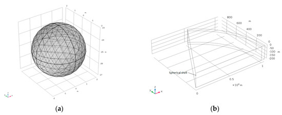
Figure 5.
The schematic diagram of the COMSOL model. (a) The schematic diagram of the spherical shell in COMSOL; (b) The schematic diagram of the sea channel in COMSOL.
The virtual sources are distributed on a surface that has the same shape as the surface of the structure, which is an appropriate virtual source configuration. The virtual source surface is generally obtained by shrinking the surface of the structure inwardly. Here the radius ratio is chosen to be 0.5. Except for the upper and lower vertices, the virtual source surface is divided into 10 and 6 intervals in the circumferential and vertical directions respectively, that is, a total of 72 virtual source points ( virtual sources) are created, as shown in Figure 6.
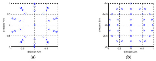
Figure 6.
Schematic diagram of virtual source placement (virtual sources); (a) Top view; (b) Front view.
The sound pressure level is calculated at different depths as shown in Figure 7.
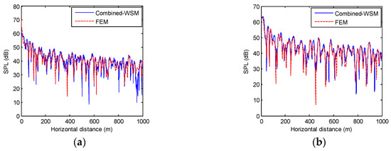
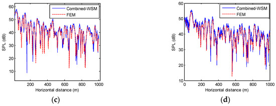
Figure 7.
The SPL at the depth of 25 m and 50 m (100 Hz). (a) The depth of 25 m; (b) The depth of 50 m; (c) The depth of 100 m; (d) The depth of 150 m.
The SPL is calculated at the received depth of 25 m, 50 m, 100 m, and 150 m. The results of combined WSM are compared with the finite element calculation results. Further, the relative error is defined as:
where, is the number of measurement points. The and are the sound pressures generated by combined WSM and FEM, at the ith measurement point, respectively. The and virtual sources (excluding the upper and lower vertices) are selected respectively, to form a virtual source surface, as shown in Figure 8, and analyzed the effect of the radius ratio on the calculation result at the receive depth of 25 m, as shown in Figure 9.
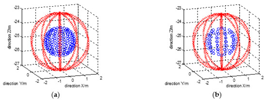
Figure 8.
Different virtual source surface. (a) Virtual sources; (b) Virtual sources.
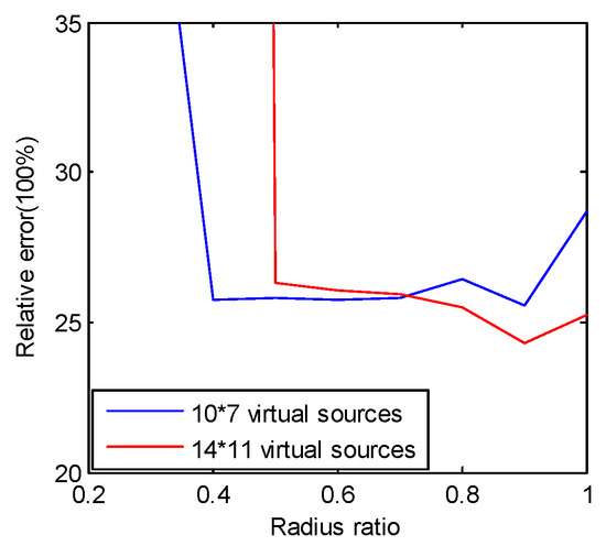
Figure 9.
The effect of radius ratio and the number of virtual sources on the calculation result.
Theoretically, when the number of virtual sources is large, the dispersion degree of the volume source will be higher, and the inversion of the sound field will be more accurate. In fact, for the situation analyzed in this section, after the number of virtual sources meets the basic requirements of the calculation, it does have some impact on the accuracy of the calculation when the radius ratio is in the range of 0.7 to 1. The impact of this factor is far greater than the impact of the number of virtual sources. Figure 9 shows that in the case where the number of virtual sources is constant, the radius ratio is too small or too large, which leads to an increase in error. When the radius ratio approaches 1, because the Green’s function is a cylindrical function, the horizontal distance between the virtual source and the surface node of the structure becomes too small, and the calculated matrix singularity increases. When the radius ratio is too small, the difference in surface vibration velocity is not sufficiently reflected on the virtual source. In a word, the appropriate radius ratio plays a critical role in the accuracy of the calculation. For the spherical shell, the optimum ratio of the radius ratio is in the range of 0.5 to 0.9. When the shape or other parameters of the structure change, the configuration of the virtual sources should be adjusted.
The virtual sources (excluding the upper and lower vertices) and a radius ratio of 0.5 are selected, which is same with the model in Figure 7 to get a two-dimensional color figure of SPL in 100 Hz using combined WSM and FEM respectively as shown in Figure 10.
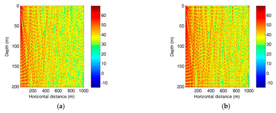
Figure 10.
Two-dimensional color figure of SPL using combined WSM and FEM (100 Hz). (a) Combined WSM; (b) FEM.
The field interference fringes in Figure 10a are clear, and the results are similar to the finite element results in Figure 10b. Same as in Figure 10b, Figure 10a can also describe the phenomenon caused by the interaction of radiated sound with the sea surface and the sea bottom during the propagation of the sound, that is, the sound rays reflect back and forth between the sea surface and the sea bottom. However, the difference is that compared with Figure 10b, the peak and trough amplitudes of Figure 10a are not clear enough, which is also reflected in Figure 7.
It should be noted that in order for combined WSM to accurately predict the radiated field of the structure, the environment of the sea needs to meet the applicable range of ray theory. The following relationships can be used as a guide for high-frequency approximation of ray theory [1] as shown as:
where is the frequency, is sound speed in water, and is the depth of the water. This relationship can also be used as guidance for the applicable conditions of combined WSM. Although the guidance given by this relationship is not necessarily accurate, it can indeed reflect the potential of combined WSM for the calculation of high-frequency problems.
4. Conclusions
In this paper, a new method is proposed for the prediction of radiated acoustic field in shallow sea. Ray theory is a high frequency approximation theory with high accuracy and high computational efficiency. On the basis of the wave superposition method, the application range of the wave superposition method is expanded by introducing the ray theory. Since the Green’s function in sea is a cylindrical function, a high-order superposition is required to ensure accuracy, while the distance between the virtual source surface and the surface of the structure cannot be too close. In addition, the structural surface vibration velocity nodes and the virtual sources should avoid overlapping in the vertical direction as much as possible, which should be paid attention to, while constructing the virtual source surface. After comparison with examples, it is verified that the proposed method is accurate. It can be used to analyze the acoustic radiation of complex structures under water and have potential for the calculation of high-frequency problems.
Author Contributions
Conceptualization, D.S.; methodology, C.Z. and Y.L.; software, Y.L.; validation, C.Z., Y.L. and D.S.; formal analysis, Y.L.; investigation, Y.L.; resources, D.S.; data curation, D.S.; writing—original draft preparation, C.Z. and Y.L.; writing—review and editing, I.U.K.; visualization, Y.L.; supervision, D.S.; project administration, D.S.; funding acquisition, C.Z. and D.S. All authors have read and agreed to the published version of the manuscript.
Funding
This work was supported by “the Fundamental Research Funds for the Central Universities, HEU” (Grant No. 3072019CF0505) and the Stable Supporting Fund of Acoustic Science and Technology Laboratory (Grant No. JCKYS2019604SSJS009).
Conflicts of Interest
The authors declare no conflict of interest.
References
- Etter, P.C. Underwater Acoustic Modeling and Simulation; CRC Press: Boca Raton, FL, USA, 2018. [Google Scholar]
- Pierce, A.D. Extension of the method of normal modes to sound propagation in an almost-stratified medium. J. Acoust. Soc. Am. 1965, 37, 19–27. [Google Scholar] [CrossRef]
- Evans, R.B. A coupled mode solution for acoustic propagation in a waveguide with stepwise depth variations of a penetrable bottom. J. Acoust. Soc. Am. 1983, 74, 188–195. [Google Scholar] [CrossRef]
- Schmidt, H.; Glattetre, J. A fast field model for three-dimensional wave propagation in stratified environments based on the global matrix method. J. Acoust. Soc. Am. 1985, 78, 2105–2114. [Google Scholar] [CrossRef]
- Collis, J.M.; Siegmann, W.L.; Jensen, F.B.; Zampolli, M.; Küsel, E.T.; Collins, M.D. Parabolic equation solution of seismo-acoustics problems involving variations in bathymetry and sediment thickness. J. Acoust. Soc. Am. 2008, 123, 51–55. [Google Scholar] [CrossRef] [PubMed]
- Koopmann, G.H.; Song, L.; Fahnline, J.B. A method for computing acoustic felds based on the principle of wave superposition. J. Acoust. Soc. Am. 1989, 86, 2433–2438. [Google Scholar] [CrossRef]
- Song, L.; Koopmann, G.H.; Fahnline, J.B. Numerical errors associated with the method of superposition for computing acoustic felds. J. Acoust. Soc. Am. 1991, 89, 2625–2633. [Google Scholar] [CrossRef]
- Miller, R.D.; Moyer, E.T., Jr.; Huang, H.; Überall, H. A comparison between the boundary element method and the wave superposition approach for the analysis of the scattered felds from rigid bodies and elastic shells. J. Acoust. Soc. Am. 1991, 89, 2185–2196. [Google Scholar] [CrossRef]
- Fahnline, J.B.; Koopmann, G.H. A numerical solution for the general radiation problem based on the combined methods of superposition and singular-value decomposition. J. Acoust. Soc. Am. 1991, 90, 2808–2819. [Google Scholar] [CrossRef]
- Bi, C.-X.; Jing, W.-Q.; Zhang, Y.-B.; Lin, W.-L. Reconstruction of the sound feld above a reflecting plane using the equivalent source method. J. Sound Vib. 2017, 386, 149–162. [Google Scholar] [CrossRef]
- Jeans, R.; Mathews, I. The wave superposition method as a robust technique for computing acoustic felds. J. Acoust. Soc. Am. 1992, 92, 1156–1166. [Google Scholar] [CrossRef]
- De-Jiang, S.; Zhi-Wen, Q.; Yuan-An, H.; Yan, X. Sound radiation of cylinder in shallow water investigated by combined wave superposition method. Acta Phys. Sin. 2018, 67, 125–138. [Google Scholar]
- Qian, Z.; Shang, D.; He, Y. Sound radiation from a cylinder in shallow water by fem and pe method. J. Acoust. Soc. Am. 2018, 143, 1927. [Google Scholar] [CrossRef]
- Jensen, F.B.; Kuperman, W.A.; Porter, M.B.; Schmidt, H. Computational Ocean Acoustics; Springer Science & Business Media: Berlin/Heidelberg, Germany, 2011. [Google Scholar]
- Golub, G.H.; Hansen, P.C.; O’Leary, D.P. Tikhonov regularization and total least squares. SIAM J. Matrix Anal. Appl. 1999, 21, 185–194. [Google Scholar] [CrossRef]
- Liu, B.S.; Lei, J.Y. Underwater Acoustics Principle; Harbin Shipbuilding Engineering Institute Press: Harbin, China, 1993. [Google Scholar]
- Apel, J.R. Principles of Ocean Physics; Academic Press: Cambridge, MA, USA, 1987; Volume 38. [Google Scholar]
- Westwood, E.K.; Vidmar, P.J. Eigenray fnding and time series simulation in a layeredbottom ocean. J. Acoust. Soc. Am. 1987, 81, 912–924. [Google Scholar] [CrossRef]
- Li, J.-Q.; Chen, J.Y.; Chao, J.W.-Q. Analysis of the impact factors on the accuracy of sound feld reconstruction based on wave superposition. Acta Phys. Sin. 2008, 7, 4258–4264. [Google Scholar]
© 2020 by the authors. Licensee MDPI, Basel, Switzerland. This article is an open access article distributed under the terms and conditions of the Creative Commons Attribution (CC BY) license (http://creativecommons.org/licenses/by/4.0/).