Musical Emotion Recognition with Spectral Feature Extraction Based on a Sinusoidal Model with Model-Based and Deep-Learning Approaches

Abstract
1. Introduction
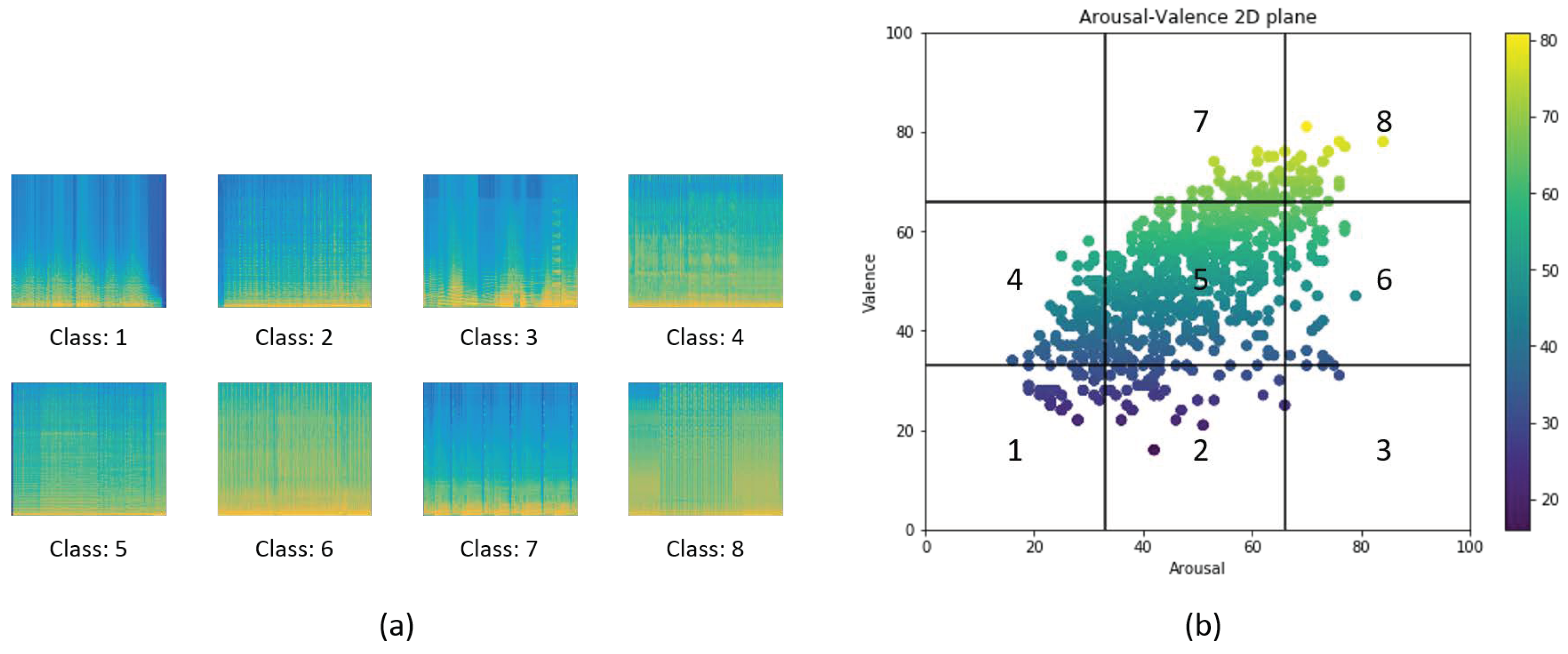
2. Database
3. Proposed Method
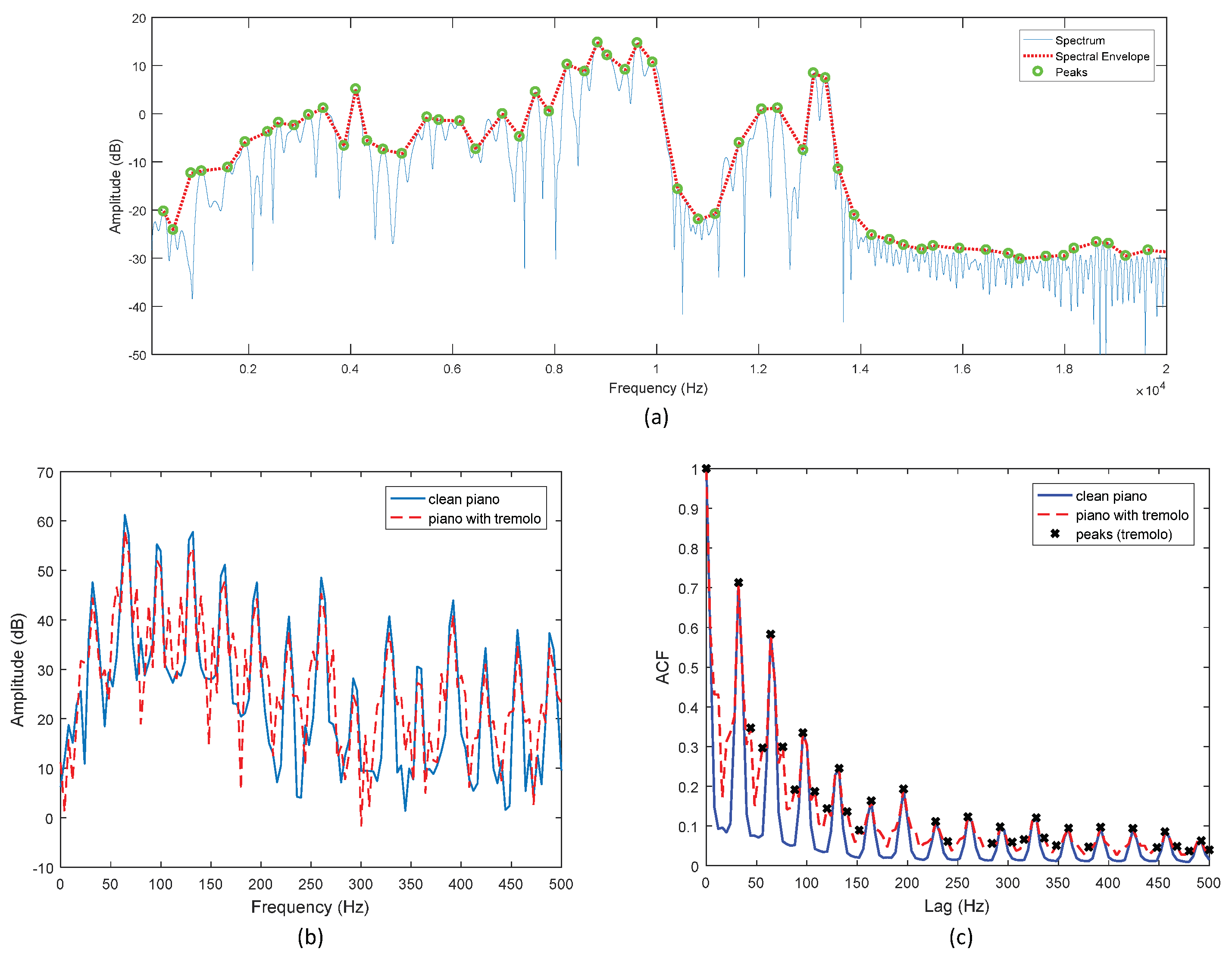
3.1. Sinusoidal Transform Coding
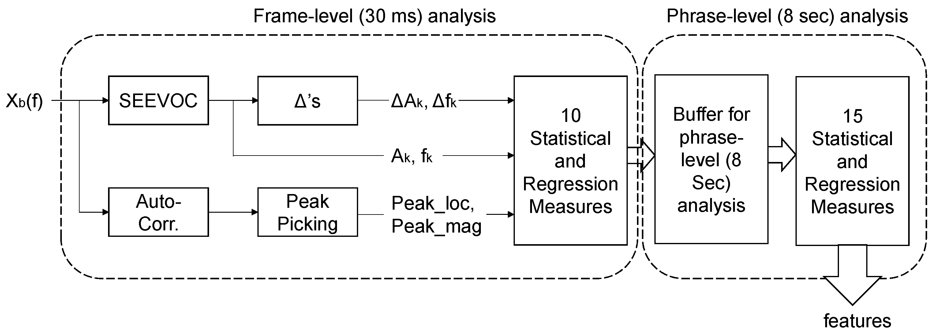
3.2. Feature Extraction Using Sinusoidal Transform Coding
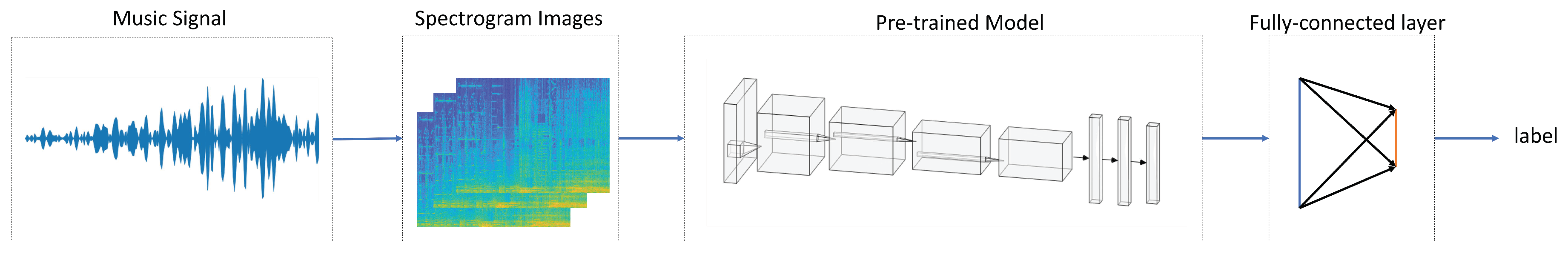
3.3. Feature Extraction Using Transfer Learning
4. Experimental Results
4.1. Model-Based Approach Based on Spectral Features and Conventional Machine Learning Algorithms
4.2. Deep Learning Approach Using Transfer Learning
5. Conclusions
Author Contributions
Funding
Conflicts of Interest
References
- Baltrunas, L.; Amatriain, X. Towards time-dependant recommendation based on implicit feedback. In Proceedings of the Workshop on Context-Aware Recommender Systems (CARS’09), New York, NY, USA, 25 October 2009. [Google Scholar]
- Kim, J.C.; Azzi, P.; Jeon, M.; Howard, A.M.; Park, C.H. Audio-based emotion estimation for interactive robotic therapy for children with autism spectrum disorder. In Proceedings of the 2017 14th International Conference on Ubiquitous Robots and Ambient Intelligence (URAI), Jeju, Korea, 28 June–1 July 2017; pp. 39–44. [Google Scholar]
- Aucouturier, J.J.; Pachet, F.; Sandler, M. “The way it sounds”: Timbre models for analysis and retrieval of music signals. IEEE Trans. Multimed. 2005, 7, 1028–1035. [Google Scholar] [CrossRef]
- Kim, J.; Clements, M. Time-scale modification of audio signals using multi-relative onset time estimations in sinusoidal transform coding. In Proceedings of the 2010 Conference Record of the Forty Fourth Asilomar Conference on Signals, Systems and Computers, Pacific Grove, CA, USA, 7–10 November 2010; pp. 558–561. [Google Scholar]
- Serra, X.; Smith, J. Spectral modeling synthesis: A sound analysis/synthesis system based on a deterministic plus stochastic decomposition. Comput. Music J. 1990, 14, 12–24. [Google Scholar] [CrossRef]
- Quatieri, T.F.; McAulay, R.J. Shape invariant time-scale and pitch modification of speech. IEEE Trans. Signal Process. 1992, 40, 497–510. [Google Scholar] [CrossRef]
- Kim, J.C.; Rao, H.; Clements, M.A. Speech intelligibility estimation using multi-resolution spectral features for speakers undergoing cancer treatment. J. Acoust. Soc. Am. 2014, 136, EL315–EL321. [Google Scholar] [CrossRef] [PubMed]
- Satt, A.; Rozenberg, S.; Hoory, R. Efficient Emotion Recognition from Speech Using Deep Learning on Spectrograms. In Proceedings of the INTERSPEECH 2017, Stockholm, Sweden, 20–24 August 2017; pp. 1089–1093. [Google Scholar]
- Badshah, A.M.; Ahmad, J.; Rahim, N.; Baik, S.W. Speech emotion recognition from spectrograms with deep convolutional neural network. In Proceedings of the 2017 International Conference on Platform Technology and Service (PlatCon), Busan, Korea, 13–15 Feburary 2017; pp. 1–5. [Google Scholar]
- Soleymani, M.; Caro, M.N.; Schmidt, E.M.; Sha, C.Y.; Yang, Y.H. 1000 songs for emotional analysis of music. In Proceedings of the 2nd ACM International Workshop on Crowdsourcing for Multimedia, Barcelona, Spain, 22 October 2013; ACM: New York, NY, USA, 2013; pp. 1–6. [Google Scholar]
- Aljanaki, A.; Yang, Y.H.; Soleymani, M. Emotion in Music Task at MediaEval 2014; MediaEval: Barcelona, Spain, 2014. [Google Scholar]
- Eyben, F.; Wöllmer, M.; Schuller, B. Opensmile: The munich versatile and fast open-source audio feature extractor. In Proceedings of the 18th ACM International Conference on Multimedia, Firenze, Italy, 25–29 October 2010; ACM: New York, NY, USA, 2010; pp. 1459–1462. [Google Scholar]
- Pantazis, Y.; Rosec, O.; Stylianou, Y. Adaptive AM–FM signal decomposition with application to speech analysis. IEEE Trans. Audio Speech Lang. Process. 2010, 19, 290–300. [Google Scholar] [CrossRef]
- George, E.B.; Smith, M.J. Analysis-by-synthesis/overlap-add sinusoidal modeling applied to the analysis and synthesis of musical tones. J. Audio Eng. Soc. 1992, 40, 497–516. [Google Scholar]
- Paul, D. The spectral envelope estimation vocoder. IEEE Trans. Acoust. Speech Signal Process. 1981, 29, 786–794. [Google Scholar] [CrossRef]
- Jusczyk, P.W.; Krumhansl, C.L. Pitch and rhythmic patterns affecting infants’ sensitivity to musical phrase structure. J. Exp. Psychol. Hum. Percept. Perform. 1993, 19, 627. [Google Scholar] [CrossRef] [PubMed]
- Jensen, J.H.; Christensen, M.G.; Ellis, D.P.; Jensen, S.H. A tempo-insensitive distance measure for cover song identification based on chroma features. In Proceedings of the 2008 IEEE International Conference on Acoustics, Speech and Signal Processing, Las Vegas, NV, USA, 31 March–4 April 2008; pp. 2209–2212. [Google Scholar]
- Pan, S.J.; Yang, Q. A survey on transfer learning. IEEE Trans. Knowl. Data Eng. 2009, 22, 1345–1359. [Google Scholar] [CrossRef]
- Kim, J.C.; Clements, M.A. Multimodal affect classification at various temporal lengths. IEEE Trans. Affect. Comput. 2015, 6, 371–384. [Google Scholar] [CrossRef]
- Metallinou, A.; Wollmer, M.; Katsamanis, A.; Eyben, F.; Schuller, B.; Narayanan, S. Context-sensitive learning for enhanced audiovisual emotion classification. IEEE Trans. Affect. Comput. 2012, 3, 184–198. [Google Scholar] [CrossRef]
- Russell, J.A.; Bachorowski, J.A.; Fernández-Dols, J.M. Facial and vocal expressions of emotion. Annu. Rev. Psychol. 2003, 54, 329–349. [Google Scholar] [CrossRef] [PubMed]
- Hailstone, J.C.; Omar, R.; Henley, S.M.; Frost, C.; Kenward, M.G.; Warren, J.D. It’s not what you play, it’s how you play it: Timbre affects perception of emotion in music. Q. J. Exp. Psychol. 2009, 62, 2141–2155. [Google Scholar] [CrossRef] [PubMed]
- Simonyan, K.; Zisserman, A. Very deep convolutional networks for large-scale image recognition. arXiv 2014, arXiv:1409.1556. [Google Scholar]
- Krizhevsky, A. One weird trick for parallelizing convolutional neural networks. arXiv 2014, arXiv:1404.5997. [Google Scholar]
- Szegedy, C.; Vanhoucke, V.; Ioffe, S.; Shlens, J.; Wojna, Z. Rethinking the inception architecture for computer vision. In Proceedings of the IEEE Conference on Computer Vision and Pattern Recognition, Las Vegas, NV, USA, 27–30 June 2016; pp. 2818–2826. [Google Scholar]
- He, K.; Zhang, X.; Ren, S.; Sun, J. Deep residual learning for image recognition. In Proceedings of the IEEE Conference on Computer Vision and Pattern Recognition, Las Vegas, NV, USA, 27–30 June 2016; pp. 770–778. [Google Scholar]
- Huang, G.; Liu, Z.; Van Der Maaten, L.; Weinberger, K.Q. Densely connected convolutional networks. In Proceedings of the IEEE Conference on Computer Vision and Pattern Recognition, Honolulu, HI, USA, 21–26 July 2017; pp. 4700–4708. [Google Scholar]
- Xie, S.; Girshick, R.; Dollár, P.; Tu, Z.; He, K. Aggregated residual transformations for deep neural networks. In Proceedings of the IEEE Conference on Computer Vision and Pattern Recognition, Honolulu, HI, USA, 21–26 July 2017; pp. 1492–1500. [Google Scholar]


| Num. | Description |
|---|---|
| 1 | maximum |
| 2 | minimum |
| 3 | mean * |
| 4 | standard deviation |
| 5 | kurtosis * |
| 6 | skewness |
| 7∼9 | 1 st, 2 nd, & 3 rd quartiles * |
| 10 | interquartile range * |
| 11∼12 | 1 st & 99 th percentiles * |
| 13 | RMS value |
| 14 | slope of linear regression * |
| 15 | approximation error of linear regression * |
| RMSE | ||||||
| Arousal | Valence | |||||
| PLS | PCR | FF | PLS | PCR | FF | |
| base. | 0.146 | 0.147 | 0.172 | 0.156 | 0.156 | 0.169 |
| STC | 0.149 | 0.150 | 0.179 | 0.156 | 0.157 | 0.172 |
| base+STC | 0.144 | 0.144 | 0.165 | 0.151 | 0.150 | 0.158 |
| Peason’s coefficient | ||||||
| Arousal | Valence | |||||
| PLS | PCR | FF | PLS | PCR | FF | |
| base. | 0.785 | 0.781 | 0.732 | 0.601 | 0.612 | 0.570 |
| STC | 0.775 | 0.770 | 0.730 | 0.600 | 0.585 | 0.551 |
| base+STC | 0.793 | 0.793 | 0.754 | 0.630 | 0.634 | 0.609 |
| Performance Comparison | ||||
|---|---|---|---|---|
| Model Name | Top-1 Acc. | Top-5 Acc. | Best Performance | Trainable Params. |
| VGG-11 | 64.79 ± 1.51% | 95.52 ± 2.17% | 66.56% | 32,776 |
| VGG-13 | 65.05 ± 1.32% | 96.62 ± 1.83% | 65.61% | 32,776 |
| VGG-16 | 64.77 ± 1.44% | 96.36 ± 2.08% | 66.93% | 32,776 |
| VGG-19 | 64.58 ± 1.49% | 95.86 ± 2.06% | 66.77% | 32,776 |
| AlexNet | 65.00 ± 1.01% | 96.07 ± 1.74% | 65.61% | 32,776 |
| Inception-V3 | 64.53 ± 1.44% | 95.36 ± 1.64% | 66.40% | 16,392 |
| ResNet-18 | 64.86 ± 1.16% | 95.45 ± 2.05% | 66.78% | 4104 |
| ResNet-34 | 65.04 ± 1.34% | 95.85 ± 1.91% | 66.72% | 4104 |
| ResNet-50 | 65.24 ± 1.35% | 95.63 ± 1.66% | 67.42% | 16,392 |
| ResNet-101 | 65.11 ± 1.35% | 96.23 ± 1.84% | 67.10% | 16,392 |
| ResNet-152 | 65.31 ± 1.02% | 95.92 ± 1.69% | 66.61% | 16,392 |
| DenseNet-121 | 64.79 ± 1.37% | 95.64 ± 2.36% | 67.26% | 8200 |
| DenseNet-169 | 64.94 ± 1.45% | 96.68 ± 2.13% | 67.10% | 13,320 |
| DenseNet-201 | 64.67 ± 1.32% | 96.91 ± 2.05% | 66.45% | 15,368 |
| ResNext-50 | 65.45 ± 1.29% | 96.17 ± 2.38% | 67.10% | 16,392 |
| ResNext-101 | 65.31 ± 1.02% | 96.26 ± 1.91% | 66.61% | 16,392 |
© 2020 by the authors. Licensee MDPI, Basel, Switzerland. This article is an open access article distributed under the terms and conditions of the Creative Commons Attribution (CC BY) license (http://creativecommons.org/licenses/by/4.0/).
Share and Cite
Xie, B.; Kim, J.C.; Park, C.H. Musical Emotion Recognition with Spectral Feature Extraction Based on a Sinusoidal Model with Model-Based and Deep-Learning Approaches. Appl. Sci. 2020, 10, 902. https://doi.org/10.3390/app10030902
Xie B, Kim JC, Park CH. Musical Emotion Recognition with Spectral Feature Extraction Based on a Sinusoidal Model with Model-Based and Deep-Learning Approaches. Applied Sciences. 2020; 10(3):902. https://doi.org/10.3390/app10030902
Chicago/Turabian StyleXie, Baijun, Jonathan C. Kim, and Chung Hyuk Park. 2020. "Musical Emotion Recognition with Spectral Feature Extraction Based on a Sinusoidal Model with Model-Based and Deep-Learning Approaches" Applied Sciences 10, no. 3: 902. https://doi.org/10.3390/app10030902
APA StyleXie, B., Kim, J. C., & Park, C. H. (2020). Musical Emotion Recognition with Spectral Feature Extraction Based on a Sinusoidal Model with Model-Based and Deep-Learning Approaches. Applied Sciences, 10(3), 902. https://doi.org/10.3390/app10030902