Considering Uncertainties of Key Performance Indicators in Wind Turbine Operation

Featured Application

The results enable wind turbine operational managers to consider data handling-related uncertainties when using KPIs. The following recommendations allow mitigating uncertainties through simple measures. Furthermore, methods are proposed to correct systematic deviations.

Abstract

Key performance indicators (KPIs) are commonly used in the wind industry to support decision-making and to prioritize the work throughout a wind turbine portfolio. Still, there is little knowledge of the uncertainties of KPIs. This article intends to shed some light on the uncertainty and reliability of KPIs in general and performance KPIs in particular. For this purpose, different uncertainty causes are discussed, and three data handling related uncertainty causes are analyzed in detail for five KPIs. A local sensitivity analysis is followed by a more detailed analysis of the related uncertainties. The work bases on different sets of operational data, which are manipulated in a large number of experiments to carry out an empirical uncertainty analysis. The results show that changes in the data resolution, data availability, as well as missing inputs, can cause considerable uncertainties. These uncertainties can be reduced or even mitigated by simple measures in many cases. This article provides a comprehensive list of statements and recommendations to estimate the relevance of data handling related KPI uncertainties in the day-to-day work as well as approaches to correct KPIs for systematic deviations and simple steps to avoid pitfalls.

1. Introduction

After the successful installation of a wind farm (WF), the operational performance of its wind turbines (WTs) determines whether a project is economically successful or not. On average, operation and maintenance (O&M) accounts for approximately 25% to 35% [1,2,3,4] of the levelized cost of energy (LCOE) and also affects the energetic and monetary revenue. Thus, the performance of WTs is of high importance and closely monitored by operational managers. As part of the digitalization of energy supply, the latest information technology (IT) applications and solutions also penetrate the area of O&M of WTs and WFs. Big data and artificial intelligence (AI) applications in particular support the operational managers with valuable information regarding the WT performance. As more and more tasks and evaluations are automated, reliable and trustworthy results become more important.

KPIs are a common tool throughout all industries to make information easily accessible and comparable [5]. The wind industry is no exception and makes use of KPIs to evaluate the performance and reliability of WTs regularly. A whole set of KPIs is used to evaluate different aspects of WT operation, as shown in [6,7]. Even though further tools like sophisticated machine learning approaches for condition monitoring systems (cms) [8] and performance monitoring applications [9] are used more and more often in the industry; KPIs remain the foundation for asset management, reporting, and benchmarking. As KPIs and their trends are part of many decision-making processes, it is necessary to take their reliability into account [5].

The reliability of a KPI can also be referred to as its uncertainty. Even though the uncertainties of KPIs have not been widely discussed in the literature, a few publications are available. Sánchez-Márquez et al. [10] evaluate the uncertainties of KPIs used for balanced scorecards caused by the selected sample size. Perotto et al. [11] discuss the uncertainty of environmental performance indicators on wastewater discharges, and Torregrossa et al. [12] deal with the uncertainty of energy consumption indicators for wastewater treatment plants due to measurement uncertainties and data availability limitations. Another example is the consideration of uncertainties by Feiz et al. [13] for a CO₂ emission indicator used in the cement industry.

Publications on the sensitivity and uncertainty of KPIs related to the wind industry are rare. Martin et al. [14] perform an analysis of the sensitivity of O&M costs on the chosen maintenance strategy; although this approach aims to identify cost reduction factors and not to identify and quantify uncertainties. The work of Dykes et al. [15] follows a similar approach and performs a sensitivity analysis of the wind plant performance to changes in WT design parameters. The only known publication on uncertainties of a performance KPI for WT operation was published by Craig et al. [16], which examines the uncertainty in power curves due to different methods for data filtering and power curve modeling. This work is continued in another publication [17] to quantify the uncertainties of wind plant energy estimation resulting from power curve uncertainties and different sampling periods.

A broader assessment of the uncertainties of O&M-KPIs used in the monitoring of WT is lacking. Thus, this paper discusses sensitivities and uncertainties of the most important performance KPIs and tries to quantify uncertainties to assess their relevance for the daily work. Another scope of this paper is to provide recommendations to reduce or mitigate KPI uncertainties by simple measures. The results are also meant to raise awareness of uncertainties when dealing with KPIs in general. The authors try to view uncertainties from the perspective of an operational manager and consider uncertainties that are relevant to and can be influenced by this specific role. By quantifying KPI uncertainties and providing mitigation strategies, this paper aims at more reliable and trustworthy KPIs as part of decision support tools.

2. Key Performance Indicators

In operational management of WTs, KPIs are used to evaluate and categorize the performance of WTs with regard to (1.) Predetermined target values, which are in many cases part of contractual agreements, (2.) comparable WTs (e.g., of the same WF), or (3.) the long-term trend of the WT itself. In any case, KPIs are always compared to a reference, and significant deviations usually trigger actions [18,19].

A high deviation to the reference reflects a high need for intervention and leads to a higher prioritization in the work of an operational manager. This usually means a more detailed review of the performance of the WT and the operational data to identify the underlying causes. At this point, one has to ask what deviation to the reference value can be considered to be healthy or can be explained due to the uncertainty of the KPI itself, and thus either should not trigger any action or lower its priority. To answer this question is one of the main scopes of the present work.

As a single KPI is usually not sufficient to rate the performance of a WT, in most cases, a set of different metrics is used. The selected KPIs are calculated on a regular base. Monthly, quarterly, half-yearly, and yearly periods are common resolutions for KPIs and are normally synchronized with reporting periods [18,19]. According to Gonzalez et al. [7] and Pfaffel et al. [6], KPIs for O&M of WTs belong to one of the following five different groups.

• Performance KPIs
• Maintenance KPIs
• Reliability KPIs
• Health, Safety and the Environment (HSE) KPIs
• Finance KPIs

Financial and HSE KPIs are not wind-specific, and are thus excluded from further evaluation. Furthermore, the calculation of HSE, reliability, and some maintenance KPIs is solely based on distinct events instead of measurements. As the idea to provide uncertainties for theses KPIs is misleading, they are excluded as well. According to Hahn et al. [20], standardization of the collected data and a review of documentation processes provides much more utility in this case. To select a total of five KPIs for further assessment out of the remaining KPIs, the prioritization of KPIs, as provided by [6], is used. The selected KPIs are briefly described and defined in Section 2.1, Section 2.2, Section 2.3 and Section 2.4 based on [6].

2.1. Wind Conditions

The wind conditions define the quality of a specific WT site and are not a KPI itself but described by several KPIs. The most known KPI is the average wind speed, see Equation (1). As it reflects the usable energy inadequately, the authors complemented it by the average wind power density for this publication, see Equation (2). The wind power density includes the cubic relation between wind speed and the usable energy, and also considers varying air densities. Both KPIs are calculated based on n observations in the observation period (e.g., day, month, year).

$$\overline{V}=\frac{1}{n}·{\displaystyle \sum _{i=1}^n}{V}_{\mathrm{i}}$$

(1)

where

$$\begin{array}{cc}\overline{V}\hfill & =\mathrm{Average}\mathrm{wind}\mathrm{speed},\hfill \\ V_{\mathrm{i}}\hfill & =\mathrm{Measured}\mathrm{wind}\mathrm{speed}\mathrm{for}\mathrm{the}\mathrm{ith}\mathrm{observation}\hfill \end{array}$$

$${\overline{P}}_{\mathrm{Wind}}=\frac{1}{n}·{\displaystyle \sum _{i=1}^n}\frac{1}{2}{\rho }_{\mathrm{i}}{V}_{\mathrm{i}}^3$$

(2)

where

$$\begin{array}{cc}\hfill {\overline{P}}_{\mathrm{Wind}}& =\mathrm{Average}\mathrm{wind}\mathrm{power}\mathrm{density},\hfill \\ \hfill {\rho }_{\mathrm{i}}& =\mathrm{Air}\mathrm{density}\mathrm{for}\mathrm{the}\mathrm{ith}\mathrm{observation},\hfill \\ \hfill V_{\mathrm{i}}& =\mathrm{Measured}\mathrm{wind}\mathrm{speed}\mathrm{for}\mathrm{the}\mathrm{ith}\mathrm{observation}\hfill \end{array}$$

2.2. Capacity Factor

The capacity factor normalizes the energy yield to the rated power of a WT, see Equation (3). It is a common metric to compare WTs of the same WF or review the long term trend of a specific WT.

$$CF=\frac{W_{\mathrm{Actual}}}{W_{\mathrm{Nominal}}}·100\%$$

(3)

where

$$\begin{array}{cc}\hfill CF& =\mathrm{Capacity}\mathrm{factor}\hfill \\ \hfill W_{\mathrm{Actual}}& =\mathrm{Actual}\mathrm{energy}\mathrm{yield}\mathrm{of}\mathrm{the}\mathrm{observation}\mathrm{period},\hfill \\ \hfill W_{\mathrm{Nominal}}& =\mathrm{Nominal}\mathrm{possible}\mathrm{energy}\mathrm{yield}\mathrm{of}\mathrm{the}\mathrm{observation}\mathrm{period}\hfill \end{array}$$

2.3. Power Curve

The power curve is not a KPI itself but an essential tool in WT monitoring, and is also necessary to calculate further KPIs. It represents the relation between wind speed and power output of a WT. Exemplary use cases for power curves during the operational period of a WT are a basic monitoring of the WT performance through a visualization of the operating data or the calculation of energy losses during downtimes.

2.4. Production-Based Availability

The production-based availability is the ratio between the actual energy yield and the potential energy yield of a WT if downtimes would not occur (actual yield plus energy losses), see Equation (4). Compared to the time-based availability, downtimes are weighted by their energy losses. The corresponding energy losses can be determined using several methods, inter alia by using the power curve and wind speed measurements.

$$A_W=\left(1-\frac{W_{\mathrm{Potential}}-W_{\mathrm{Actual}}}{W_{\mathrm{Potential}}}\right)·100\%$$

(4)

where

$$\begin{array}{cc}\hfill A_W& =\mathrm{Production}-\mathrm{based}\mathrm{availability},\hfill \\ \hfill W_{\mathrm{Actual}}& =\mathrm{Actual}\mathrm{energy}\mathrm{yield}\mathrm{of}\mathrm{the}\mathrm{observation}\mathrm{period},\hfill \\ \hfill W_{\mathrm{Potential}}& =\mathrm{Potential}\mathrm{energy}\mathrm{yield}\mathrm{of}\mathrm{the}\mathrm{observation}\mathrm{period}\hfill \end{array}$$

3. Uncertainties

“Uncertainty” is a term and concept used in various ways. Lindley [21] describes it generically to be a situation where one does not know whether a statement or information is true or false. According to the Guide to the Expression of Uncertainty in Measurement (GUM) [22], it “means doubt about the validity of the result of a measurement”. This definition, in the context of measurements and metrics that also includes KPIs, corresponds to the idea of this work.

Uncertainties are closely related to sensitivities. Sensitivity analyses evaluate the effect of single parameters or a group of parameters on a result and are, for example, also used when assessing different scenarios. In the context of uncertainties, a sensitivity analysis helps to understand whether and how substantial deviations of one parameter affect the measurement or KPI and is performed as the first step of an uncertainty analysis. Sensitivity analyses can be distinguished into local and global analyses. A local sensitivity analysis evaluates the impact of deviations of an isolated parameter while keeping the other inputs stable, whereas a global sensitivity analysis varies all input parameters at the same time so that interdependencies can be discovered. Screening methods combine both attempts [22,23].

Uncertainties are either aleatoric or epistemic. Aleatoric uncertainties are caused by the natural randomness of processes and are thus not predictable. Epistemic uncertainties are the result of a lack of information or knowledge and can be avoided or corrected in theory. [24] The standard deviation ($\sigma$) is a common metric to quantify uncertainties and assumes that the related results follow a normal distribution [22]. Density functions of single uncertainties can be combined to overall uncertainties through analytical or numerical methods. For this purpose, it is vital to know whether single uncertainties are independent or not [25,26,27,28].

Utilization of uncertainties in the wind industry includes the determination of wind potential and energy yields [29], the determination of power curves [30,31], or wind power forecasts [32,33]. The results in corresponding expert reports, measurements, or predictions are displayed with uncertainty information to enable the consideration of individual safety requirements in decision-making processes. The only known publication related to uncertainties of KPIs in the wind industry is the already mentioned work of Craig et al. [16] on the uncertainty of power curves.

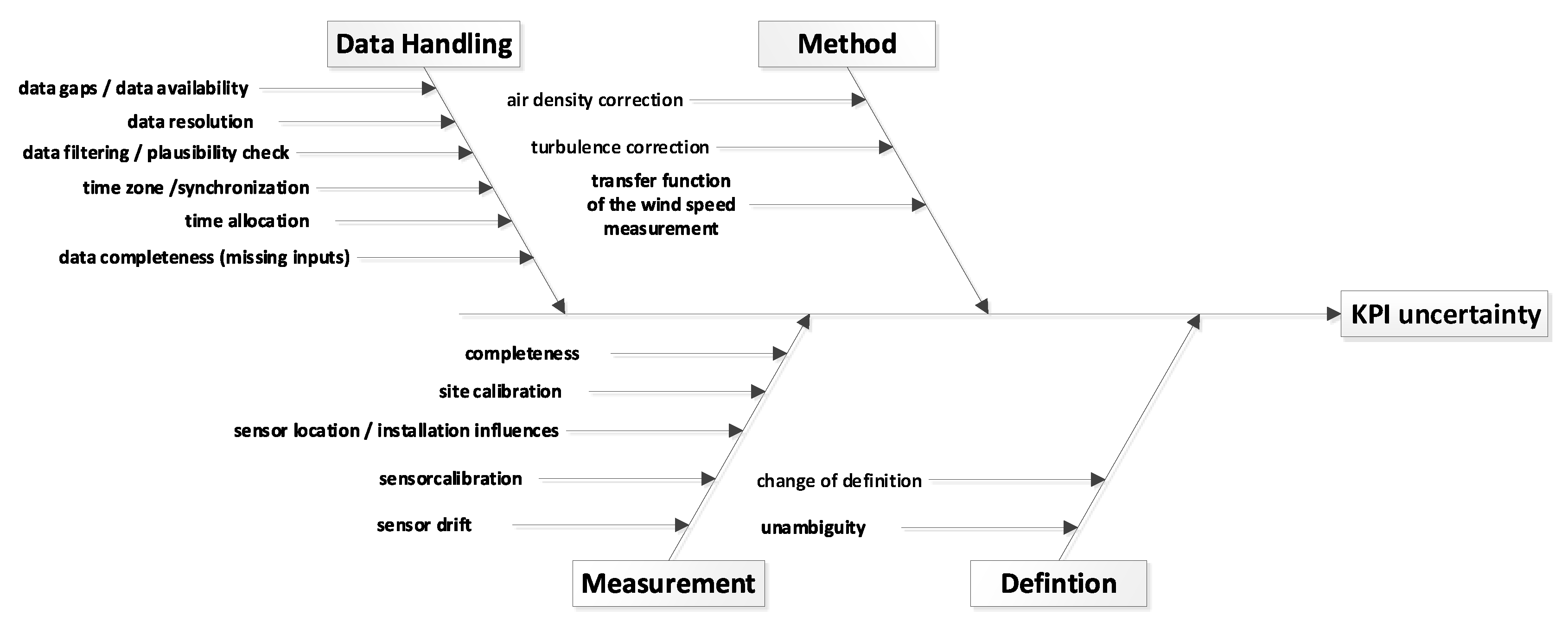
Figure 1 presents a fishbone diagram of possible causes of uncertainties collected for this work. The single causes haven been assigned to one of the four groups: data handling, measurement, method, and definition. As data handling-related uncertainties are the only uncertainties that are, to a certain extent, in control of the operational manager, this work focuses on this group. The other groups are briefly discussed below.

Measurement uncertainties are the apparent causes of uncertainties for KPIs and well researched in general. Relevant references for uncertainties of inputs like power, wind speed, wind direction, and temperature are the International Electrotechnical Commission (IEC) standards 61400-12-1/2 [30,31] (tables G1–G8) and 61400-15 [34], the technical guideline six [29] of the Fördergesellschaft Windenergie und andere Dezentrale Energien (FGW e.V.), and the recommendations of the Measuring Network of Wind Energy Institutes (MEASNET) [35]. Default or standard values for individual uncertainties of the measurements are also given in the sources mentioned.

Uncertainties resulting from corrections to the measured values are assigned to the uncertainty group “method”. Among other factors, the wind speed measurement of the nacelle anemometer is corrected by a transfer function to account for the slowed down and disturbed wind speed at the measuring position behind the rotor. When determining a power curve, the wind speed is also corrected to reference values for turbulence and air density, for example. Further details on the methods and the associated uncertainties can be found in the IEC standard 61400-12-1/2 [30,31].

Further uncertainties can arise when KPI definitions are changed, different definitions are used or from an inaccurate formulation of the definition. As KPIs are usually calculated and compared in a closed operational management software or benchmark platform, consistent definitions can be assumed for the entire portfolio and all periods. However, this uncertainty group should be considered whenever precalculated KPIs from different sources or systems are compared. The IEC standard 61400-26-1/2 [36,37] already provides four exemplary definitions of the time-based availability and three definitions of the production-based availability, let alone many more company-specific versions.

Data handling related uncertainties originate from the way how data are collected, processed, and stored. Some of the listed uncertainty causes can be easily avoided by simple measures or proper documentation of the data, and are thus not further investigated. Examples are missing information on the time zone of timestamps, a missing synchronization, or missing information on the time allocation (start, center, end) of an aggregation period. Uncertainties due to different data filtering approaches have been investigated by Craig et al. [16] for power curves. This work focuses on the remaining three uncertainty causes.

• Data resolution: Operational data of WT are mostly stored in resolutions of 5, 10, or 15 min. Older projects also use resolutions as low as 30 min, whereas recent projects sometimes store Hz data. When data is aggregated, information like extreme values gets lost in the averaging process. This behavior is not to be confused with the Nyquist–Shannon sampling theorem, which determines the necessary sampling rate in a measurement [38,39]. The IEC 61400-12 [30,31] requires for example, a minimum sampling rate of 1 Hz for most measurements—ambient temperature or air pressure can also be sampled once per minute—whereas it defines aggregated 10 min data to be the foundation for power curve calculations. This work expects the underlying measurement to be done correctly. An additional uncertainty cause is related to the sample length of an aggregation period. Whenever samples are missing in the aggregation period, the remaining samples are weighted more strongly than in other periods. Although missing samples might show up in Hz data, they might not be detectable in 5 min data anymore. Schmiedel [40] investigated the information loss when switching from 1 min data to 15 min data in a different context.
• Data gaps/data availability: Data gaps in a long history of operational data are normal. As shown in [41], the data availability is, on average, at 95%. In most cases, the data availability is higher (median at 99%), but in other cases also much lower. Current data availability requirements seem somewhat arbitrary. The German guideline for site assessment [29] requires, for example, a data availability of 80% without any further notices or restrictions. The technical guideline 10 of the FGW e.V. [42] allocates data gaps to be downtime in its availability calculation. Reasons or data gaps are manifold and include failed sensors, downtime of the whole turbine, including its controller, as well as telecommunication interruptions [43]. Many WT still use the GSM standard of the cellular network. If data are missing, the remaining data points are unlikely to be representative of the period considered. Thus, uncertainties in the calculated KPIs are to be expected. Existing literature mainly deals with different approaches to fill data gaps [38,44,45] and not with their effect on KPIs.
• Data completeness: Especially for older WT, the number of available measurements is often very limited, and supporting inputs for the calculation of KPIs are missing. Similar situations occur when sensors fail for a longer time. If the missing measurements are not vital for the calculation but increase the accuracy, they can be neglected or sometimes replaced by approximations. This approach leads in any case to uncertainties. The present paper discusses this issue for the example of air density since it is a vital factor in obtaining comparable results in power performance assessments [30,31]. Especially data sets of older WTs do not comprise all required measurements (air pressure, temperature, and humidity) for an accurate density calculation, which makes our example a common issue in the industry.

4. Method and Data

This work follows the recommendations of the GUM [28] to evaluate different uncertainty causes for various KPIs. In the first step, a local sensitivity analysis determines whether a KPI is affected by a potential uncertainty cause or not. A more detailed analysis is carried out for sensitive relationships to quantify the uncertainties. Herefore, the GUM method “Type A” for the evaluation of standard uncertainties is applied. This approach determines measurement uncertainties through many repeated measurements. The empirical distribution function of all measurements allows calculating the expected value of the measurement as well as the deviations of the single measurements to the expected value. If the distribution function follows a normal distribution, which is commonly assumed for uncertainties, the uncertainty can be quantified by the standard deviation, see Equation (5) [28].

Transferring this method to the present work means calculating KPIs in many experiments either through multiple manipulations of a selected dataset or by investigating many different datasets to determine the expected uncertainty for different scenarios. The described method is intended to quantify the uncertainties due to random (aleatoric) deviations. As the considered uncertainty causes also lead to systematic (epistemic) deviations, as shown later on in the paper, this work also tries to correct or mitigate those systematic deviations.

$$\begin{array}{c}\hfill \sigma =\sqrt{\frac{1}{n}{\displaystyle \sum _{i=1}^n}{(x_i-\mu )}^2}\\ \hfill \mu =\frac{1}{n}{\displaystyle \sum _{i=1}^n}{x}_i{c}_v=\frac{\sigma }{\mu }\end{array}$$

(5)

where

$$\begin{array}{cc}\hfill \sigma & =\mathrm{standard}\mathrm{deviation}\mathrm{over}\mathrm{n}\mathrm{measurements}/\mathrm{experiments},\hfill \\ \hfill x_i& =\mathrm{result}\mathrm{of}\mathrm{the}\mathrm{ith}\mathrm{measurement}/\mathrm{experiment},\hfill \\ \hfill \mu & =\mathrm{average}\mathrm{over}\mathrm{n}\mathrm{measurements}/\mathrm{experiments},\hfill \\ \hfill c_v& =\mathrm{coefficient}\mathrm{of}\mathrm{variation}\hfill \end{array}$$

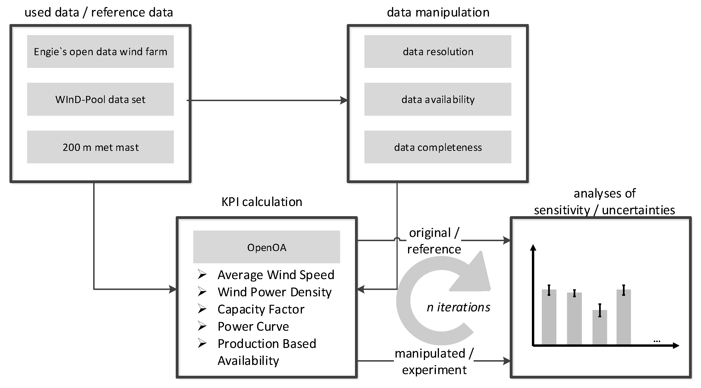
Figure 2 illustrates the overall method of the present paper to determine sensitivities and uncertainties for selected KPIs (Section 2) and uncertainty causes, see Section 4.2, Section 4.3 and Section 4.4 for details. Different data sets (Section 4.1) were used depending on the evaluated uncertainty cause. The approaches for the different uncertainty causes were similar. The original data was used to calculate reference values for the single KPIs. To obtain sufficient data for uncertainty analyses, the original data was manipulated in numerous experiments. In the last step, uncertainties were derived by comparing the results of the experiments to the reference values of the single KPIs.

4.1. Data and Toolset

The present work makes use of several different data sets. To be able to work with a complete and high-quality dataset, comprising all relevant measurements (pressure, temperature, humidity, etc.), the data of a 200 m high wind met mast was analyzed. The met mast is located at a complex, forested site at “Rödeser Berg” close to Kassel in central Germany. The availability of comprehensive meteorological data allows investigating the relevance of complete measurement data for the accuracy of the different KPIs. A detailed description of the location, as well as the instrumentation of the met mast, can be found in a publication by Klaas et al. [46]. Furthermore, data of the Wind Energy Information Data Pool (WInD-Pool) [41] was available where needed. The WInD-Pool includes data in the Hz resolution for a German offshore WF (5 MW WT) in the North Sea, which was needed for this work to evaluate the effect of different resolutions. Further details cannot be stated due to confidentiality reasons. Wherever possible, however, the data from ENGIEs open data WF “La Haute Borne” [47] was used to ensure the replicability of the results. The WF comprises four Senvion MM82 WT with a rated power of 2 MW each and is located in the department Meuse in northeast France. For each WT, operational data over approximately six years was available. All datasets were filtered for implausible values and stuck signals [48], for example, the plausible wind speed range is 0 m/s to 50 m/s.

For the handling, filtering, and manipulation of the data as well as the calculation of KPIs, the Python Open-Source Tool for Wind Farm Operational Performance Analysis (OpenOA) [49,50] was used. OpenOA is developed by the National Renewable Energy Laboratory (NREL) and extended according to the requirements of this work. OpenOA is available under an open source license as Python source code on Github [51]. Due to the public availability of the ENGIE Open-Data-Dataset and OpenOA, the results can be replicated.

4.2. Data Resolution

The effect of different data resolutions was assessed based on 1 Hz data from the WInD-Pool for a 5 MW offshore WT. The dataset comprises of 4,727,951 entries, or 55 days worth, of high-resolution operating data. Data of additional WT was available and used to validate the results. After filtering and merging, 98.5% of the data proved to be good quality, and data gaps were filled by linear interpolation to obtain a continuous and complete time series. This was necessary to investigate the effects of resolution changes without being affected by data gaps and resulting differently weighted data points.

The 1 Hz data was then resampled to different resolutions up to hourly values. Special requirements were also considered, such as for vector functions to average angular values (e.g., wind direction) [30,52]. This averaging process us d the 1 Hz data for each resolution so that sound statistics (min, max, std.) were available. All considered KPIs were then calculated for each resolution to assess sensitivities and uncertainties.

4.3. Data Availability

The relevance of varying data availabilities on different KPIs was assessed based on 10 min data of the WT “R80711” of the ENGIE Open Data WF for the year 2017. Approximately 2% of the data was categorized as implausible values or stuck signals and thus removed. The remaining data serve as the 100% data availability reference for this analysis. In this instance, filling the data gaps was not necessary and would rather falsify the results. In the next step, data gaps were added to the time series to reduce the data availability. This was done in one percent increments for the data availabilities ranging from 100% down to 5%. Two different methods were used to evaluate not only the relevance of the data gaps but also the effect of their distribution in the time series. In the first method, single data gaps were randomly added until the target data availability was reached to achieve a uniform distribution; longer gaps occurred only by chance. The second method added one long subsequent data gap of the required length to reach the targeted data availability by using random starting points.

As every experiment was expected to provide different results, 1000 experiments were carried out per targeted data availability and method to get reliable results. The dataset was split into single months as most KPIs are calculated monthly. Thus, a total of about 2.2 million experiments were carried out. As a single month of data is not sufficient to calculate power curves, they were calculated based on the entire year using the IEC and spline approaches implemented in OpenOA, which totaled in approximately 285,000 power curves.

4.4. Data Completeness

To analyze the effect of missing air density measurements as well as their approximation on the calculation of KPIs, one year of 10 min data of the 200 m met mast was used. This dataset was selected due to its comprehensive, reliable, and well-calibrated measurements. After filtering the data availability of the selected year was 99%. In addition, three years (99.9% data availability) of comprehensive data of a North Sea offshore wf was used, as the met mast does not include power measurements as well as to validate the results.

In the first step, the air density and wind power density sensitivities were evaluated to the availability of temperature, pressure, and humidity measurements using Equation (6) [31], as well as to the site altitude above sea level. Furthermore, the air density was approximated by adding additional inputs step-by-step to assess their relevance starting with the standard atmosphere. All results were compared to a reference case comprised of all required inputs.

$$\rho =\frac{1}{T}\left(\frac{B}{R_0}-\varphi P_w\left(\frac{1}{R_0}-\frac{1}{R_w}\right)\right)$$

(6)

where

$$\begin{array}{cc}\hfill \rho & =\mathrm{derived}\mathrm{air}\mathrm{density},\hfill \\ \hfill T& =\mathrm{measured}\mathrm{absolute}\mathrm{air}\mathrm{temperature},\hfill \\ \hfill B& =\mathrm{measured}\mathrm{air}\mathrm{pressure},\hfill \\ \hfill R_0& =\mathrm{gas}\mathrm{constant}\mathrm{of}\mathrm{dry}\mathrm{air}287.05\mathrm{J}/\mathrm{kgK},\hfill \\ \hfill \varphi & =\mathrm{relative}\mathrm{humidity}(\mathrm{range}0\mathrm{to}1),\hfill \\ \hfill R_w& =\mathrm{gas}\mathrm{constant}\mathrm{of}\mathrm{water}\mathrm{vapor}461.5\mathrm{J}/\mathrm{kgK},\hfill \\ \hfill P_w& =\mathrm{vapor}\mathrm{pressure}\mathrm{for}T\hfill \end{array}$$

5. Results

This section reviews selected results of the sensitivity and uncertainty analysis in detail. For each uncertainty cause, one KPI is presented based on the relevance of the results. Other results are only briefly mentioned for the sake of brevity.

Table 1. The effect of the evaluated uncertainty causes on different KPIs.

	Key Performance Indicators
Uncertainty Causes	Wind Speed	Capacity Factor	Wind Power Density	Power Curve	Production-Based Availability
Data Resolution	-	-	!	!	!
Data Availability	!	!	!	!	↗
Data Completeness	-	-	!	↗	↗

- not affected; ! affected; ↗ uncertainty propagation.

provides a summary of all reviewed uncertainty causes and KPIs as part of the discussion (Section 6).

5.1. Data Resolution

For KPIs with a linear dependence, changes of the data resolution showed hardly any impact. The smoothing effect of the averaging process when resampling the data did not affect KPIs, such as the average wind speed or capacity factor. Minor deviations were caused by missing data points, which led to a different weighting of the remaining data points. Different aggregation time periods led to changing allocations and weightings of the data and thus to slight deviations. The observed deviations can be considered negligible given the number of samples per aggregation period do not deviate too much.

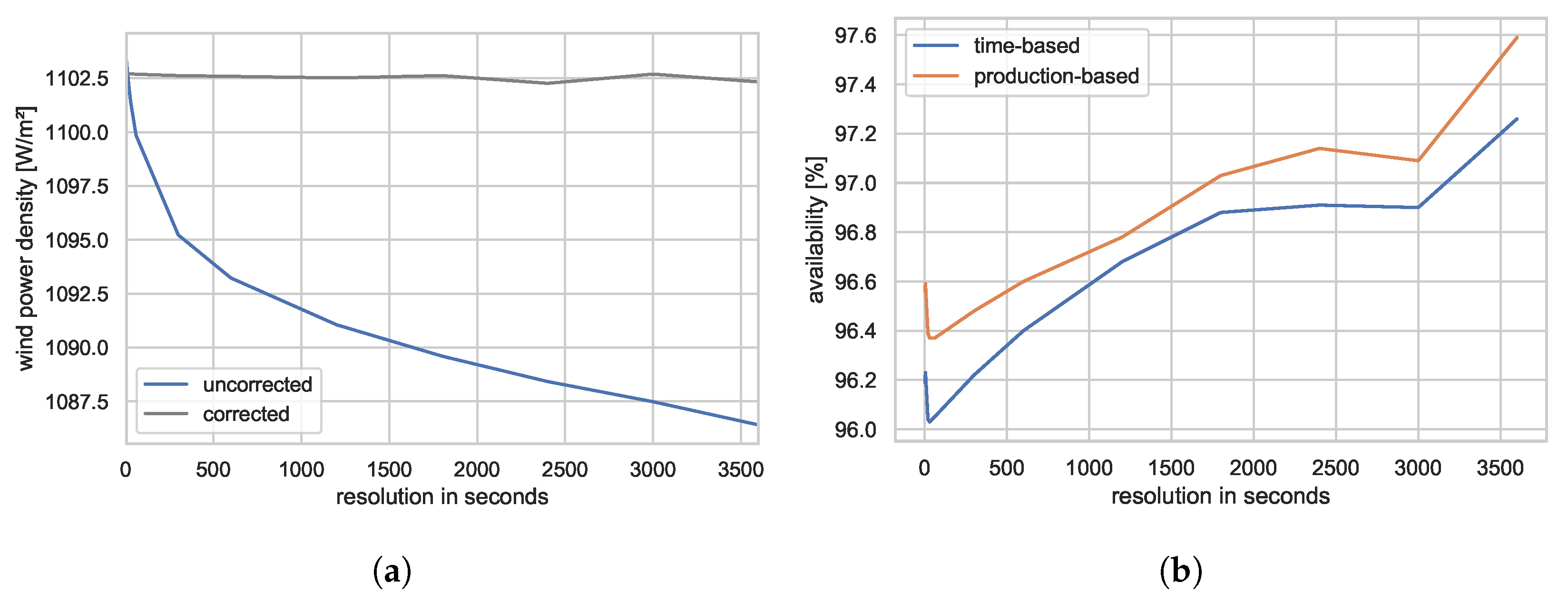
Equations of the second- or a higher-degree were affected by the smoothing effect. Missing information on extreme values led to lower KPI results since losing higher values has a greater impact than losing lower values. For the wind power density, one can correct this systematic deviation if the standard deviation of the wind speed is available, see Figure 3a. The correction assumes a normally distributed wind speed within the aggregation period as used to describe wind speed turbulences [31]. Of note, this is only valid for short periods. Long term wind speed distributions are generally characterized by Weibull or Rayleigh distributions. The correction algorithm showed an uncertainty of ~0.1% for the investigated examples since this assumption is not always met. This is still fifteen times lower than the observed systematic deviation when switching from 1 Hz data to hourly data.

The smoothing effect also affected the calculation of empirical power curves. Systematic deviations were witnessed in the transition area to the rated power, where high resolutions show a kink while lower resolutions smooth the transition and give the power curve its expected look. The IEC standard 61400-12-1/2 [30,31] requires 10 min data for empirical power curves. Different data resolutions led to deviations in the power curves and thus uncertainties when calculating energy yields. A relative standard deviation of approximately 0.4% was observed when calculating potential annual energy productions using power curves based on different resolutions over various wind speed distributions. Although this result should not be considered to be generally valid, its order of magnitude is expected to be correct.

This uncertainty also propagates into the calculation of the potential energy yield when assessing the production-based availability, but can be neglected due to its low impact. Much more important is the effect shown in Figure 3b. Initiatives such as the WInD-Pool, derive downtimes from wind speed and power measurements because distinct event information is often times missing. Although high-resolution data allows a clear distinction between operating times and standstill, this distinction becomes blurred at lower resolutions. The high-resolution area of Figure 3b shows a dropping in availability. This behavior can be explained by the assimilation of time steps adjacent to downtime because the negative power of several non-operational time steps can negate the positive power of single time steps. As the resolution further decreases, this behavior reverses. Short downtimes, such a five min-long reset of a WT, disappear in 10-min data. Of course, the behavior depicted in Figure 3b strongly depends on the distribution and length of downtimes, but the overall message is clear: Deriving downtime events from operational data is afflicted with significant uncertainties. Instead, distinct event information should be used whenever possible.

5.2. Data Availability

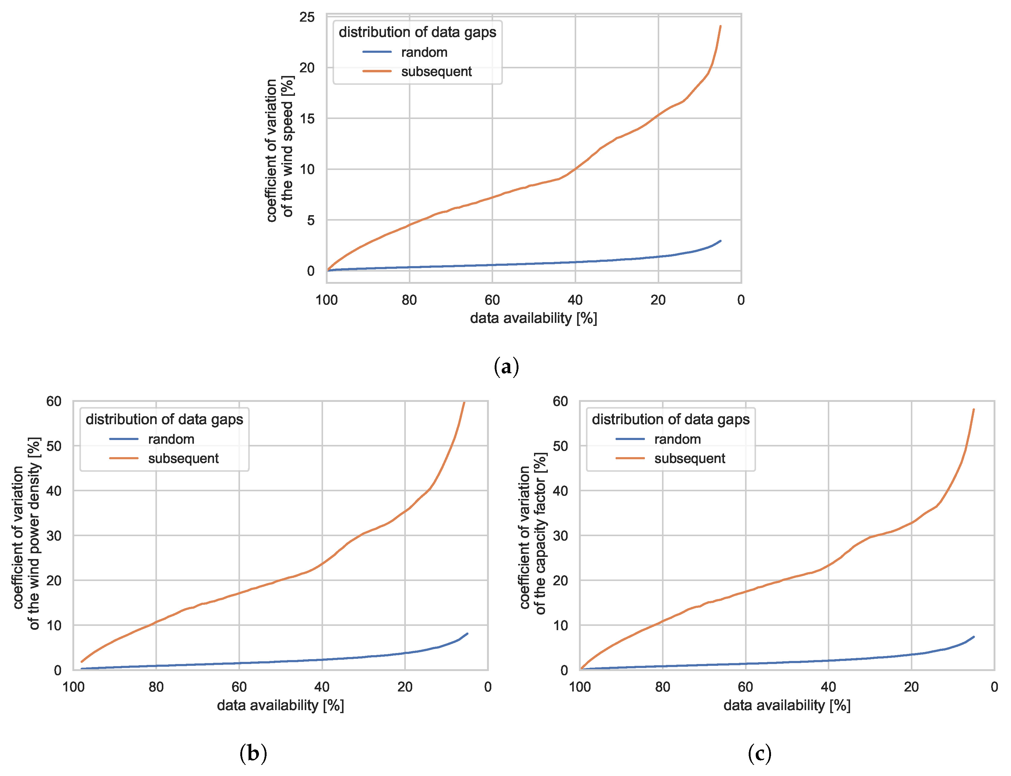
All considered KPIs are affected by decreasing data availabilities since the data is less representative of the considered period. Figure 4 shows the coefficient of variation in the results for (a) the wind speed, (b) the wind power density, and (c) the capacity factor, depending on the data availability and compared to a reference value based on a 100% data availability. The coefficient of variation was chosen over the standard deviation to make different datasets comparable.

The results illustrate that data availability is not the decisive factor, but rather the representativeness of the remaining data. Although the data availability is equivalent, short and random data gaps show only a minuscule effect, but long and subsequent data gaps lead to high uncertainties. Hereby, the results also emphasize the need of an entire year of measurements if representative results are to be achieved. The two depicted data gap distributions represent the best- and worst-case scenarios. For mixed experiments of shorter and longer data gaps, the coefficient of variation is expected to be between both cases.

A metric for the quality or representativeness of the remaining time series is needed to estimate case-specific uncertainties for data gap distributions witnessed in the field. Different attempts of the authors as well as existing metrics, such as the work of Bertino [53], did not lead to satisfying results or were not applicable for the described case. Thus, there is need for further research. As for the data resolution (Section 5.1), KPIs with a nonlinear relation to the wind speed measurement show a higher sensitivity to decreasing data availability. When comparing the results for the wind speed (Figure 4a) to the wind power density (Figure 4b) and the capacity factor (Figure 4c), the coefficient of variation is more than twice as high.

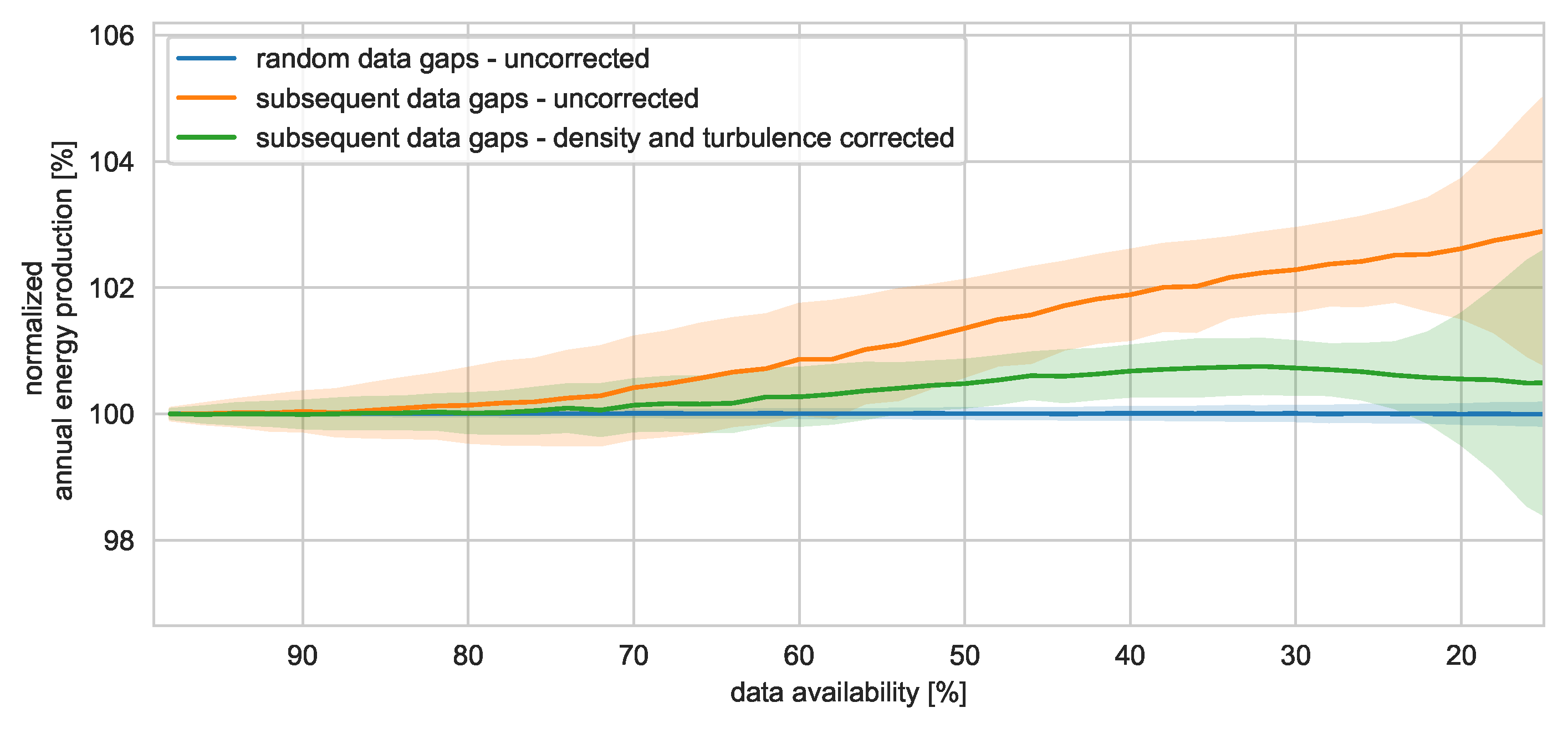
Even though the power curve of a WT represents the relation between two measurements (wind speed and power) and should not be affected by data gaps, the experiments carried out in this work showed increasing uncertainties with decreasing data availabilities, see Figure 5. Still, the uncertainties are much lower compared to the examples in Figure 4. If the data gaps are randomly distributed, the uncertainty of the resulting annual energy production is even for a data availability of just 20% below 0.2% and thus negligible. Subsequent data gaps cause not only considerably higher aleatoric uncertainties but also systematic deviations. These uncertainties can be mainly related to seasonal effects, such as varying air densities and turbulence intensities. By correcting the power curves for both effects [31,54], the uncertainties can be significantly reduced. At a data availability of 80%, the uncertainty for subsequent data gaps can be reduced from approximately 0.6% to 0.3%. However, some systematic uncertainties remain, and long data gaps should be avoided whenever possible. Even though the uncertainties caused by random data gaps could be only slightly decreased, it is highly recommended to perform a density and turbulence correction of power curves in any case. Figure 4 also highlights the need for a comprehensive data set for power curve assessments. Less than three months of data (here 25% data availability) cause an increasing uncertainty as the wind speed range is not sufficiently covered in many cases. Again, the order of magnitude of the above values is considered valid, while the concrete uncertainties can vary for other datasets. If an empirical power curve is used to calculate the production-based availability, its uncertainty propagates into the yield loss calculation.

5.3. Data Completeness

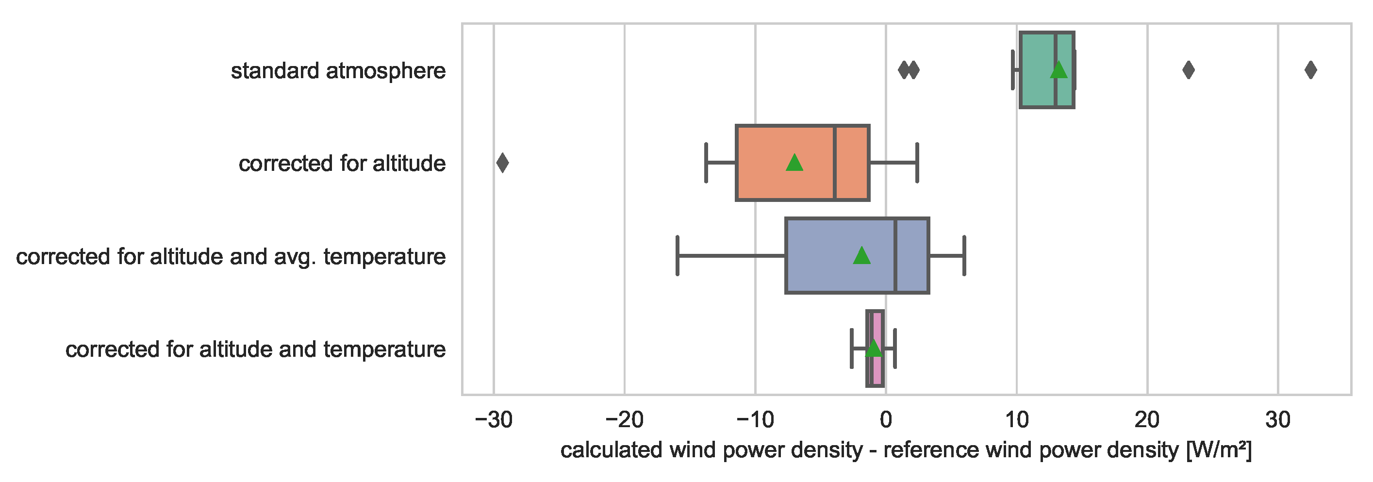
The importance of complete inputs for the calculation of KPIs is discussed in this section using the example of an air density measurement. Figure 6 shows the impact of the missing air density measurement and the quality of different approximations on the calculation of wind power density. If no air density measurement is available, it is common to use the standard atmosphere of 1.225 kg/m³. If the considered site or nacelle is at a higher altitude, this assumption leads to systematic high results. A correction for altitude likely results in an underestimation since the average temperature is usually below the standard temperature of 15 °C. If the air density is also corrected for the average temperature, a yearly wind power density KPI is already close to the reference as lower and higher temperatures balance out. Good results and drastically reduced deviations are achieved when temperature measurements are available.

If the small and systematic underestimation of the air density is ignored, the remaining deviations can be explained by weather-related pressure fluctuations. Thus, the uncertainty of an approximated air density can be derived from a known and site-specific distribution of the air pressure. As the sensitivity of the air density to changes of the humidity is low, the recommendation of the IEC standard 61400-12-1/2 [30,31] to use a default humidity of 50% is reasonable.

The presented results are validated against the North Sea WF data. The higher weather-related standard deviation of air pressure at the offshore location led to a higher standard deviation of the air density and thus of the wind power density. The discussed uncertainty propagates through the power curve to the production-based availability.

6. Discussion

This paper evaluates the sensitivity and uncertainty of five different KPIs to three different uncertainty causes related to data handling. Section 5 presents the most relevant findings of this work. A summary of the effect of each uncertainty cause on each KPI is provided in Table 1.

Furthermore, the following list provides a summary of key statements and recommendations for the discussed uncertainty causes and KPIs. It is intended to make the reader aware of potential pitfalls and sources of error and uncertainty in the day-to-day work with KPIs.

Data Resolution

• The mean wind speed and capacity factor are not affected by the data resolution.
• The systematic influence on the mean wind power density is caused by its cubic equation. By using the standard deviation of the wind speed, it can be corrected to an uncertainty of about 0.1%.
• By filtering the data thoroughly, effects on the power curve can be reduced to an acceptable level. The standard deviation of the resulting energy yields can be estimated at 0.4%.
• Whenever downtime events are derived from operational data, the number and length of downtime events heavily depend on the chosen data resolution. Availability metrics are affected accordingly. Thus, discrete event information should be used whenever possible. The production-based availability is furthermore affected through the power curve.

Data Availability

• The effect of decreasing data availability mainly depends on the distribution of data gaps in the whole dataset. While keeping the data availability constant, continuous data gaps cause much higher deviations than short and randomly distributed gaps. This emphasizes the need to use a full year of measurements if representative results are to be achieved. If data gaps are entirely random, the deviations can be almost neglected, and low data availabilities provide valid results.
• All discussed KPIs are affected by decreasing data availability. KPIs with a cubic equation, like the capacity factor or wind power density, show a higher sensitivity than the mean wind speed, which has a linear dependence. Site-specific simulations are necessary to quantify uncertainties.
• Short and random data gaps are of low importance when calculating the power curve. In contrast, long and continuous data gaps cause significant and systematic deviations and uncertainties, which can only be partially corrected.

Data Completeness

• Missing measurements of the air density or air pressure result in considerable deviation in the mean wind power density and power curve.
• The air density can be well approximated by a correction to the location altitude and the measured ambient temperature. The weather-related fluctuation of the air pressure leads to an uncertainty of about 0.013 kg/m³.
• Measuring the ambient humidity is only of little additional use. It can be assumed to be 50%.
• When approximating the air density, the uncertainty of the mean wind power density is approximately 1 W/m². At high wind speeds, this value may be higher.
• If a density correction of the wind speed is carried out based on an approximated air density, the corresponding uncertainty of the calculated power curve leads to an uncertainty of about 0.25% when calculating annual energy yields.

The results show that KPIs are affected by differing approaches and carefulness in data handling. In many cases, the resulting KPI uncertainties can be significantly reduced by simple measures, and the KPIs remain reliable. These are mostly systematic or epistemic uncertainties that can be largely corrected by additional effort. However, there are also substantial aleatoric uncertainties that depend, among other things, on the location and weather conditions but also on technical specifications and the operational behavior of WTs.

The present work provides a quantification of the uncertainties wherever possible. However, uncertainties vary with site- and technology-specific conditions in many cases. These results cannot be generalized and require specific simulations for valid uncertainty quantification. Regardless, the presented results can be used to estimate the magnitude and relevance of the uncertainties.

As shown in Section 3, there are additional potential causes for KPI uncertainties. Some of them are already part of previous publications and standards, while others require further research. Although this work covers the most important KPIs, there are many additional KPIs that could be of interest in the future. The mechanisms to simulate and test data handling-related uncertainties remain unchanged, and can be easily applied to additional KPIs. Furthermore, there is a need for additional research to quantify uncertainties due to decreasing data availability. A data quality index is required to describe the randomness and length of data gaps used to estimate the corresponding uncertainties more precisely. The current results provide a best- and worst-case scenario, which represent a starting point for future work.

To consider KPI uncertainties in daily work, there is a need to incorporate the corresponding calculations and visualizations into operational management and business intelligence systems. As shown by the IEC standard 61400-12-1/2 [30,31] as a best practice example, guidelines to combine various uncertainty causes and default values need to be agreed upon.