Featured Application
The developed software facilitates the quick calculation of magnetic flux density produced by electric current in facilities in whichever conditions, which can be used to detect inadmissible levels of immission and to propose design improvements.
Abstract
The World Health Organization (WHO) warns that the presence of magnetic fields due to the circulation of industrial frequency electrical currents may have repercussions on the health of living beings. Hence, it is crucially important that we are able to quantify these fields under the normal operating conditions of the facilities, both in their premises and in their surroundings, in order to take the appropriate corrective measures and assure the safety conditions imposed, in force, by regulations. For this purpose, CRMag® software has been developed. Using the simplified Maxwell equations for low frequencies, CRMag® calculates and represents the magnetic flux density (MFD) that electrical currents produce in the environment. Users can easily model electrical facilities through a friendly and simple data entry. MFDs calculated by CRMag® have been validated in real facilities and laboratory tests. With this software, exposure levels can be studied in any hypothetical scenario, even in inaccessible zones. This allows designers to guarantee that legal limits (occupational, general population, or precautionary levels related to epidemiological studies) are fulfilled. A real case study has been described to show how the reconfiguration of conductors in a distribution transformer substation (DTS) allows significant reductions in MFD in some points outside the facility.
1. Introduction
The influence of extremely low frequency (ELF) electromagnetic fields on the health of living beings, particularly humans, is a fact that raises interest and controversy in the scientific community and some concerns among many citizens. Possibly, the report that had the greatest worldwide impact and that raised the alarm was the so-called Karolinska report, published in 1993 by Feychting and Ahlbom [1], researchers at the prestigious Karolinska Institutet in Sweden. Although it is not the first scientific study on the subject [2], the large number of cases studied and the rigor of the method made it unique, and it is considered a basic reference in many countries. The report warns of a verified risk of cases of leukemia in children living next to high-voltage lines where the magnetic flux density (MFD) exceeded 0.2 µT.
Other researchers have tried to verify this influence with diverse results [3,4,5,6]. The same authors of the aforementioned report carried out a bibliographic review several years later [7] in which the main conclusion was that there is some evidence of a risk factor with an average value of 2 on this childhood disease that has a low incidence in the whole population. This risk is verified at locations where the average value of exceeds the threshold of 0.4 µT. This conclusion led the International Commission on Non-Ionizing Radiation Protection (ICNIRP), an independent organization with a great international prestige, to publish some recommendations on the general public’s exposure to electromagnetic fields [8], which were adopted by the World Health Organization (WHO) [9]. The established limits in these recommendations are based on the measurable phenomenon of induced currents in human organs. A threshold of 10 mA/m2 of current density was selected since lower values do not reveal health risks for humans. With regards to occupational exposure, this has been associated with an MFD of 500 µT at 50 Hz (or 420 µT at 60 Hz). For the general population, a safety factor of 5 is applied, resulting in an exposure limit of 100 µT at 50 Hz (or 83 µT at 60 Hz).
Subsequently, the Council of Europe adopted the same limits in [10], transcribed into Spanish legislation by [11].
The IEEE association also developed a standard on exposure limits to ELF magnetic fields [12].
For its part, the International Agency for Research on Cancer (IARC), based on the evidence presented in international research, classified the magnetic field of ELF as potentially carcinogenic (as opposed to the electric field) [13].
Numerous studies have tried to simulate or measure the physiological effects that ELF magnetic fields can produce inside the human body. In general, these studies analyze the induced current that the variable magnetic field can produce in various organs or tissues [14].
To date, the lack of evidence of a causal relationship between the ELF magnetic field and the development of certain diseases (such as leukemia) leads ICNIRP to consider that stricter mandatory limits cannot be established, such as 0.4 µT, beyond the recommendations given by this organization. However, it warns about the possible risk and suggests considering the precautionary measures that the WHO and other agencies have proposed. Based on this precautionary principle, some countries have set MFD immission limits below the values proposed by ICNIRP.
In [10], point 4 of the preamble states: "It is imperative to protect members of the general public within the Community against established adverse health effects that may result as a consequence of exposure to electromagnetic fields ". In line with this, recommendation VI says: “Member States, in order to enhance knowledge about the health effects of electromagnetic fields, should promote and review research relevant to electromagnetic fields and human health in the context of their national research programmes, taking into account Community and inter-national research recommendations and efforts from the widest possible range of sources”. In this sense, the Spanish government (as in other EU countries), with the regulation of high voltage electrical installations (RAT) [15], has imposed an obligation to study the magnetic fields produced by electrical installations to guarantee that the exposure limits regulated by [11] are not exceeded and to enhance the design of new facilities to minimize the magnetic field emissions. These studies would allow engineers to improve their knowledge about the possible incidence of magnetic fields produced by electrical facilities in the environment. The RAT establishes in the Complementary Technical Instruction (ITC) number 20 (ITC-RAT 20 Projects and preliminary projects) that the memory of high-voltage facility projects must include a study of magnetic fields in their surroundings.
It is necessary to have more information to improve the knowledge about the incidence of these fields on some diseases (such as childhood leukemia), as several authors explain in studies that try to improve the apparent correlation between the detected cases (which are very scarce) and the odds ratio (close to 2) that some epidemiological studies have obtained [16].
Some recent meta-analyses propose the thesis of a non-accidental correlation between the exposure to MFDs of more than 0.4 µT and the risk of childhood leukemia (odds ratio close to 2) or acute lymphocytic leukemia (odds ratio 2.43) [17]. Therefore, this value of 0.4 µT is often considered as a precautionary level for this disease. The need to deepen the analysis to achieve greater consensus is highlighted by many researchers [18].
Many recent studies try to correlate the risk of cancer and the proximity to high voltage lines [19,20]. To date, the results are still fairly uneven, although it seems that the proximity to these facilities increases the risk.
Other studies have tried to correlate the risk of cancer with the proximity to high-voltage underground lines, concluding that there is no increased risk in this case [21].
Additionally, some studies have also been conducted on the possible influence of the proximity to high voltage facilities on neurodegenerative diseases, but the results have not found any evidence [22].
There are not many recent advances about the cause effect relationship between magnetic fields and diseases. Nonetheless, the research remains active among the scientific community, as can be seen in [23,24].
One of the main disadvantages of epidemiological studies is the low number of individuals included in control areas and the low incidence that these diseases have on the general population. But there is an issue that has not been satisfactorily resolved to date: if the cause of the increased risk of certain diseases is the magnetic field (not the electric one), that effect should also be observed in locations where the magnetic field is produced by low voltage facilities. On the contrary, if the only measurable influence is observed in the proximity of high voltage lines, the cause cannot be attributed exclusively to the magnetic field.
Indeed, although both fields (magnetic and electric) are related by electromagnetic theory, at very low frequencies they are not coupled at the distances where people are exposed. In these cases, the magnetic field can be studied as a phenomenon that can be considered independent of the electric field of the system that produces it. In urban environments it is very common to find facilities such as distribution transformer substations (DTSs) next to inhabited buildings or very close to dwellings. As demonstrated in this paper, the MFD values that these facilities can produce on neighboring premises can be significantly higher than the threshold values of 0.4 µT. Therefore, extending an epidemiological analysis to these areas affected by the DTSs could considerably increase the number of people included in epidemiological studies.
The study of the magnetic fields produced by electrical installations can have a certain complexity. Due to this reason, sometimes, very simplified models are used for these studies. As a result of this simplification, only an indicative value can be provided, with a considerable margin of error (the fact that MFD is a vector quantity must be taken into account). Usually, actual values of MFD are considerably lower than the practical limit of 100 µT (1 G) that the regulation establishes for the general public at 50 Hz [10,11]. Therefore, an approximate calculation, even with a 100% error, can be used to justify this limit not being reached. The situation would be very different if the precautionary principle had been applied and that limit had been set at a lower value, like in Italy (3 µT is the limit for certain cases) and some other countries in Europe [25]. The tendency to reduce the size of DTSs, for example, in order to minimize their environmental impact [26], does not usually take into account aspects related to the emission of magnetic fields. In fact, the magnetic field is often reduced by shielding techniques [27], instead of studying the expected field before its execution and assessing other cheaper solutions. An example of a study of a shielding for a building located under high-voltage overhead lines is shown in [25]. However, the MFD in facilities is usually below the limits set by the regulation, as in [28].
An accurate calculation of the expected MFD produced by an electrical facility can provide useful information for several reasons:
- It increases the knowledge of this topic.
- It would provide guidance for the development of future standards.
- It enables the identification of the best installation practices and the rejection of inadequate assemblies.
- It facilitates the detection of overexposure in workers or the general population.
- The monitoring of exposure levels related to epidemiological studies can be carried out.
Nevertheless, given the complexity of this calculation, approximate prediction methods from the analysis of experimental measures are developed in some works [29]. For example, a simplistic numerical method for MFD prediction in open air type substations is shown in [30].
For this reason, in the Department of Electrical Engineering of the Universitat Politècnica de València, a software has been developed for the calculation of the MFDs produced by the electric currents in the facilities (CRMag®). This program has been designed to be easy to use by engineering firms when developing the projects of facilities. With this program, the geometric arrangement of conductors, their grouping, and so on, can be easily taken into account. This allows engineers to study optimal solutions that may provide significant reductions in MFDs. Thus, the influence of these facilities on neighboring premises, or on their environment, can be studied and minimized. The use of this type of software facilitates obtaining sufficient information about the influence of electrical installations on adjacent premises. This process is much simpler than measurement campaigns carried out by other researchers [31]. In addition, the information is more complete and reaches areas that are difficult access to carry out the measurements. Likewise, the simulation allows us to take into account scenarios that differ from the particular situation of the moment in which the measurement is carried out.
To demonstrate the usefulness of CRMag®, this paper includes a real case study of the expected magnetic field around a facility and the analysis of possible modifications in order to reduce the immission produced in neighboring premises.
This article begins with a brief summary of the physical principles involved in the calculation of the MFD produced by the electrical currents in Section 2. Then, Section 3 describes the simulation method with CRMag® and justifies the use of the developed software. Section 4 describes the case study selected for this study. It consists of the study of a real facility to optimize the arrangement of conductors in order to reduce the MFD emitted to neighboring premises. Then, Section 5 presents the results of the application of the developed software to the selected case study and a discussion of the obtained results. Finally, the conclusions of the developed work are presented in Section 6.
2. Physical Principles
The MFD created at point P by electric charge Q, which moves in vacuum with velocity , is:
where r is the vector from the charge to the point.
In the International System of Units (ISU) H/m o N/A2.
From this expression it is easy to obtain the MFD at point P created by an intensity that circulates through a filiform conductor:
Thus, for a rectilinear conductor of infinite length, the MFD created at point P, at distance r from the conductor, is a vector perpendicular to the plane defined by the conductor and point P, whose module is calculated using Biot and Savart’s Law:
Similarly, an analytical equation can be derived for a straight finite conductor.
These expressions can be used outside the conductor, not inside them. Nonetheless, this is not important for the study of the magnetic fields produced by the conductors of facilities in their neighborhoods.
Therefore, the MFD in P created by a circuit with a current I will be:
If there are k conductors covered by intensities , , …, , each one will create an MFD at P, , ,…,. These MFDs are vectors, so the total MFD will be:
If sinusoidal electric currents are considered, magnetic flux will also be a sinusoidal function. In this case, the effective value of the MFD at P must be computed. It may also be useful to know the components of along three orthogonal axes (X, Y, Z), which are called , and . These components may allow the identification of the source of the field that is measured at a certain point.
If a varying magnetic field crosses a metallic object, electromotive forces are induced in that object. As a consequence of these electromotive forces, electric currents flow through the object (Foucault or eddy currents). These currents heat the object. The induced currents, in turn, produce magnetic fields. Induced currents are opposed to the cause that produces them, so the resulting MFD tends to decrease, thus producing a shielding effect. Unless the metallic object is significantly thick, the magnetic shielding effect is weak. However, this effect is greater with screens of ferromagnetic materials.
In the case of a thin metal plate, close to the primary source of the magnetic field, disregarding the effect of the surface charge on the plate, the MFD produced by the eddy currents on a close point P will be:
where is the vector of eddy current density in the element , at the coordinates s(x,y,z) and , the vector from that element to point P. Due to the small thickness of the plate, it is admissible, in general, to consider it as a plane and convert equation (6) into a surface integral. The influence of this phenomenon depends on many factors (metal resistivity, the direction of the MFD inside the plate, and so on) and decreases when moving away from the plate. Experimentally, this effect can be taken into account with an MFD attenuation coefficient.
3. Materials and Methods
3.1. CRMag® Software for the Calculation of MFDs Produced by Electric Currents
The CRMag® software is a calculation tool developed with MATLAB at the University Research Institute for Energy Engineering (IUIIE) of the Universitat Politècnica de València, which was registered at the Research and Development Management Service of the aforementioned university, with registration number R-19161-2017—CRMag®. The purpose of this software is to calculate and represent the MFD produced by the circulation of currents in electrical facilities, using Equations (1)–(5), both in the premises where these installations are located and in their surroundings.
In order to do this, the different conductor straight sections are substituted by a discrete set of little linear elements. A grid of calculation points is defined by the user. For every calculation point in the selected grid, a numerical integration of Equation (4) is solved using the rectangle method for every conductor of every phase. For each phase, this integration is solved in the three Cartesian axes (X,Y,Z). After completing the integration of all the little elements, the phasor magnitudes calculated for every phase are temporally composed. The same applies to and . Finally, the root mean square value of B is computed.
As the rectangle method for numerical integration is not exact, the error will depend on the number of discrete little elements used for every conductor section. This can be adjusted by the user, thus increasing the accuracy of the calculations. When the MFD is calculated far from the wires, this error is negligible if the distance to them is much greater than the size of the selected elements. CRMag® has been specifically designed to study typical installations. For more complex situations there are other programs (such as CDEGS or XGSLabTM) that are more complex and powerful.
The program has two calculation modes. In the main mode, also called installations mode, the MFD produced by the electric currents in electrical facilities such as DTSs or electrical substations can be studied. In this mode, electrical conductors are represented by straight sections, considering the electrical shield if it is included (like in insulated cables). In the second mode, also called lines mode, the MFD produced by high-voltage overhead lines, considering the catenaries adopted by conductors and the currents that can be induced in earth wires, can be calculated and represented. The main screen of the installations mode is shown in Figure 1.
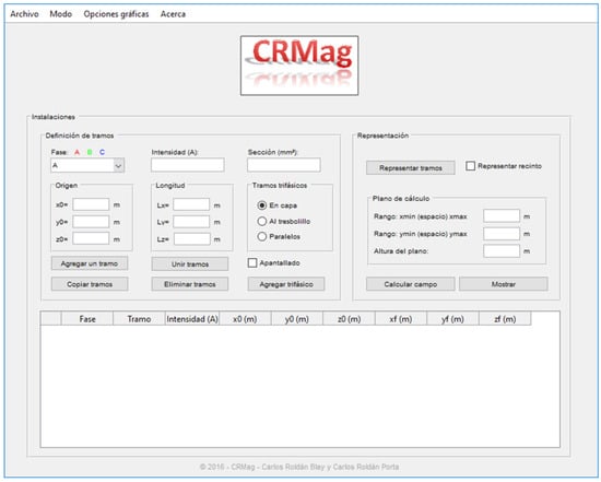
Figure 1.
Main screen of the CRMag® software.
To calculate the MFD produced by electric currents in a facility, the user must enter the geometric arrangement with the coordinates of every conductor section and their currents. The program can simulate both single-phase and three-phase installations with or without a neutral conductor.
The geometry of the defined installation and premises can be displayed to verify that everything is correct and proceed to calculate the MFD.
The MFD is always calculated in a horizontal plane at the desired height above the coordinate z=0, for example, 1 m. In that plane, a grid of equidistant points is drawn in which the MFD produced by all the currents of the installation is calculated.
The results can be represented as a three-dimensional surface or as two-dimensional curves produced by cutting the surface by fixing the value of coordinates x or y. The Z axis of the three-dimensional graphs corresponds to the calculated magnitude of B (in µT). This magnitude can be displayed using a scale different from those of the X and Y axes, which represent coordinates in m. The representation of B can be limited to a maximum value. This allows us to create graphs in which the part of the surface that exceeds a certain value is shown in a uniform color and a flat shape fixed to the maximum value to be represented. In this way, the contours of this area form an “isoflux” curve (a curve where the MFD has a determined constant value).
Two-dimensional graphics allow the user to get a quick overview of how the MFD is distributed along a path in the X or Y direction, for example, next to the edge of an installation (such us next to the facade).
With the resulting graphs, the user can study the magnetic field within an installation, in the surroundings (beyond the edges of the installation), or even in other neighboring areas, such as the upper or lower floors.
3.2. Comparison between the Measurement and Simulation of the MFD
The measurement of the MFD produced by low frequency variable currents can be done with electromagnetic field (EMF) meters. These devices use scanning coils or Hall-effect devices. Hall-effect devices can also be used in magnetometers, which allow us to measure a static magnetic field. EMF meters can perform measurements in one direction or in three orthogonal directions.
Using CRMag®, the circuit depicted in Figure 2, with an electric current of 7.69 A, has been simulated, calculating the MFD in a horizontal plane at 2.5 cm in height above the X–Y plane. The simulation results are represented in Figure 3.
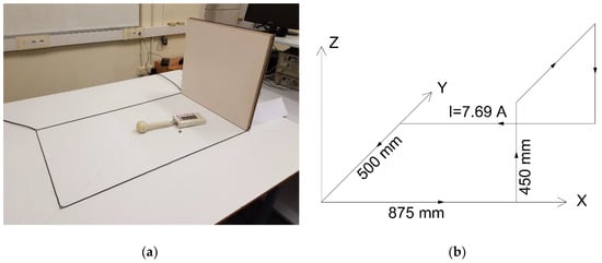
Figure 2.
(a) Simulated and measured circuit and (b) its 3D representation.
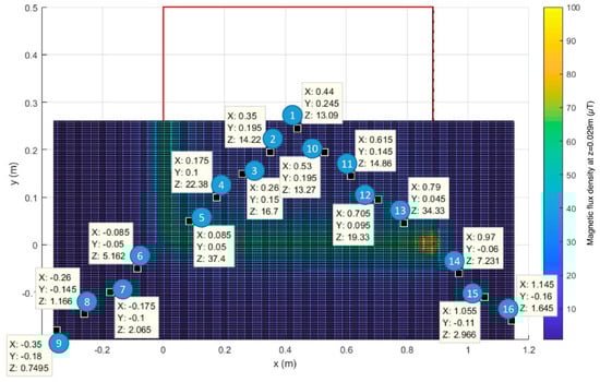
Figure 3.
Simulation of the test circuit.
The values calculated at points 1 to 16 indicated in Figure 3 are shown in Table 1, together with the values measured at the same points using a 3-axis meter (3D H / E fieldmeter ESM-100 Maschek). Figure 4 shows the results of the measurements (in blue) and those obtained by the simulation (in orange) in these points. In Table 2, some technical data about the mentioned field meter are shown.

Table 1.
Comparison of simulation and measurement results.
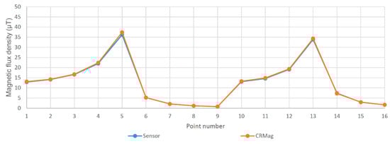
Figure 4.
Representation of simulation and measurement results.
Table 2.
Three-dimensional H/E fieldmeter ESM-100 Maschek technical data.
Table 1 and Figure 4 demonstrate the high level of accuracy achieved when using the developed software. The differences are due to small inaccuracies in the placement of the probe and the finite size of the probe, which makes the measured value an average of the MFD in a small region, but not a point value.
Therefore, in studies of the EMF produced by electric currents, the calculation results can be used with a high level of confidence instead of the measured data. The measurement requires more time, especially in the case where the user wants to get a complete view of the MFDs in a large area and not just a specific value. In addition, simulation allows the users to calculate MFDs in hard-to-reach areas or vary the values of the electric current in the conductors at their convenience, thus allowing them to analyze multiple scenarios, whereas measurements are representative only of the existing conditions in the circuits at the moment when the measurement is made.
Another important aspect to highlight the advantage of simulation in these studies is that it allows the user to analyze the effect of possible modifications of the facilities and thereby choose the arrangements or designs that have less influence on the environment. The case study described in detail in Section 4 shows some possibilities that simulation offers in the design stage of a new facility as well as in the study of the influence of existing facilities on nearby premises.
Since the described case study corresponds to a DTS, it is necessary to include the effect of the transformer to simulate the MFD. For this reason, the authors have made MFD measurements in several DTSs in order to achieve a simple model, but accurate enough to be used in CRMag® and avoid the use of complex finite element models.
Figure 5 shows a 630 kVA transformer. Figure 6 indicates the points where MFD measurements have been made, at a height of 1m above the ground.
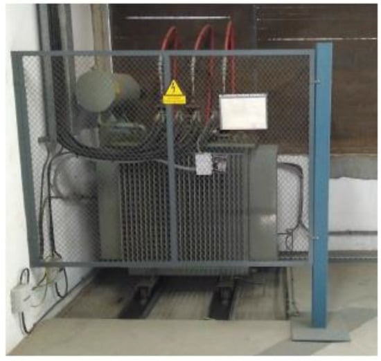
Figure 5.
Example of a distribution transformer studied to test the developed model.
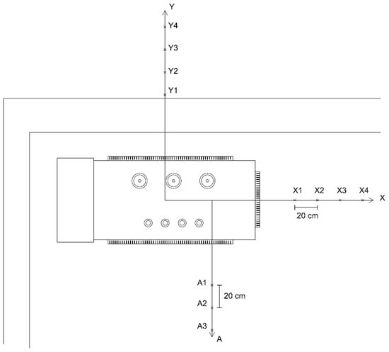
Figure 6.
Diagram of the studied distributed transformer and the points where the MFD has been measured.
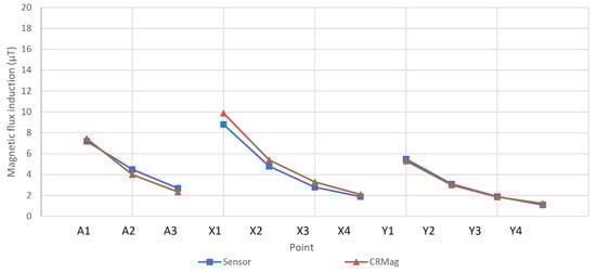
Figure 7.
Comparison between the measured and calculated magnetic flux density (MFD) around the distribution transformer.
As depicted in Figure 7, the MFD created by the transformer decreases very quickly as the distance to the machine increases. This fact and the need to maintain certain safety distances between the machine and the enclosure walls makes the influence of the transformer on neighboring premises small, in general. This influence is clearly lower than the influence of the low voltage power conductors. Therefore, in many cases, a good approximation is obtained by modeling only the cited wiring. Nonetheless, for this study, both effects will be added.
3.3. Analysis of MFD Emission Reduction
When designing a high voltage facility, trying to minimize the emission produced by an installation in its surroundings is convenient, whether in public spaces or in other premises. As mentioned above, this paper proposes the use of CRMag® as a quick and simple procedure to simulate the MFD produced in these areas with normal installation conditions. Then, using the same software, the user can study the alternative conductors or equipment layout by applying the following steps:
- Remove conductors from the edges of the premises (when possible).
- Minimize the distance between conductors of different phases.
- Balance the arrangement of conductors by alternating the phases.
The procedure to minimize the immission is described in Figure 8.
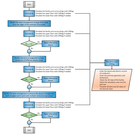
Figure 8.
Proposed method to study and minimize the immission in the surroundings of an electrical installation.
4. Case study
The calculation of the MFD produced by a real DTS in its surroundings has been selected as an example to show the application of the developed software. This example will be studied to demonstrate the importance of considering aspects such as the wires’ arrangement when executing the installation of the substation. This DTS is located on the ground floor of a building. Since a bedroom could exist on the upper floor, it is necessary to study the MFD about 20 cm above that floor. Using the program, the geometry of the room and the wiring have been introduced and the calculations have been made. The results of these calculations are shown in the following section. Then, analyzing the results, some simple modifications have been proposed to ensure the reduction in the MFDs around the substation. Figure 9 shows a picture of the studied DTS located in a building.
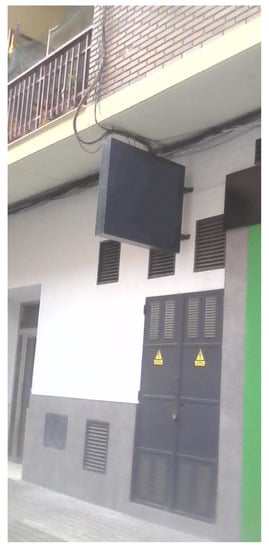
Figure 9.
Location of the studied distribution transformer substation (DTS) in a building.
The DTS (20,000 V/400 V, 630 kVA) has the following dimensions: 4 m in the direction of the X axis, 2.5 m in the direction of the Y axis and 2.5 m in height. Figure 10 shows the floor plan of the DTS and a 3D view. The high voltage line (20 kV) consists of three unipolar aluminum conductors (one for each phase) of 240 mm2 with high module ethylene–propylene (HEPR) insulation, with a 16 mm2 copper shield and Z1 type cover. This underground line approaches the center with a certain slope. Then, it continues parallel to the ground and arrives at the medium voltage switchgears, where it crosses them. Finally, it leaves parallel to its entry path (urban DTS in a ring main feeder). For this line, 250 A are assumed per phase. On the other hand, the low voltage line leaves the transformer terminals and goes up to a tray on the wall 2.2 m high. It is a line with three conductors per phase and an electric current of 300 A has been assumed in each conductor. After the tray with all the conductors arranged in a single layer, these go down, in contact with the wall, in groups of three (equilateral triangles with wires touching each other), passing through the low voltage panel. Then, the conductors are buried at 40 cm deep to go to the low voltage installation. The high voltage section that passes through the protection and measurement electrical cabinets and reaches the high voltage transformer terminals is not included in the study, as it has a very low current (about 20 A) and produces much lower MFD levels.
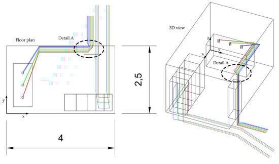
Figure 10.
Floor plan (left) and 3D view (right) of the DTS to study with the existing cable routing (dimensions in meters). Detail A is shown in Figure 11.
The geometry data and layout of the conductors have been entered in CRMag® to study the MFD produced by this facility. The definition of the whole model is developed in just a few minutes. The program automatically calculates the induced currents in the high voltage insulated cable shields (these are grounded according to a solid bonding scheme) and conveniently corrects the calculation of the MFD. For some elements, such as metallic electrical cabinets or transformers, the user can select an attenuation factor, taking their dimensions into account. With a preliminary calculation, the user can find which areas have higher MFD levels, to make a detailed study of them. In order to show here the results of greatest interest and propose an alternative that has a great impact on the results, the MFD will be studied on the upper floor and on the sidewalk of the main facade, where the line enters and leaves the facility.
For the immission study on the upper floor, the calculation height is the plane at z=2.9 m, taking into account the 2.5 m in height of the DTS, plus 20 cm of floor thickness and calculating 20 cm above the floor. This is done because there could be a bedroom in the existing dwelling. This calculation will be carried out on the entire upper floor in a 4-m-wide square (from the coordinate x=0, y=0 to the coordinate x=4, y=4).
For the study of the MFD produced on the sidewalk of the main facade, the MFD will be studied at a height of 1 m above the ground from the coordinate x=0, y=2.6 (a wall thickness of 10 cm is assumed) to the coordinate x=4, y=4.
The calculation plane mesh has been plotted with points every 10 cm in the directions of both axes (X and Y). A simulation with 400 wire sections, using a calculation grid with 1600 points and using 100 discrete elements per section takes 36 seconds.
After analyzing the obtained results, which are shown in the next section, the study is repeated using an alternative conductors’ layout, which shows much lower immission levels for this case. Other paths have been tested and intermediate MFD values between the studied scenarios have been obtained. The new proposal is to group conductors mixing the different phase. Among all the existing possibilities, the one that produces the least MFD has been chosen. In this way, along the tray, the original phases sequence of the nine conductors, 0-0-0-4-4-4-8-8-8, will be compared to the proposed one, 0-4-8-8-0-4-4-8-0. In the same way, in the wiring harness that goes down the wall, the conductors will be arranged so that each triplet has one cable of each phase. In addition, each triplet will be a transposition of the previous triplet in order to minimize the induction produced in the surroundings. This distribution of the different conductors of each phase will produce greater compensations between them than the original one, due to the better-balanced distances to the calculation points. Therefore, the proposed alternative will produce smaller MFDs. In this way, the phases’ sequence in the triplets (following the X-axis direction) will change from the original one, 8-8-8-4-4-4-0-0-0, to the proposed alternative, 4-0-8-0-8-4-8-4-0. Figure 11 shows a detail of both cases in these zones, extracted from the CRMag® software. The isolated conductors are placed in different order in the new alternative, as shown in Figure 11b. This Figure is a schematic representation obtained from the software. Nonetheless, all conductors are insulated and they do not touch each other. Finally, the buried cables that leave the center towards the low-voltage facility will have the same arrangement as the one used along the tray.
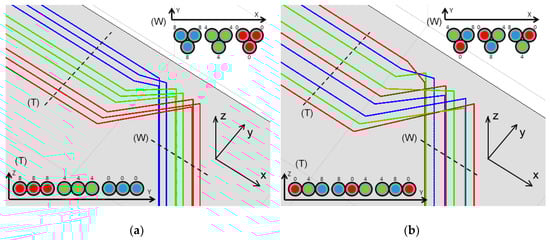
Figure 11.
Original conductors’ layout (left) and the proposed alternative (right). This is the detail A of Figure 10 for both alternatives. The axes directions are indicated in the figure.
After studying both cases, the highest MFDs will be compared by making some cuts for a fixed value of the y-coordinate or the x-coordinate. The curves of both alternatives will be represented to draw conclusions. The rest of the alternatives studied, consisting of the transpositions of the selected alternative, have been rejected since they do not provide any improvement.
5. Results and Discussion
The result of the calculation of the MFD at a height of 20 cm above the upper floor is shown in Figure 12.
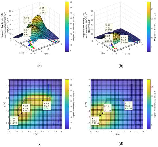
Figure 12.
MFD on the upper floor in 3D using (a) the original layout and (b) the proposed alternative. MFD on the upper floor in 2D using (c) the original layout and (d) the proposed alternative.
In the 3D graphs of Figure 12, the value of the z-coordinate corresponds to MFD B. In this figure, the points with the greatest MFD have been highlighted. In the original case, these correspond to those that remain above the axis of the tray. It is observed that the highest MFD is 50.27 µT at x=2.5 m and y=2.3 m. This value is higher than 50% of the reference levels in the regulation. The calculation results are also shown in Figure 12, using the proposed optimal alternative of cable arrangement. In this case, the highest MFD 28.85 µT is above the transformer. However, in the area that previously had the highest values, a maximum of 8.53 µT are calculated with the proposed alternative. Therefore, a reduction of 80.03% is obtained near the modified section.
To analyze in greater detail the magnetic field in the worst areas, a cut can be made at y=2.3 m or at x=1.2 m to represent the resulting two-dimensional curves by keeping one coordinate fixed. In these two-dimensional graphs, the Y axis values correspond to B and the X axis values correspond to the non-fixed coordinate (x or y). In Figure 13a, this curve is shown for both proposals at y=2.3 m. Similarly, Figure 13b represents these curves at x=1.2 m. As depicted in Figure 13, there is a wide area with larger MFDs in the original scenario than in the proposed alternative. The obtained reductions are quite significant in some areas. On the other hand, these reductions are not so significant in farther areas.
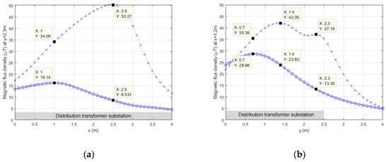
Figure 13.
MFD on the upper floor at a height of 20 cm (z=2.9 m), at y=2.3m (a), and at x=1.2m (b) for the original situation (crosses) and for the proposed alternative (circles).
Logically, the area above the tray and the cables that go down in triplets has a larger MFD because the conductors are closer to the calculation plane. However, in the original case, there is another important fact to take into account that causes the MFD to be so high. In the original situation, a decompensation takes place because the distances between the conductors of the different phases and the calculation points are not balanced. That is, for a given point in the calculation plane, the distance to the cables of one phase is not very similar to the distance to the cables of the other phases. Thus, one way to reduce the MFD in this studied area is to lay the nine conductors, alternating the different phases, as proposed in this study. Therefore, for a given point in the studied plane, the average distance to the cables of each phase is very similar, since they are better distributed. Consequently, the MFD produced by each phase is compensated with the MFD produced by the others, and the MFD is considerably reduced.
In the area above the transformer, the reduction is much smaller because these conductors are farther away from the calculation plane and because the phases are separated and minor changes can be proposed. Additionally, the effect of the transformer is the same in both cases. To verify this, the resulting MFD curves at x=1.2 m are shown in Figure 13b.
If the field on the sidewalk next to the main facade is studied, the influence of alternating phases can also be significantly noticed. For this purpose, the MFD is calculated outside at a height of z=1 m, from the coordinate x=0 m, y=2.6 m (a wall thickness of 10 cm has been assumed) to the coordinate x=4 m, y=4 m. Figure 14 shows the MFD for both cases, in 3D and in 2D, highlighting the highest values.
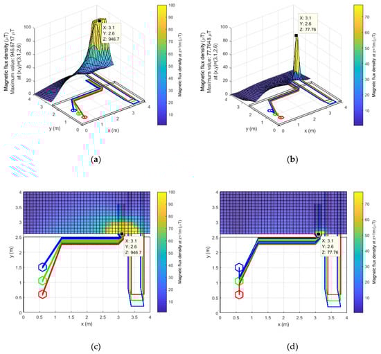
Figure 14.
MFD on the sidewalk in 3D using (a) the original layout and (b) the proposed alternative. MFD on the sidewalk in 2D using (c) the original layout and (d) the proposed alternative.
In order to represent the 3D graphic, the MFD has been curtailed to a limit value of 100 µT, since in the original case there was a maximum value of 946.7 µT that made it impossible to visualize the shape of the represented surface. In Figure 15a, a cut of the MFD calculated at y=2.7 m is shown (10 cm from the facade) to compare the MFD along the entire center facade in both scenarios. A similar curve is shown in Figure 15b, but 20 cm from the facade (y=2.8 m).
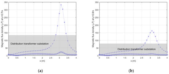
Figure 15.
MFD on the sidewalk at a height of 100 cm (z=1 m) at y=2.7m (a) and at y=2.8m (b) for the original situation (crosses) and for the proposed alternative (circles).
As shown in Figure 15, the maximum MFD at y=2.7 m has been reduced from 332 µT to a value of 23.47 µT, which represents a reduction of 92.93%. In addition, the reduction is significant along the whole facade. Furthermore, the alternative configuration does not produce values of 100 µT or higher at any point outside the DTS.
6. Conclusions
Several epidemiological studies consistently warn of a risk with respect to certain diseases (such as childhood leukemia, with odds ratios close to 2) in people living close to high voltage lines, where MFDs greater than 0.4 µT are presented. This has led to the consideration of the magnetic field as potentially carcinogenic by international organizations such as the IARC. The European authorities warn of this risk and promote research in this area in order to improve their knowledge [10].
In Spain, as in other countries of the European Community, the study of the magnetic field produced by high voltage electrical facilities is mandatory, as stated in the High Voltage Electrical Installations Regulation [15].
This work describes a new software called CRMag®. It is a simple but powerful tool for the calculation and three-dimensional representation of the magnetic field produced by the circulation of currents in electrical facilities.
This software has been designed to facilitate the data entry for electrical installations using graphical user interfaces and simple forms. The calculation is carried out quickly and the results are always shown graphically and numerically. The results have been designed to be easy to understand and include in reports and studies.
The software has been validated by numerous checks in real facilities and by laboratory tests.
The main advantages of the use of such software are:
- It requires less time than measuring.
- It allows the user to simulate different alternative layouts of conductors easily.
- It allows the user to simulate the facility with the desired conditions, regardless of the actual currents.
- The simulation allows the user to represent the MFD on a wide area, meaning that it is very simple to study safety distances to the facility.
- Occupational or general public overexposure in relation to regulated limits can be prevented. In the same way, precautionary levels related to childhood leukemia and other diseases can be checked.
- CRMag® is an affordable tool specifically designed to calculate MFDs in electrical installation. It facilitates the definition of typical installations.
The presented software allows the user to study the magnetic field of an existing installation or to anticipate its expected magnitude when a new installation is projected. In this way, it is easy to study alternatives to minimize the impact of the designed facility on neighboring premises or locations. In this work, a case study has been described to show the different results that the software produces and to study alternatives to reduce the immission of an installation on the neighboring areas.
Thanks to a study that was carried out, an alternative design has been found that reduces the maximum MFDs in certain areas to values more than 80% lower than the MFDs produced by the initial design.
This case study has been selected to prove the great influence of the arrangement of the conductors of different phases when the lines are installed. In the presented case study, the optimal sequence of phases to lay conductors in the tray and on the wall (by triplets) is shown. The data provided in the case study are of great interest to engineers related to the project of constructing this type of facility. Additionally, the improvements shown in this case are obtained with simple simulations and can be easily implemented.
The knowledge of the MFD produced by facilities can be of great help in future research about the real influence that this type of pollution has on the development of certain diseases. Therefore, we cannot dismiss the notion that future regulations stating lower limits regarding the exposure of people to this type of influence will be an eventual result of new research.
Finally, the developed calculation tool can also be very useful for research centers that carry out studies related to the MFD produced by conductors of a facility.
7. Patents
The authors registered the developed software “CRMag®: Programa de cálculo y representación de campos magnéticos en instalaciones eléctricas” with the reference number R-19161-2017 on February 14, 2017, in Spain.
Author Contributions
Conceptualization, C.R.-B. and C.R.-P.; Data curation, C.R.-B. and C.R.-P.; Formal analysis, C.R.-B. and C.R.-P.; Investigation, C.R.-B. and C.R.-P.; Methodology, C.R.-B. and C.R.-P.; Resources, C.R.-B. and C.R.-P.; Software, C.R.-B. and C.R.-P.; Supervision, C.R.-B. and C.R.-P.; Validation, C.R.-B. and C.R.-P.; Visualization, C.R.-B. and C.R.-P.; Writing–original draft, C.R.-B. and C.R.-P.; Writing–review & editing, C.R.-B. and C.R.-P. All authors have read and agreed to the published version of the manuscript.
Funding
This research received no external funding.
Acknowledgments
This work has been possible thanks to the support of the Universitat Politècnica de València.
Conflicts of Interest
The authors declare no conflict of interest.
Abbreviations
| DTS | distribution transformer substation |
| ELF | extremely low frequency |
| EMF | electromagnetic field |
| HEPR | high module ethylene-propylene |
| IARC | International Agency for Research on Cancer |
| ICNIRP | International Commission on Non-Ionizing Radiation Protection |
| ISU | International System of Units |
| ITC | Complementary Technical Instruction |
| IUIIE | University Research Institute for Energy Engineering |
| MFD | Magnetic flux density |
| RAT | Regulation of high voltage electrical installations |
| WHO | World Health Organization |
References
- Feychting, M.; Alhbom, M. Magnetic Fields and Cancer in Children Residing Near Swedish High-voltage Power Lines. Am. J. Epidemiol. 1993, 138, 467–481. [Google Scholar] [CrossRef] [PubMed]
- Wertheimer, N.; Leeper, E. ELECTRICAL WIRING CONFIGURATIONS AND CHILDHOOD CANCER. Am. J. Epidemiol. 1979, 109, 273–284. [Google Scholar] [CrossRef] [PubMed]
- Green, L.M.; Miller, A.B.; Villeneuve, P.J.; Agnew, D.A.; Greenberg, M.L.; Li, J.; Donnelly, K.E. A case-control study of childhood leukemia in southern Ontario, Canada, and exposure to magnetic fields in residences. Int. J. Cancer 1999, 82, 161–170. [Google Scholar] [CrossRef]
- Green, L.M.; Miller, A.B.; Agnew, D.A.; Greenberg, M.L.; Li, J.; Villeneuve, P.J.; Tibshirani, R. Childhood leukemia and personal monitoring of residential exposures to electric and magnetic fields in Ontario, Canada. Cancer Causes Control. 1999, 10, 233–243. [Google Scholar] [CrossRef]
- McBride, M.L.; Gallagher, R.P.; Theriault, G.; Armstrong, B.G.; Tamaro, S.; Spinelli, J.J.; Deadman, J.E.; Fincham, S.; Robson, D.; Choi, W. Power-frequency electric and magnetic fields and risk of childhood leukemia in Canada. Am. J. Epidemiol. 1999, 149, 831–842. [Google Scholar] [CrossRef]
- Tynes, T.; Haldorsen, T. Electromagnetic Fields and Cancer in Children Residing Near Norwegian High-Voltage Power Lines. Am. J. Epidemiol. 1997, 145, 219–226. [Google Scholar] [CrossRef]
- Ahlbom, A.; Day, N.; Feychting, M.; Roman, E.; Skinner, J.; Dockerty, J.; Linet, M.; McBride, M.; Michaelis, J.; Olsen, J.H.; et al. A pooled analysis of magnetic fields and childhood leukaemia. Br. J. Cancer 2000, 83, 692–698. [Google Scholar] [CrossRef]
- ICNIRP 2010 International Commission on Non-Ionizing Radiation Protection. Guidelines for limiting exposure to time-varying electric and magnetic fields (1 Hz to 100 kHz). Health Phys. 2010, 99, 818–836. [Google Scholar] [CrossRef]
- World Health Organization—Electromagnetic Fields and Public Health. Exposure to Extremely Low Frequency Fields. Available online: https://www.who.int/peh-emf/publications/facts/fs322/en/ (accessed on 8 January 2020).
- Council Recommendation 1999/519/EC of 12 July 1999 on the limitation of exposure of general public to electromagnetic fields (0 Hz to 300 GHz). Off. J. Eur. Commun. L 199 1999, 30, 59–70.
- Boletín Oficial del Estado. Real Decreto 1066/2001, de 28 de Septiembre, por el que se Aprueba el Reglamento que Establece Condiciones de Protección del Dominio Público Radioeléctrico, Restricciones a las Emisiones Radioeléctricas y Medidas de Protección Sanitaria Frente a Emisiones Radioeléctricas, (in Spanish), 2001. Available online: https://www.boe.es/buscar/pdf/2001/BOE-A-2001-18256-consolidado.pdf (accessed on 8 January 2020).
- IEEE Standard for Safety Levels with Respect to Human Exposure to Electromagnetic Fields, 0–3 kHz. IEEE-SASB Coord. Comm. 2008. [CrossRef]
- International Agency for Research on Cancer Classifies Radiofrequency Electromagnetic Fields as Possibly Carcinogenic to Humans, World Health Organization, Lyon, 2011. Available online: https://www.iarc.fr/wp-content/uploads/2018/07/pr208_E.pdf (accessed on 8 January 2020).
- Kavet, R.; Dovan, T.; Reilly, J.P. The relationship between anatomically correct electric and magnetic field dosimetry and publishedelectric and magnetic field exposure limits. Radiat. Prot. Dosim. 2012, 152, 279–295. [Google Scholar] [CrossRef][Green Version]
- Boletín Oficial del Estado. Real Decreto 337/2014, de 9 de Mayo, por el que se Aprueban el Reglamento Sobre Condiciones Técnicas y Garantías de Seguridad en Instalaciones Eléctricas de Alta Tensión y sus Instrucciones Técnicas Complementarias ITC-RAT 01 a 23, (in Spanish), 2014. Available online: https://www.boe.es/boe/dias/2014/06/09/pdfs/BOE-A-2014-6084.pdf (accessed on 8 January 2020).
- Kheifets, L.; Afifi, A.; Monroe, J.; Swanson, J. Exploring exposure–response for magnetic fields and childhood leukemia. J. Expo. Sci. Environ. Epidemiol. 2011, 21, 625. [Google Scholar] [CrossRef][Green Version]
- Zhao, L.; Liu, X.; Wang, C.; Yan, K.; Lin, X.; Li, S.; Bao, H.; Liu, X. Magnetic fields exposure and childhood leukemia risk: A meta-analysis based on 11,699 cases and 13,194 controls. Leuk. Res. 2014, 38, 269–274. [Google Scholar] [CrossRef]
- Calvente, I.; Fernandez, M.F.; Villalba, J.; Olea, N.; Nuñez, M. Exposure to electromagnetic fields (non-ionizing radiation) and its relationship with childhood leukemia: A systematic review. Sci. Total. Environ. 2010, 408, 3062–3069. [Google Scholar] [CrossRef]
- Bunch, K.J.; Keegan, T.J.; Swanson, J.; Vincent, T.J.; Murphy, M.F.G. Residential distance at birth from overhead high-voltage powerlines: Childhood cancer risk in Britain 1962–2008. Br. J. Cancer 2014, 110, 1402–1408. [Google Scholar] [CrossRef]
- Sermage-Faure, C.; Demoury, C.; Rudant, J.; Goujon-Bellec, S.; Guyot-Goubin, A.; Deschamps, F.; Hemon, D.; Clavel, J. Childhood leukaemia close to high-voltage power lines—The Geocap study, 2002–2007. Br. J. Cancer 2013, 108, 1899–1906. [Google Scholar] [CrossRef]
- Bunch, K.J.; Swanson, J.; Vincent, T.J.; Murphy, M.F.G. Magnetic fields and childhood cancer: An epidemiological investigation of the effects of high-voltage underground cables. J. Radiol. Prot. 2015, 35, 695–705. [Google Scholar] [CrossRef]
- Frei, P.; Poulsen, A.H.; Mezei, G.; Pedersen, C.; Salem, L.C.; Johansen, C.; Röösli, M.; Schüz, J. Residential Distance to High-voltage Power Lines and Risk of Neurodegenerative Diseases: A Danish Population-based Case-Control Study. Am. J. Epidemiology 2013, 177, 970–978. [Google Scholar] [CrossRef]
- Liorni, I.; Fiocchi, S.; Parazzini, M.; Le Brusquet, L.; Röösli, M.; Struchen, B.; Ravazzani, P. ELFSTAT Project: Assessment of infant exposure to extremely low frequency magnetic fields (ELFMF, 40–800 Hz) and possible impact on health of new technologies. In Proceedings of the 11 ème Congrès National de Radioprotection, Société Française de Radioprotection (SFRP), Lille, France, 7–9 June 2017. [Google Scholar]
- Crespi, C.M.; Swanson, J.; Vergara, X.P.; Kheifets, L. Childhood leukemia risk in the California Power Line Study: Magnetic fields versus distance from power lines. Environ. Res. 2019, 171, 530–535. [Google Scholar] [CrossRef]
- Bavastro, D.; Canova, A.; Freschi, F.; Giaccone, L.; Manca, M. Magnetic field mitigation at power frequency: Design principles and case studies. IEEE Ind. Appl. Soc. Annu. Meet. 2014, 1–8. [Google Scholar] [CrossRef]
- De Ibarzabal-Segura, A.; Bielsa-Linaza, D. El centro de transformación integrado y su contribución a la mejora medioambiental. DYNA 2005, 80, 8–10. (In Spanish) [Google Scholar]
- Pino-Lopez, J.; Cruz-Romero, P.; Bachiller-Soler, A. Screen selection for the power frequency magnetic field shielding of underground power cables. DYNA 2013, 88, 105–113. [Google Scholar]
- Paraskevopoulos, A.; Bourkas, P.; Karagiannopoulos, C. Magnetic induction measurements in high voltage centers of 150/20kV. Measurement 2009, 42, 1188–1194. [Google Scholar] [CrossRef]
- Nicolaou, C.P.; Papadakis, A.P.; Razis, P.A.; Kyriacou, G.A.; Sahalos, J.N. Experimental measurement, analysis and prediction of electric and magnetic fields in open type air substations. Electr. Power Syst. Res. 2012, 90, 42–54. [Google Scholar] [CrossRef]
- Nicolaou, C.P.; Papadakis, A.P.; Razis, P.A.; Kyriacou, G.A.; Sahalos, J.N. Simplistic numerical methodology for magnetic field prediction in open air type substations. Electr. Power Syst. Res. 2011, 81, 2120–2126. [Google Scholar] [CrossRef]
- Navarro-Camba, E.A.; Segura-García, J.; Gomez-Perretta, C. Exposure to 50 Hz Magnetic Fields in Homes and Areas Surrounding Urban Transformer Stations in Silla (Spain): Environmental Impact Assessment. Sustainability 2018, 10, 2641. [Google Scholar] [CrossRef]
© 2020 by the authors. Licensee MDPI, Basel, Switzerland. This article is an open access article distributed under the terms and conditions of the Creative Commons Attribution (CC BY) license (http://creativecommons.org/licenses/by/4.0/).