Vessel Trajectory Reconstruction Based on Functional Data Analysis Using Automatic Identification System Data


Abstract
1. Introduction
2. Background
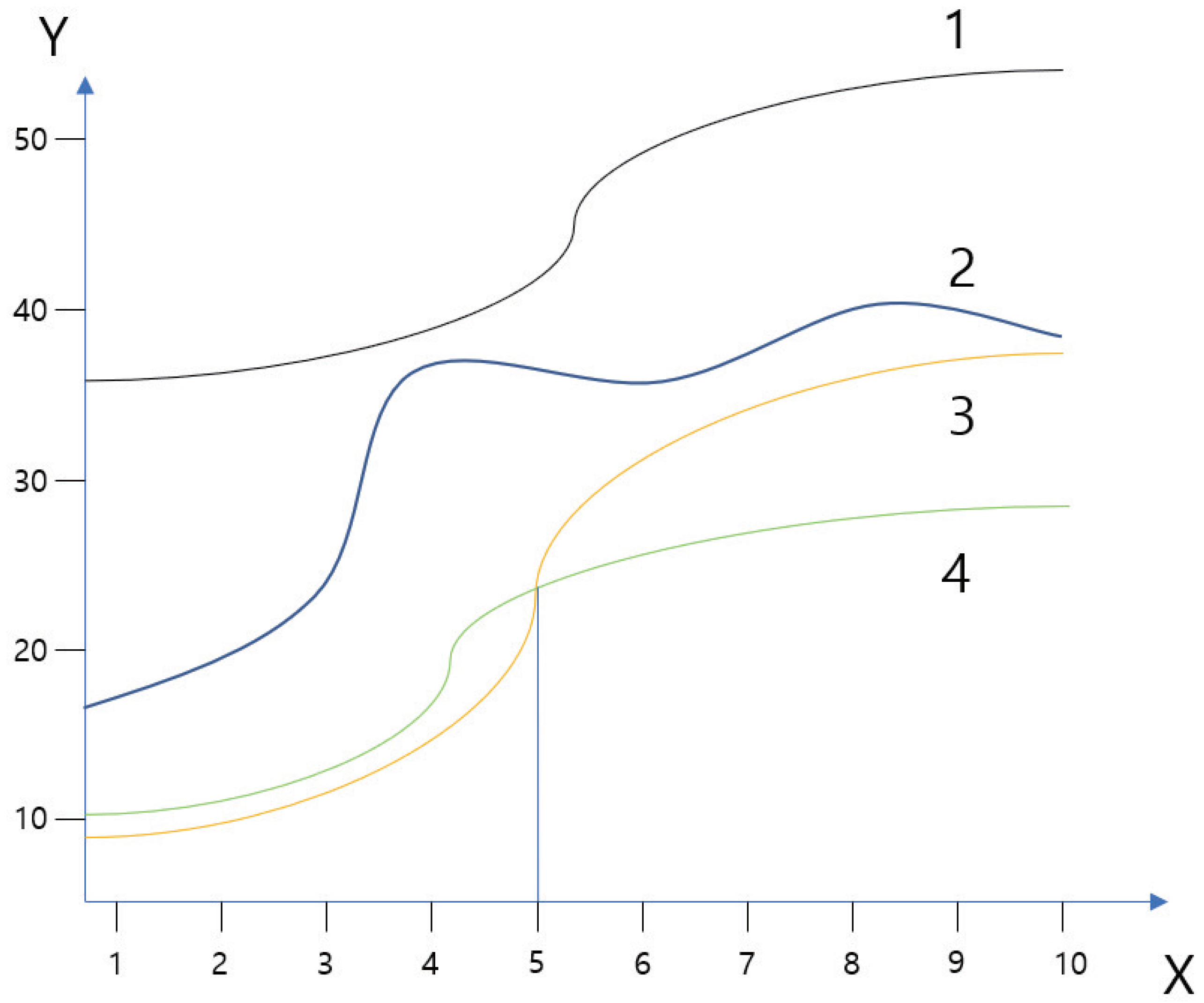
3. Methods
4. Experiments
4.1. Data
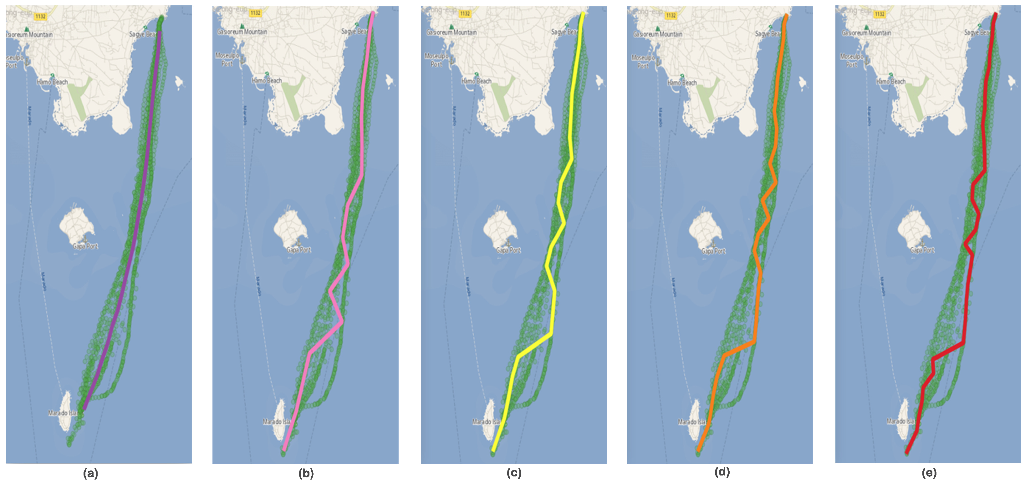
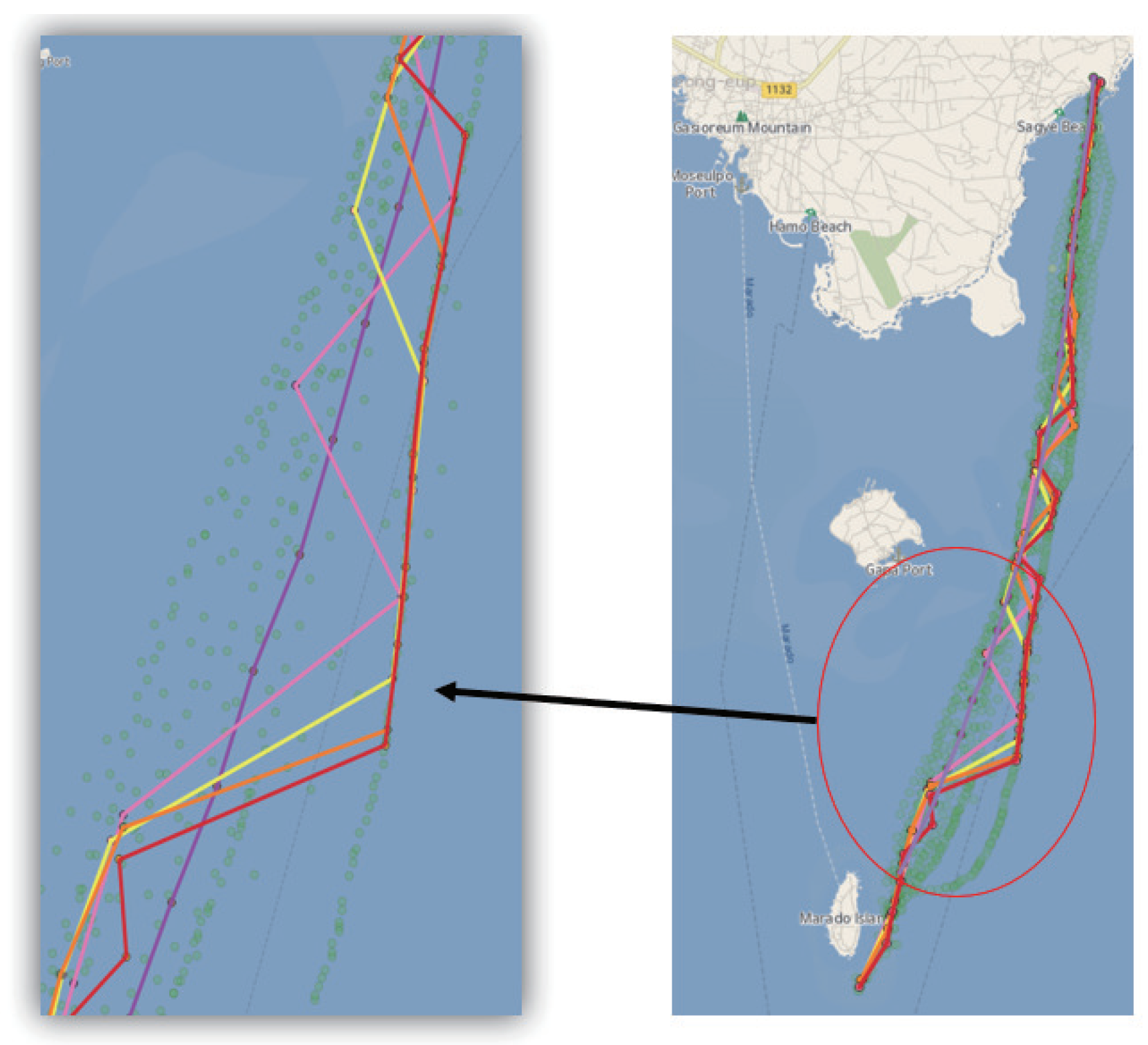
4.2. Case 1: Jeju Island Unjin Port to Mara Island Saledok Port
4.3. Case 2: Jeju Island Sagye Port to Mara Island Saledok Port
5. Discussion and Conclusions
Author Contributions
Funding
Conflicts of Interest
References
- Ahmed, M.; Karagiorgou, S.; Pfoser, D.; Wenk, C. Map construction algorithms. In Map Construction Algorithms; Springer: Berlin, Germany, 2015; pp. 1–14. [Google Scholar]
- Haklay, M.; Weber, P. Openstreetmap: User-generated street maps. IEEE Pervasive Comput. 2008, 7, 12–18. [Google Scholar] [CrossRef]
- Agamennoni, G.; Nieto, J.I.; Nebot, E.M. Robust inference of principal road paths for intelligent transportation systems. IEEE Trans. Intell. Transp. Syst. 2010, 12, 298–308. [Google Scholar] [CrossRef]
- Ahmed, M.; Wenk, C. Constructing street networks from GPS trajectories. In European Symposium on Algorithms; Springer: Berlin, Germany, 2012; pp. 60–71. [Google Scholar]
- Biagioni, J.; Eriksson, J. Inferring road maps from global positioning system traces: Survey and comparative evaluation. Transp. Res. Rec. 2012, 2291, 61–71. [Google Scholar] [CrossRef]
- Jeong, M.H.; Lee, D.H.; Lee, T.Y.; Lee, J.H. Robust local spatial autocorrelation analysis of massive vessel movements. J. Coast. Res. 2019, 91, 306–310. [Google Scholar] [CrossRef]
- Ramsay, J.O. Functional data analysis. Encycl. Stat. Sci. 2004, 4. [Google Scholar] [CrossRef]
- Duran, D.; Sacristán, V.; Silveira, R.I. Map construction algorithms: An evaluation through hiking data. In Proceedings of the 5th ACM SIGSPATIAL International Workshop on Mobile Geographic Information Systems, Burlingame, CA, USA, 31 October 2016; pp. 74–83. [Google Scholar]
- Edelkamp, S.; Schrödl, S. Route planning and map inference with global positioning traces. In Computer Science in Perspective; Springer: Berlin, Germany, 2003; pp. 128–151. [Google Scholar]
- Davies, J.J.; Beresford, A.R.; Hopper, A. Scalable, distributed, real-time map generation. IEEE Pervasive Comput. 2006, 5, 47–54. [Google Scholar] [CrossRef]
- Quddus, M.A.; Ochieng, W.Y.; Noland, R.B. Current map-matching algorithms for transport applications: State-of-the art and future research directions. Transp. Res. Part E Merg. Technol. 2007, 15, 312–328. [Google Scholar] [CrossRef]
- Cao, L.; Krumm, J. From GPS traces to a routable road map. In Proceedings of the 17th ACM SIGSPATIAL international conference on advances in geographic information systems, Seattle, WA, USA, 3–6 November 2009; pp. 3–12. [Google Scholar]
- Karagiorgou, S.; Pfoser, D. On vehicle tracking data-based road network generation. In Proceedings of the 20th ACM SIGSPATIAL International Conference on Advances in Geographic Information Systems, Redondo Beach, CA, USA, 6–9 November 2012; pp. 89–98. [Google Scholar]
- Wilcox, R.R. Introduction to Robust Estimation and Hypothesis Testing, 4th ed.; Academic Press: Cambridge, MA, USA, 2016. [Google Scholar]
- Sun, Y.; Genton, M.G. Functional boxplots. J. Comput. Graph. Stat. 2011, 20, 316–334. [Google Scholar] [CrossRef]
- López-Pintado, S.; Jornsten, R. Functional analysis via extensions of the band depth. In Lecture Notes—Monograph Series; Institute of Mathematical Statistics: Shaker Heights, OH, USA, 2007; pp. 103–120. [Google Scholar]
- Jeong, M.H.; Cai, Y.; Sullivan, C.J.; Wang, S. Data depth based clustering analysis. In Proceedings of the 24th ACM SIGSPATIAL International Conference on Advances in Geographic Information Systems, New York, NY, USA, 31 October–3 November 2016; p. 29. [Google Scholar]
- Jeong, M.H.; Sullivan, C.J.; Gao, Y.; Wang, S. Robust abnormality detection methods for spatial search of radioactive materials. Trans. GIS 2019, 23, 860–877. [Google Scholar] [CrossRef]
- Zuo, Y.; Serfling, R. General notions of statistical depth functions. Ann. Stat. 2000, 28, 461–482. [Google Scholar] [CrossRef]
- Serfling, R. Depth functions in nonparametric multivariate inference. DIMACS Ser. Discret. Math. Theor. Comput. Sci. 2006, 72, 1. [Google Scholar]
- Mosler, K. Robustness and Complex Data Structures. In Robustness and Complex Data Structures: Festschrift in Honour of Ursula Gather; Chapter Depth Statistics; Becker, C., Fried, R., Kuhnt, S., Eds.; Springer: Berlin, Germany, 2013; pp. 17–34. [Google Scholar]
- López-Pintado, S.; Romo, J. On the concept of depth for functional data. J. Am. Stat. Assoc. 2009, 104, 718–734. [Google Scholar] [CrossRef]
- Ramsay, J.O.; Wickham, H.; Graves, S.; Hooker, G. FDA: Functional Data Analysis. 2018. R Package Version 2.4.8. Available online: https://cran.r-project.org/web/packages/fda/fda.pdf (accessed on 28 January 2020).
- Varmuza, K.; Filzmoser, P. Introduction to Multivariate Statistical Analysis in Chemometrics; CRC Press: Boca Raton, FL, USA, 2016. [Google Scholar]


© 2020 by the authors. Licensee MDPI, Basel, Switzerland. This article is an open access article distributed under the terms and conditions of the Creative Commons Attribution (CC BY) license (http://creativecommons.org/licenses/by/4.0/).
Share and Cite
Jeong, M.-H.; Jeon, S.-B.; Lee, T.-Y.; Youm, M.K.; Lee, D.-H. Vessel Trajectory Reconstruction Based on Functional Data Analysis Using Automatic Identification System Data. Appl. Sci. 2020, 10, 881. https://doi.org/10.3390/app10030881
Jeong M-H, Jeon S-B, Lee T-Y, Youm MK, Lee D-H. Vessel Trajectory Reconstruction Based on Functional Data Analysis Using Automatic Identification System Data. Applied Sciences. 2020; 10(3):881. https://doi.org/10.3390/app10030881
Chicago/Turabian StyleJeong, Myeong-Hun, Seung-Bae Jeon, Tae-Young Lee, Min Kyo Youm, and Dong-Ha Lee. 2020. "Vessel Trajectory Reconstruction Based on Functional Data Analysis Using Automatic Identification System Data" Applied Sciences 10, no. 3: 881. https://doi.org/10.3390/app10030881
APA StyleJeong, M.-H., Jeon, S.-B., Lee, T.-Y., Youm, M. K., & Lee, D.-H. (2020). Vessel Trajectory Reconstruction Based on Functional Data Analysis Using Automatic Identification System Data. Applied Sciences, 10(3), 881. https://doi.org/10.3390/app10030881