Article

Regularization-Based Dual Adaptive Kalman Filter for Identification of Sudden Structural Damage Using Sparse Measurements

1
Korea Institute of Civil Engineering and Building Technology, Ilsan 10223, Korea
2
Department of Civil and Environmental Engineering, Seoul National University, Seoul 08826, Korea
*
Author to whom correspondence should be addressed.
Appl. Sci. 2020, 10(3), 850; https://doi.org/10.3390/app10030850
Submission received: 30 December 2019 / Revised: 16 January 2020 / Accepted: 20 January 2020 / Published: 25 January 2020
(This article belongs to the Special Issue Vibration-Based Structural Health Monitoring)

Abstract

:

Featured Application

The dual adaptive filter proposed in this paper can identify sudden change in structural systems under dynamic excitations. The proposed filter method including the tuning process can be applied to a variety of engineering areas in which near-real-time tracking of system parameter is needed.

Abstract

This paper proposes a dual adaptive Kalman filter to identify parameters of a dynamic system that may experience sudden damage by a dynamic excitation such as earthquake ground motion. While various filter techniques have been utilized to estimate system’s states, parameters, input (force), or their combinations, the filter proposed in this paper focuses on tracking parameters that may change suddenly using sparse measurements. First, an advanced state-space model of parameter estimation employing a regularization technique is developed to overcome the lack of information in sparse measurements. To avoid inaccurate or biased estimation by conventional filters that use covariance matrices representing time-invariant artificial noises, this paper proposes a dual adaptive filtering, whose slave filter corrects the covariance of the artificial measurement noises in the master filter at every time-step. Since it is generally impossible to tune the proposed dual filter due to sensitivity with respect to parameters selected to describe artificial noises, particle swarm optimization (PSO) is adopted to facilitate optimal performance. Numerical investigations confirm the validity of the proposed method through comparison with other filters and emphasize the need for a thorough tuning process.

1. Introduction

In various engineering fields, identifying the uncertain status of structural systems is a critical task to avoid severe malfunctions due to degradation of system parameters caused by deterioration or sudden damage by natural or man-made disasters. Among various approaches to such system identification (SI), there have been notable research efforts for probabilistic SI to handle uncertainties in the problem. For instance, Tarantola (1987) formulated SI as a Bayesian inverse problem, in which a joint probability density function (PDF) was introduced for parameters of systems under static loads [1]. Gaussian assumption was used for both prior and posterior distributions. Recently, such approach was extended by several probabilistic SI methods utilizing Bayesian Network, Markov Chain Monte Carlo, and Branch-and-Bound method [2,3,4,5,6]. Although these methods can handle general distribution models for prior and posterior, they are still subject to fundamental limitations for dynamic systems, i.e., systems under dynamic loads.
For precise updates of knowledge of a dynamic system based on the given measurements, sequential Bayesian filters including Kalman filter have been utilized [7,8,9,10]. The main strength of Bayesian filters comes from their two complementary updates: time-update and measurement-update. In this approach, by employing models that are respectively describing time- and measurement-updates using common random variables, a given dynamic system does not need to be expressed as one highly complicated joint PDF. To apply a filter method to dynamic system identification, it is vital to build an accurate state-space model that represents the dynamic system by two numerical models respectively describing the time- and measurement-updates. Then, a suitable filter method should be selected especially when the state-space model is nonlinear or time-variant.
To track the status of nonlinear dynamic systems, the extended Kalman filter (EKF) has been utilized [7,11]. EKF uses first-order linearization to approximate underlying statistics of the state-space model, but this filter may suffer from some limitations including the requirement of sufficient differentiability of the dynamic model. To overcome this inherent problem, the unscented Kalman filter (UKF) was developed using so-called unscented transformation [10,12]. This transformation linearizes nonlinear dynamic model by using “sigma points” instead of the derivatives. Using the UKF as the basic filter method, this paper develops a near-real-time SI method for dynamic systems that may experience time-varying changes in system parameters caused by damage. To handle this target problem with sparsely measured accelerations, the state-space model of this study, which is generally used in parameter estimation only [13], utilizes the Newmark model to update modal-displacement, velocity, and acceleration with current system parameters for just one time-update. Then, regularization techniques with an assumed prior information about system are introduced to the state-space model to avoid divergence in estimations caused by sparse measurements.
Even if a proper state-space model is constructed for time-varying systems, conventional filters such as EKF and UKF using time-invariant artificial noises may not be able to achieve accurate estimations. This is because the covariance matrices of artificial noises, which are arbitrarily chosen to satisfy the optimality condition of filter during a certain time interval, may not be optimal as the statistical characteristics of measurements change over the excitation period. To address this issue, the UKF should be able to determine new artificial noises at every time step to satisfy the optimality condition. The authors thus explored several adaptive filtering techniques, which can adapt to time-varying statistical characteristics of measurements [11,13,14,15,16,17]. Through these investigations, the dual adaptive filtering for artificial measurement noise estimation is finally selected and used along with the state-space model.
It is also noted that the dual adaptive filtering, which adopts a slave filter to update artificial-measurement-noise of the master filter, requires additional selection of artificial noise covariance matrices for the slave filter. The increased number of covariance matrices of artificial noises makes it challenging to tune dual adaptive filter for various choices of those covariance matrices. It is difficult to select proper artificial noises of slave filter empirically due to the absence of accurate knowledge [13,15,18]. Therefore, it is important to construct a general framework for tuning process of dual adaptive filtering. For this purpose, particle swam optimization (PSO), which was utilized in a recent study to tune Kalman filter for mobile robot attitude estimation [14], is adopted for dual filtering with appropriate assumptions to decrease the number of tuning parameters. However, this tuning process should be performed thoroughly because of randomness in the PSO algorithm. This study thus aims to improve estimation of dual filtering by performing PSO again with different boundary conditions. In numerical investigations, the estimation results by the proposed approach will be presented along with several considerations including the use of iterative tuning process.
This paper first introduces the algorithm of UKF with its general formulation for dynamic state-space model in Section 2. Various applications of filter methods will be also mentioned together with practical issues. Then, Section 3 introduces the problem statement of dynamic system, which can be damaged during seismic excitations. A proper state-space model is proposed and explored to choose appropriate adaptive filtering techniques. In Section 4, for an actual earthquake excitation, several damage scenarios are assumed based on the calculated time histories of relative displacement between adjacent stories. For these scenarios, accuracy and robustness of the proposed method are tested and demonstrated in comparisons with normal UKF and other adaptive filtering techniques. Lastly, this paper concludes with several insights and future research topics.

2. Background: Identification of Dynamic Systems by Unscented Kalman Filter

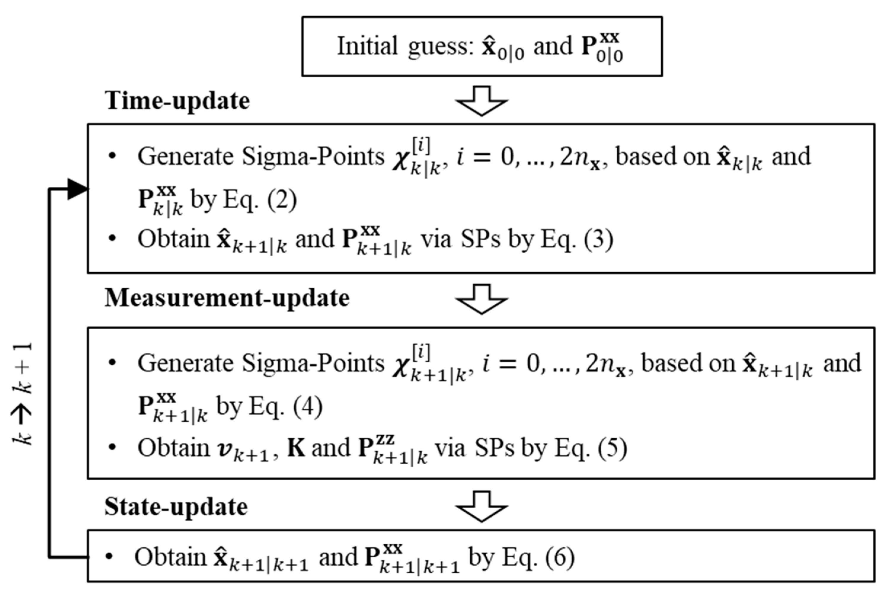
2.1. A Brief Review of Unscented Kalman Filter

To overcome the aforementioned challenges in using EKF for estimation of nonlinear state-space models, Julier and Uhlmann (2004) developed Unscented Kalman Filter (UKF) [12], also known as Sigma-Point Kalman Filter (SPKF). The unscented transformation of UKF is based on a statistical technique using sigma points (SPs), which provides derivative-free state estimation for a nonlinear state-space model. UKF is known to achieve the second-order accuracy with the same computational complexity as that of EKF.
For details of UKF, let us consider a dynamic state-space model governed by a set of discrete-time nonlinear equations [19]
x k + 1 = f ( x k ) + w k z k + 1 = h ( x k + 1 ,   u k + 1 ) + v k + 1
where k is the time index; x k R n x × 1 is the state vector representing displacement, velocity, or system parameters such as elasticity and damping coefficient at time t k ; f ( · ) and h ( · ) respectively denote nonlinear system-process model and measurement-output model; w k R n x × 1 represents the artificial process noise modeled by a Gaussian random vector with zero means and covariance matrix Q k R n x × n x , i.e., w k ~ N ( 0 , Q k ) ; z k R n z × 1 is the vector of the measured quantities such as acceleration; u k is the vector of inputs; and v k R n z × 1 denotes artificial measurement noise modelled as v k ~ N ( 0 , R k ) . The noises w k and v k are assumed to be uncorrelated with each other.
Figure 1 illustrates the general algorithm of UKF [20]. In the figure, x ^ k | k and P k | k x x respectively denote the mean (column) vector and covariance matrix of the states at the k-th time step ( k = 0 , 1 , ) before the updates are performed. At each time step, sigma points (SPs) χ k | k [ i ] , i = 0 , , 2 n x , are first generated based on x ^ k | k and P k | k x x as
χ k | k [ 0 ] = x ^ k | k χ k | k [ i ] = x ^ k | k + ( ( n X + κ ) P k | k x x ) i ,   i = 1 , , n X χ k | k [ i ] = x ^ k | k ( ( n X + κ ) P k | k x x ) i n X , i = n X + 1 , , 2 n X
where the square-root symbol denotes the “matrix square root”, which can be computed by Cholesky factorization [20], and (   ) i indicates the i-th column vector of the matrix. The tuning parameter κ is often used to consider high order moments in the approximation and assumed to be zero in this paper. Next, using the system-process model f ( ) , x ^ k | k and P k | k x x are updated to x ^ k + 1 | k and P k + 1 | k x x , respectively, via the sigma points in Equation (2). In detail, this “time-update” is performed as
χ k + 1 | k [ i ] = f ( χ k | k [ i ] )   x ^ k + 1 | k = i = 0 2 n X W m i χ k + 1 | k [ i ]   P k + 1 | k x x = i = 0 2 n X W c i [ χ k + 1 | k [ i ] x ^ k + 1 | k ] [ χ k + 1 | k [ i ] x ^ k + 1 | k ] T + Q k
where W m i and W C i are the weighting coefficients of SPs for which W m 0 = W C 0 = κ / ( n X + κ ) and W m i = W C i = 1 / 2 ( n X + κ ) are used [19]. x ^ k + 1 | k and P k + 1 | k x x in Equation (3) are considered prior estimates of the states at the k-th time step.
For the “measurement-update” of the prior estimates in Figure 1, SPs are first generated as
χ k + 1 | k [ 0 ] = x ^ k + 1 | k χ k + 1 | k [ i ] = x ^ k + 1 | k + ( P k + 1 | k x x ) i ,   i = 1 , , n X χ k + 1 | k [ i ] = x ^ k + 1 | k ( P k + 1 | k x x ) i n X , i = n X + 1 , , 2 n X
Then, the measurement-updates are performed to obtain the following sequentially:
ζ k + 1 | k [ i ] = h ( χ k + 1 | k [ i ] ) ,   i = 0 , , 2 n X z ^ k + 1 | k = i = 0 2 n X W m i ζ k + 1 | k [ i ] v k + 1 = z k + 1 z ^ k + 1 | k P k + 1 | k z z = i = 0 2 n X W C i [ ζ k + 1 | k [ i ] z ^ k + 1 | k ] [ ζ k + 1 | k [ i ] z ^ k + 1 | k ] T + R k + 1 P k + 1 | k x z = i = 0 2 n X W C i [ χ k + 1 | k [ i ] x ^ k + 1 | k ] [ ζ k + 1 | k [ i ] z ^ k + 1 | k ] T K = P k + 1 | k x z ( P k + 1 | k z z ) 1
where ζ k + 1 | k [ i ] is an SP calculated by substituting χ k + 1 | k [ i ] to the function h ( · ) ; v k is an innovation vector, i.e., theoretical residuals; P k + 1 | k z z and P k + 1 | k x z are covariance of the measurements and cross covariance of state and measurements; and K is the calculated Kalman gain.
Finally, the results of the two updates are used to obtain the posterior estimates of the states and covariance matrix by the “state-update” step, i.e.,
x ^ k + 1 | k + 1 = x ^ k + 1 | k + K v k + 1 P k + 1 | k + 1 x x = P k + 1 | k x x K P k + 1 | k z z K T
These time-, measurement- and state-updates are performed at each time step k using the results of the previous step as illustrated in Figure 1.

2.2. Applications of Filter Methods and Practical Issues

In applications of filter methods to structural systems, it is generally assumed that the accelerations can be measured. For the purpose of state estimation, parameter estimation, or input estimation, the corresponding state vector is respectively defined in terms of the dynamic responses (e.g., displacement and velocity), system parameters (e.g., Young’s modulus, damping coefficient, and parameters of Bouc-Wen hysteretic models), or input forces. If system parameters are estimated concurrently with dynamic responses, the filter is termed as joint state-parameter estimation. In the so-called joint input-state estimation, input forces are estimated together with the responses.
For example, as a joint state-parameter estimation, Yang et al. (2006) proposed an adaptive EKF-based tracking technique to detect sudden damage in a five-story linear structure [11]. Wu and Smyth (2007) applied UKF to a nonlinear system having 2 degrees of freedom (DOFs) for the purpose of SI to find that the UKF provided better estimation than EKF for highly nonlinear systems [21]. Chatzi and Smyth (2009) also utilized UKF for SI of nonlinear 3-DOF structural system assuming non-collocated heterogeneous sensing [22]. Most previous studies on joint state-parameter estimation have focused on improving performance of filters in tracking parameters of highly nonlinear structural system. These studies employed the system equation of motion under the assumption that either acceleration or displacement is measured at every DOF to avoid rank-deficiency. However, measuring dynamic responses at all DOFs is infeasible especially for structures consisting of many components. This may limit the applicability of joint state-parameter estimation to SI in practice.
Recently, many research efforts have been made regarding the joint input-state estimation to track the input force whose exact information is not available in many situations. Gillijns and De Moor (2007) proposed the recursive-three-step filter (RTSF), which updates responses and input force at the different step, for unbiased minimum-variance estimation of input and state [23]. Since RTSF suffered from rank-deficiency caused by a limited number of measured acceleration or reduced-order model from modal analysis, Lourens et al. (2012) proposed an advanced version of RTSF by using truncated covariance matrices through singular value decomposition [24]. Azam et al. (2015) developed a dual Kalman filter consisting of two stages to prevent numerical issues such as un-observability and rank-deficiency of RTSF when using sparse acceleration measurements [25]. Aucejo et al. (2019) proposed an augmented Kalman filter, whose state vector consists of responses and input together, with the state-space model developed based on the generalized-α method [18]. This was to address the issue that the dual Kalman filter is sensitive to selection of covariance matrices of artificial noises. These studies focused on joint input-state estimation of linear structural systems with time-invariant system parameters. Although full-measurements are not required because of the linear model assumption, rank-deficiency and divergence are still critical issues when SI relies on sparse measurements or a reduced-order model is used.
Meanwhile, as a parameter estimation example, Astroza et al. (2019) applied UKF to Finite-Element (FE) updating with adaptive techniques to consider uncertainty of nonlinear FE models [13]. The state-space model based on Newmark method was able to utilize sparse measurements whereas the use of equilibrium equations in state-space models of previous joint state-parameter estimations needs full measurements. Then, dual adaptive filtering was performed based on the proposed state-space model to consider uncertainty in FE model. The applications using three different approaches, i.e., joint state-parameter estimation, input-state estimation, and parameter estimation confirmed that the state-space model must be developed appropriately based on target estimations, and it is essential to use a proper filtering method to obtain optimal estimations.
It is also noted that, in all filter-related research, it is critical to tune the filter by selecting covariance matrices Q k and R k which describe uncertainties of the artificial noises in system-process and measurement-output model respectively. Although the tuning process of those covariance matrices is vital for good filter performance, there is no general technique available. In efforts to handle this, many studies assumed that the artificial measurement noise can be prescribed using the available specifications of the sensors. Then, the artificial process noise is determined by minimizing the root mean square (RMS) of time-history “innovations,” which are defined as follows, to quantify the differences between measurements and responses corresponding to the system parameters predicted during the time-update part [13,16]:
f I ( Q k ) = 1 n T ( k = 0 T v k ( Q k ) 2 )  
where v k ( Q k ) is an innovation vector defined for the time duration k = 0 , , T ; and n T = T + 1 . In several references [25,26], it has been shown that f I ( Q k ) in Equation (7) tends to decrease following an L-shaped curve as Q k increases. Generally, the inflection point of the L-shaped curve is recommended as a near-optimal solution in terms of the filter performance. The opposite case, in which the artificial process noise is known, and the corresponding artificial measurement noise is to be determined, can be solved in a similar manner. If both types of artificial noises are unknown, the objective function can feature both Q k and R k . To address this, for instance, Odry et al. (2018) utilized particle swarm optimization (PSO) [14]. In this paper, PSO is used to obtain the best tuning parameters of the proposed dual adaptive filtering.

3. Proposed Method: Adaptive Unscented Kalman Filter Using Sparse Measurements of Accelerations

3.1. Regularization-Based State-Space Model

This paper aims to develop a near-real-time system identification method for structures under disastrous dynamic loads such as earthquake excitations. In particular, the method focuses on detecting sudden changes in the system parameters such as Young’s modulus caused by structural damage during excitations. It is assumed that input data such as an earthquake (EQ) ground motion has been acquired accurately. Conventional filter methods such as EKF and UKF show limitations in tracking the status-history having discontinuity points because those methods using constant artificial noises cannot adapt to time-varying statistics in the measurements. To address this issue, Yang et al. (2006) proposed an adaptive joint state-parameter estimation method requiring full measurement condition, which is however not available in general practice [11]. The adaptive rule was tested with simple events where just one component experiences sudden damage. On the other hand, state-space models in joint input-state estimations do not accord with the objective of this paper because those models are constructed based on modal analysis for which the system parameters are assumed to be time-invariant.
To facilitate SI under practical measurement conditions, we aim to develop a filter that performs well even with sparse measurements. To this end, let us first consider the following state-space model proposed by Astroza et al. (2019) for the purpose of parameter estimation [13]:
x k + 1 = x k + w k
z k + 1 = h ( x k + 1 ,   u 0 ,   u ˙ 0 ,   p 1 : k + 1 ) + v k + 1
where x k is the state vector representing parameters to estimate, e.g., Young’s moduli at time t k ; u 0 and u ˙ 0 are the initial displacement and velocity respectively (hereafter, the dot means time-derivative); and p 1 : k + 1 denotes the time-history of excitation up to t k + 1 , e.g., seismic loads. The function h ( · ) represents a response function from an FE model, e.g., the Newmark method ( γ = 1 / 2 ,   β = 1 / 4 ). The system-process model in Equation (8) is linear, thus Equation (3) can be simplified into x ^ k + 1 | k = f ( x ^ k | k ) and P k + 1 | k x x = P k | k x x + Q k in this case, i.e., without deriving SPs as in Equation (2). The measurement-output model in Equation (9) predicts responses, which will be compared with the measured response. In this state-space model, full-measurement is not required because the measurement-output model adopts the response function rather than the equilibrium equation.
It is noted that the measurement-output model in Equation (9) was originally designed for time-invariant system parameters. Consequently, a transient period can appear as the estimations of conventional filter converge into the changed status of damaged components. If that transient period is considerably long, it may hamper accurate estimations. To address this limitation of the state-space model of Equations (8) and (9) in SI of time-variant systems, Equation (9) is modified as follows to track sudden changes:
q ˜ k + 1 = h ( x k + 1 ,   q ˜ k ,     p k + 1 )
z k + 1 = S Φ ( x k + 1 ) q ˜ k + 1 T + v k + 1
where q ˜ k is the matrix consisting of modal displacement, velocity, and acceleration, i.e., q ˜ k = [ q k   q ˙ k   q ¨ k ] ; q ˜ 0 = Φ ( x 0 ) 1 [ u 0   u ˙ 0   u ¨ 0 ] ; Φ R n DOF × n DOF is the matrix of the mode shapes consisting of the eigenvectors Φ j , j = 1 , , n D O F (calculated from undamped eigenvalue problem K Φ = M Φ Ω 2 , where K , M , and Ω are stiffness, dumped mass matrix, and a diagonal matrix of the eigen frequencies, respectively); and S n DOF × 3 is the selection matrix for the measured responses. In Equation (9), at every time step, the current response such as acceleration is calculated from initial responses, which becomes a computational burden as the amount of calculation increases linearly as time goes on. By contrast, Equation (10) uses the Newmark method to predict the next modal responses based on the current information, i.e., system parameters estimated from time-update part and modal responses of the previous time-step. This modified measurement-output model facilitates handling time-variant system parameters. In Equation (11), the vector of the predicted modal responses is transformed to nodal responses by the matrix of calculated mode shapes. Each element in the selection matrix is set as 1 if measurements are made at the corresponding DOF. Finally, the nodal responses predicted by the changed system parameters are matched to the measured responses to calculate the Kalman gain.
The state-space model consisting of Equations (8), (10) and (11) may achieve desirable accuracy of estimation in some cases. However, when using sparse measurements, it has been reported that even if the predicted response well matches the measured responses, unobserved response quantities may be considerably different from the actual ones due to the biased estimation of parameters [27]. Noise in sparse measurement may exacerbate the bias and instability of estimation. To alleviate this undesirable situation, this paper proposes to utilize a regularization technique to avoid rapid and wrong transitions during the estimation. In particular, adopting a well-known regularization technique, Tikhonov term is included in the objective function with a regularization factor to obtain stabilized solutions based on a priori information and the measurements [28,29,30,31,32]. From the Bayesian perspective, the Tikhonov term corresponds to a prior (as a normal distribution in general) to inform a possible solution space [1]. In detail, a regularization term is added to measurement-output model as constraints as follows:
x k + 1 = x ^ P + r x where   x ^ P = i = k N w k x ^ i
where x ^ P is a vector representing prior information about system parameters, which is updated at every time-step in Equation (12); r x denotes the standard deviation of prior as regularization factor to constrain the estimation, i.e., x k ~ N ( x ^ P ,   Σ ) and d i a g ( Σ ) = r x 2 ; and N w is set up as 5% of n T . Actually, it is a critical issue to determine the regularization factor in existing studies of regularization. In this paper, the regularization factor in Equation (12) is selected intuitively not to increase the number of tuning parameters. Because the following dual adaptive filtering techniques requires more than two tuning parameters, it is not desirable to further increase the number of those parameters. The assumption about intuitive selection will be explained in the part regarding numerical investigations.
By including the regularization term in the measurement-output model, stable estimation is achieved while avoiding divergence due to noisy sparse measurements. Therefore, this regularization-based state-space model is utilized in this study to track sudden damage in system parameters under seismic loads.

3.2. Dual Adaptive Filtering for Measurement Noise Estimation

For accurate estimation of time-variant system parameters, the advanced state-space model needs to be used in conjunction with a proper adaptive filtering technique. There are two reasons for the limited tracking ability of conventional filters when statistics in measurements change. First, the predicted state vector in the time-update part is influenced by the size of covariance of artificial process noise. Second, both covariance matrices of artificial process and measurement noises affect the calculation of the Kalman gain. Therefore, if both covariance matrices are constant during estimation, the tracking performance of conventional filters will be limited for time-variant dynamic system.
While developing the proposed filter, a few other adaptive techniques were explored. For example, Liu et al. (2005) proposed an adaptive tracking technique for the purpose of leak detection and location in the management of a pipeline system [17]. This tracking technique was performed based on particle filter, which is also known as a sequential Monte Carlo method. However, it is noted that the idea of adaptive technique is utilized also in the UKF-based approaches. The details and limitations of this technique (with modification for UKF) are described in Appendix A. It is especially noted that this adaptive technique controls the artificial process noise, which causes severe bias and instability of estimations. The other adaptive technique explored in this study is a master-slave Kalman filter (MS-KF), which is also called as a dual adaptive filtering. The main concept of MS-KF is that, when a master filter (MF) estimates the given random variables, the slave filter (SF) will estimate the covariance matrix of either artificial process or measurement noises in MF at every time-step. There are two types of MS-KF based on process noise estimation (MS-KFPE) and measurement noise estimation (MS-KFME). Among these, details of MS-KFPE are briefly presented in Appendix B because MS-KFPE is not suitable for the goal of this study for the same reason as the adaptive technique described in Appendix A.
Unlike the two techniques mentioned above, MS-KFME controls artificial measurements noise and can be utilized with the advanced state-space model. The general algorithm of MS-KF is illustrated by a block diagram in Figure 2. In the slave filter (SF) part, two random variables ω k R n x × 1 and υ k R n z × 1 represent the artificial noises for process and measurements respectively modeled as ω k ~ N ( 0 , T ) and υ k ~ N ( 0 , U ) in which T R n x × n x and U R n z × n z are time-invariant covariance matrices; and the superscript S indicates a variable related to the SF. A well-known drawback of MS-KF is its sensitivity with respect to the choice of two covariance matrices of artificial noises in SF. Therefore, these artificial noises should be selected carefully with those of MF [15,27]. Linear KF (LKF) is utilized for SF in most cases because there is no accurate knowledge available for the state-space model [15]. In this paper, a covariance-matching technique is utilized in the state-space model of SF because this intuitive technique can be implemented easily with low computational costs [13,15,27,33].
In Figure 2, using the equations related to the number (2) indicates that the MS-KF estimates the covariance of artificial measurements noise at every time-step of MF [13,15] (if the equations noted by the number (1) are used, MS-KFPE is performed). MS-KFME can be conducted based on two types: “the innovation and its covariance” or “the residual and its covariance”. In this paper, the latter one is selected because its calculations are less complex.
The goal of SF in MS-KFME is to make the innovations, which is employed to provide a measure of optimality of the filter, compatible with their expected covariance matrix. For this purpose, the covariance-matching technique is conducted, i.e.,
z k + 1 s = d i a g ( E [ v k + 1 v k + 1 T ] )
I k + 1 = d i a g ( i = 0 2 n x W c i [ ζ k + 1 | k i z ^ k + 1 | k ] [ ζ k + 1 | k i z ^ k + 1 | k ] T )
where Equation (13) represents the actual covariance based on innovations, and the Equation (14) is the predicted covariance of innovations from MF. If two matrices from Equation (13) and (14) are similar to each other, the current covariance of artificial measurement noise of MF is considered appropriate. If the calculated value of Equation (13) is larger than that of Equation (14), R k + 1 needs to be increased to avoid divergence of MF, and consequently this procedure increases the covariance of states, P k + 1 x x .
There are three advantages in using MS-KFME: First, no additional parameter is introduced for the algorithm (as for MS-KFPE, the time-window is required). Second, while the other two adaptive techniques shift the solution space rapidly by increasing Q k , MS-KFME widens the solution space by increasing P k + 1 x x . Indeed, the biased estimation may be avoided by increasing P k + 1 x x instead of increasing the size of Q k rapidly, and stable estimation will be achieved. Lastly, this correction process for artificial measurements noise is implemented in measurement-update of MF before calculating the Kalman gain. Therefore, the corrected covariance of artificial measurements noise by SF can be utilized immediately. These advantages enable MS-KFME to track the sudden decrease of system parameter in a stable manner during the seismic excitations.
The algorithm of MS-KFME with the newly proposed state-space model is summarized in Figure 3. In the time-update part, calculations of SPs are not needed because of the linear system-process model in Equation (8). The part corresponding to the slave LKF is represented in gray background along with detailed descriptions. It is noteworthy that the regularization term in Equation (12) is considered in the form of dummy variables [34] when the auto- and cross- covariance matrices are calculated in the measurement-update part of MF. In these calculations for two covariance matrices, the prior information of regularization is required. When the time-step is shorter than the selected time-window, the values of initial state are used for this prior information. After that time point, this prior is updated in the state-update part.

4. Numerical Investigations

4.1. SI under Simulated Damage Scenarios

To test the combination of the selected dual adaptive filtering techniques and the proposed state-space model based on regularization, a shear building having 6 DOFs in Figure 4 is investigated. The lumped mass of each floor is assumed as 1 kg, and Young’s modulus of all inter-story is equal to 1 Pa (i.e., inter-story stiffness of each floor is 24 N/m). Rayleigh damping, which is proportional to mass and stiffness matrices, is utilized by assuming a damping ratio of 5% for the first and second modes. For the linear system, Young’s modulus of each component is estimated using an EQ ground motion. The time-history of the 180-degree component of ground acceleration recorded at El Centro station during the earthquake event in 1940 with Mw = 6.95 is used in this numerical investigation. The length of this ground acceleration history is 42 s, and discretized by 0.01 s. To consider potential damage scenarios, the EQ time-history is first applied to the shear building without damage events. The relative displacements between adjacent stories are calculated to find the peak values at each story and the occurrence-time as shown in Table 1.
Based on the simulated sequence of peak displacements, five damage scenarios are created in terms of sudden decrease of Young’s moduli as summarized in Table 2. Scenarios 1 and 2 depict sequence of sudden decreases of story stiffness. Scenario 3 simulates a sequential failure initiated by the maximum-peak response at 5th story. Scenarios 4 and 5 are assumed to depict more complicated sequential scenarios. In Scenario 4, the second story experiences the additional sudden decrease 7.42 s after the initial decrease of corresponding story’s stiffness. Scenario 5 consists of three sudden decreases of different stories. After simulating the above scenarios, the condition of sparse measurements is defined such that accelerations at the first, second, fourth, and sixth story can be measured. From this assumption, the selection matrix S will be set up as S 13 = S 23 = S 43 = S 63 = 1 and S i j = 0 otherwise. Then, the noise-history, which is simulated from a uniform distribution between 95% and 105% of RMS of measured accelerations, is added to simulate noise in the measurements.

4.2. Tuning Process Using Particle Swarm Optimization

As stated in Section 2.2, all filter methods should be tuned by selecting proper covariance matrices of artificial noises to achieve an optimal estimation. In using LKF, EKF, and UKF, just one parameter is tuned. Although each diagonal term of those covariance matrices may require individual tunings, it is assumed that all elements in vectors of states and measurements have same statistical characteristics for simplicity. Generally, the covariance of artificial measurements noise is determined based on sensor specification. The last tuning parameter is then the covariance of artificial process noise and can be selected from the derived L-curve. However, this process does not work for adaptive filtering techniques, because more than two tuning parameters are required even under the assumption that sensor specification can determine the covariance of the artificial measurement noise. The tuning process for MS-KFME with the proposed state-space model handles three parameters, i.e., two parameters corresponding to covariance matrices of master and slave filters’ artificial process noise, and the regularization factor in the proposed state-space model. In this case, it is impossible to derive the L-curve for two tuning parameters.
This paper utilizes the particle swarm optimization (PSO) to tune the dual adaptive technique with the proposed state-space model. PSO was originally inspired by the information circulation and social behavior observed in bird flocks and fish schools and is suited to solve problems where the optimal solution is a point in a multi-dimensional space of the parameter [35]. Odry et al. (2018) showed that PSO can find proper tuning parameters for optimal estimation performance [14]. However, if there are many variables in global optimization problem, this optimization process may give a computational burden. This is because PSO uses many particles to probe the best in the solution space, and the required number of particles increases exponentially as the number of tuning parameters increases. Another issue is that the performance of MS-KF is sensitive to choices of covariance matrices of artificial noises for master and slave filter. Actually, the positive definiteness condition for calculating SPs related with Equations (2) and (4) may be violated by subtle changes in those covariance matrices, and this numerical issue will interrupt the procedure of UKF as master filter. Therefore, it is desirable to decrease the number of tuning parameters in PSO for stable tuning process, and thus, the following assumptions will be introduced.
First, the regularization factor in the proposed state-space model is assumed as 10% of initial states, which means that the solution space will be constrained by the normal probability density, i.e., x ~ N ( x ^ P , Σ ) and d i a g ( Σ ) = ( 0.1 · | x 0 | ) 2 . The reason for adopting the regularization was to support sequential estimations of filter to avoid divergence caused by the lack of information due to sparse measurements. Therefore, there is no need to select the accurate regularization factor necessarily because the regularization term can confine solution space weakly. In the following numerical examples, moderate damage, which cannot be inspected visually, is assumed. Thus, in this paper, 10% of initial states’ values is used as the regularization factor, which gave rapid convergence to the exact value. Other values may be also appropriate, but too small values such as 1% of initial values are likely to result in long transient period before converging to an accurate solution. Second, each diagonal term of covariance of artificial measurements noise is assumed as 5% of the RMS of measurements for master filter. This assumption of artificial measurements noise can be improved by accurate information about actual sensor specification. Similarly, the covariance of artificial measurement noise for slave filter is determined as 1% of the identity matrix for simplicity.
Through the above assumptions, two tuning parameters that control the size of covariance matrices of artificial process noise for master and slave filter are used as variables for PSO. As in Equation (7), these two parameters affect the innovation in the following objective function:
f I ( x 1 , x 2 ) = 1 n T ( k = 0 T v k ( Q ( x 1 ) , T ( x 2 ) ) 2 )   where   Q = d i a g ( | x 0 | · 10 x 1 )   and   T = I n x × n x · 10 x 2
in which x 1 and x 2 are tuning parameters, and I n x × n x is an identity matrix. The objective function in Equation (15) is constructed to find an optimal estimation having the least RMS of innovation-history. This paper used the PSO algorithm in the global optimization toolbox of 2018b-version of MATLAB®.
When performing PSO, there are two important points to achieve efficiency: (1) setting boundary conditions in PSO for random variables and (2) determining the number of particles representing initial locations. The boundary conditions constrain the solution space, and thus a wrong setting may lead to finding no optimal solution. In some cases, the results of PSO are located near boundaries. In this situation, PSO should be re-performed, and it is recommended to shift the relevant variables’ boundary to include the corresponding end. On the other hand, to determine the number of particles properly, the generated particles should be scattered uniformly around the whole solution space. For example, one could discretize uniformly in the range of each variable such as [0.1, 0.2, 0.3, …, 0.9]. In this case, the total number of particles is assumed as 81 for 2-dimentional problem.
There may be more efficient alternatives than using these recommendations. However, it is essential to perform PSO iteratively to find a near-optimal solution because of intrinsic randomness in PSO. Table 3 presents results of PSO using 81 particles about the damage scenarios with the selected boundary conditions given as [lower bound, upper bound]. In Scenarios 3 and 4, PSO was re-performed because the results were located at one of the boundaries.
With the tuning parameters obtained by PSO, the MS-KFME is conducted for the scenarios. For normal-UKF (n-UKF) and adaptive tracking technique-based UKF (AUKF) in Appendix A, PSO using Equation (15) (with the variable x2 excluded) is performed to determine x1 as 3.23 and 3.88, respectively. MS-KFPE (in Appendix B) was not performed due to the difficulty in selecting the size of time-window. Figure 5a–c shows the estimation results by the proposed method, n-UKF and AUKF, respectively, under Scenario 1. From the results, it is confirmed that, while the results of n-UKF and AUKF show biased estimations, the MS-KFME derives accurate estimations about all parameters. Although divergence in n-UKF and AUKF was avoided by adopting the regularization term into state-space model, those filters still converged into wrong values. These results show that filter methods, which control artificial process noise, cannot adapt to measurements, whose statistics change due to damage.
Figure 6 reports estimation results by MS-KFME for Scenario 2. After a short range of unstable estimation at around 11 s, the estimation converges to accurate values without bias. When initial boundaries by PSO (Table 3) are used for Scenario 3 (Figure 7a), the estimation of the fifth story’s parameter, where acceleration-history is missing, shows divergence after around 38 s. The estimations of first and third stories’ parameters are inaccurate and biased as well. Figure 7b shows that, when the newly derived PSO’s result is used, the bias in estimation of fifth story’s parameter disappears, and the accuracy of first and third stories’ estimations is improved. From these results, it is noted that the tuning process using PSO should be performed iteratively for finding the near-optimal solution.
Next, more complicated sequential damage scenarios are considered to test stable tracking-capability of the proposed method. The PSO’s result for Scenario 4 (the second story experiences the additional sudden damage after the initial damage) was derived at one of the boundaries. Thus, PSO was re-performed to find new tuning parameters reported in Table 3. The estimations with the newly derived tuning parameters are presented in Figure 8. In this figure, the first story’s parameter is not assumed to be damaged. By the way, the range from around 10 to 25 s shows slightly biased estimation of the first story, and this bias is being severe before the estimation approaches to the exact value at around 35 s. This is probably because the corresponding acceleration for the damaged third story is not measured, and the damage occurred at adjacent stories. It may be a burden for slave filter to infer accurate information based on only innovations from master filter without structural knowledge. However, as mentioned in Section 3.2, the MS-KFME aims to obtain stable estimations from sparse measurements by searching solution space gradually rather than rapid tracking. The results confirm that the estimations about adjacent stories are distinguishable and converged to accurate values respectively after the transient period.
Finally, Scenario 5, which consists of three sudden damages in three different stories, are investigated as shown in Figure 9. When compared with Scenario 4, this scenario assumes that the damage occurs at separate stories, and corresponding accelerations of these stories are measured. In this case, faster convergence to accurate values is achieved.

4.3. Further Investigations Using Different Ground Motions

To test general applicability of the proposed method, another real EQ ground motion is applied to the same shear building in Figure 4. The time-history of the 65-degree component of ground acceleration from the 1971 San Fernando earthquake (Mw = 6.61 at the ‘2516 Via Tejon PV’ station) is used. The 56-second-long time history is discretized by 0.005 s. This EQ ground motion matches an assumption that damage happens at the middle of EQ time-history. That is, when calculating the relative displacements between adjacent stories, the peak values were located around the middle of EQ time-history. In Table 4, the scenarios based on the calculated peak values are presented. In the previous numerical tests, the n-UKF and AUKF showed early convergence before approaching accurate values. Scenarios in this section require that MS-KFME should not be converged too early during the filtering-process and adapt to time-varying statistics of the measurements. From this further investigation, it is proved that the proposed method enables us to estimate status of system parameters without early convergence.
To derive tuning parameters in Equation (15), PSO using 81 particles was performed with boundary conditions as x 1 [ 3 ,   5 ] and x 2 [ 5 ,   10 ] . These boundary conditions, which are different from those in Table 3, are obtained by performing PSO several times. This result proves that PSO requires boundary conditions appropriate for the given problem, and PSO-based tuning process should be re-performed iteratively to obtain proper boundary conditions.
The results in Figure 10, Figure 11, Figure 12 and Figure 13 confirm that MS-KFME with parameters tuned by PSO can accurately detect the sudden damage of systems despite sparse and noisy measurements. These also demonstrate that the proposed method helps avoid early convergence and enables us to track status of system accurately throughout the excitation period. In Figure 11 about Scenario 2’, it is noted that the time-history of the fifth story’s target parameter decreases along with the damaged parameter of the fourth story, but the estimation of the fifth story’s parameter returns back to the accurate value. It should be noted that the proposed method achieves this result even though the acceleration of the fifth story was missing. A similar observation is made in Scenario 3’ where the fifth story is damaged instead of the fourth story. The results of Scenario 3’ in Figure 12 show better separation between the estimations of fourth and fifth stories when compared with the results of Scenario 2’. This phenomenon indicates that when acceleration-history, whose statistics change due to the damage of corresponding parameter, is measured, estimations are less stable than the opposite case. In Figure 13, the estimations in the range after successive damage are more accurate than those in the range corresponding to initial damage.

5. Conclusions and Topics for Future Study

In this paper, a novel methodology was proposed to track sudden damage of structural system under dynamic excitations using sparse measurements. First, the state-space model often used for the purpose of parameter estimation was modified to handle time-variant system parameters. The regularization term was also introduced to avoid divergence of estimation caused by sparse noisy measurements. Second, the master-slave Kalman filter for measurement noise estimation (MS-KFME) was utilized to adapt to time-varying status of the target system. The unscented Kalman filter (UKF) as master filter estimates the status of target system parameters while a linear Kalman filter (LKF) as slave filter estimates the covariance of artificial measurement noise in UKF through a covariance-matching technique. Lastly, particle swarm optimization (PSO) was exploited to tune the artificial noises of MS-KFME with practical considerations. To test the proposed methodology, sets of structural response data were simulated for a shear-building system subjected to two real earthquake ground motion time histories. Several damage scenarios were introduced based on the simulated data such as peak values of inter-story drifts. For comparison purposes, the normal-UKF and adaptive UKF, which control artificial process noise, were conducted with sparse noisy measurements. Unlike the other two methods, the proposed method provided accurate estimation of sudden damage in system parameters even if the corresponding parameter’s response was missing. These results demonstrated the potential of the proposed method for practical applications.
In general, it is critical to tune filter methods to obtain near-optimal estimation results. Especially, the tuning process of MS-KFME is known to be sensitive to choices of covariance matrices of artificial noises for master and slave filter. Even if the number of tuning parameters is reduced to just two parameters through the recommended assumptions, it is impossible to determine the tuning parameters empirically. To this end, this paper utilizes particle swarm optimization (PSO). The PSO-based tuning process is affected by choice of boundary conditions, and thus it is essential to perform PSO repeatedly to find the best tuning parameters.
It is recommended to further explore the use of an efficient global optimization method to avoid assumptions that were introduced to reduce the number of tuning parameters. If so, a tuning process of dual adaptive filter will be more flexible to adapt to practical applications. In addition, the slave filter in this paper used the covariance-matching technique as a state-space model. The matching technique depends on differences between actual and theoretical covariance while structural knowledge is not exploited. Because of this limited capability of covariance-matching technique from SI point of view, some important structural information may not be revealed accurately, which causes slow convergence into accurate values or biased estimations. To infer meaningful information appropriately from sparse noisy measurements, the latest machine-learning techniques and Bayesian methods could provide a suitable state-space model for the slave filter.

Author Contributions

S.-H.L. designed this paper, and performed numerical investigations; J.S. reviewed and edited the manuscript. All authors read and approved this manuscript.

Funding

This research was funded by the National Research Foundation of Korea, grant number 0583-20190026.

Acknowledgments

The second author would like to acknowledge the support by the Institute of Construction and Environmental Engineering at Seoul National University.

Conflicts of Interest

The authors declare no conflict of interest.

Appendix A. Adaptive Tracking Technique Using Particle Filter

Liu et al. (2005) proposed an adaptive tracking technique employing particle filter [17]. The following equations describe an appropriately modified version of the UKF-based tracking technique:
V k + 1 = [ ρ V k + 1 2 n x + 1 i = 0 2 n x [ ζ k + 1 | k i z k + 1 ] [ ζ k + 1 | k i z k + 1 ] T ] / ( 1 + ρ )
M k + 1 = 1 N k + 1 k = 1 k + 1 [ 1 2 n x + 1 i = 0 2 n x [ ζ k + 1 | k i z ^ k + 1 | k ] [ ζ k + 1 | k i z ^ k + 1 | k ] T ]
λ = tr [ V k + 1 ] tr [ M k + 1 ] ,   λ k + 1 = { λ if     λ > 1 1 if     λ 1
where V k + 1 and M k + 1 are the covariances of the actual and theoretical residual; ρ is the forgetting factor ranging between 0 and 1 (for which ρ = 0.95 is often selected); and tr [ · ] is the trace of the matrix. The calculation of Equations (A1)–(A3) is performed in the measurement-update part of UKF. The key idea of the above equations is that if there are considerable sudden changes in the state vector, the actual-residual covariance V k + 1 becomes different from the theoretical-residual covariance M k + 1 . Then, the covariance of the artificial process noise increases rapidly in the next time-step to track the sudden decrease of states, i.e., Q k + 1 = λ k Q k . At this calculation, the whole elements in the covariance of artificial process noise are increased with the same ratio. Instead, to consider general cases where each system parameter usually decreases at different time-points with different level of damage, the Equation (A3) can be modified to:
Λ i i = ( V k + 1 ) i i / ( M k + 1 ) i i ,   ( Λ k + 1 ) i i = { Λ i i if     Λ i i > 1 1 if     Λ i i 1
which is a simple modification from the original version to consider the decreases in each system parameter, separately. The limitation of this adaptive technique is that the inaccurate changes in state vector may cause severe bias or unstable estimation. Additionally, the increasing factor can be calculated when the corresponding responses are measured, which violates the condition of sparse measurements.

Appendix B. MS-KFPE

In Figure 2, the equations associated with (1) indicate using MS-KFPE. The SF in MS-KFPE uses the current time step’s filtering information provided from the master filter to correct the covariance Q k for the improvement of the overall filtering performance [13]. The following equations are used in the state-space model for SF of MS-KFPE:
z k + 1 s = d i a g ( 1 N k i = k N k k + 1 [ K k + 1 v k + 1 ] [ K k + 1 v k + 1 ] T )
d k + 1 = d i a g ( P k + 1 | k x x P k + 1 x x Q k )
z k + 1 s = q k + 1 + d k + 1 + υ k
where N k is the time-window, which controls how fast the adaptation of Q k is achieved. Equation (A5) describes empirical covariance based on residuals as a measurement for slave filter. The first two terms in the right-hand side of Equation (A6) describe the prediction of residual’s covariance from the master filter. Then, through Equation (A7), the empirical covariance of the residual is matched to the prediction value. The gap between those two covariance matrices is utilized to compensate wrong assumption of covariance of artificial process noise in MF. This correction procedure of SF is conducted in the part of measurement-update of UKF to use the corrected covariance in the next time step. MS-KFPE is required to select additional parameter, i.e., time-window unlike MS-KFME. Although the time-window can be determined, there is still a possibility of biased estimation due to inaccurate increases of covariance of artificial process noise. A similar situation occurs when the technique described in Appendix A is used.

References

  1. Tarantola, A. Inverse Problem Theory: Methods for Data Fitting and Model Parameter Estimation; Elsevier: Amsterdam, The Netherlands, 1987. [Google Scholar]
  2. Lee, S.-H.; Song, J. Bayesian-network-based system identification of spatial distribution of structural parameters. Eng. Struct. 2016, 127, 260–277. [Google Scholar] [CrossRef]
  3. Lee, S.-H.; Song, J. System Identification of Spatial Distribution of Structural Parameters Using Modified Transitional Markov Chain Monte Carlo Method. J. Eng. Mech. 2017, 143. [Google Scholar] [CrossRef]
  4. Lee, Y.-J.; Song, J. Risk Analysis of Fatigue-Induced Sequential Failures by Branch-and-Bound Method Employing System Reliability Bounds. J. Eng. Mech. 2011, 137, 807–821. [Google Scholar] [CrossRef]
  5. Lam, H.-F.; Yang, J.; Au, S.-K. Bayesian model updating of a coupled-slab system using field test data utilizing an enhanced Markov chain Monte Carlo simulation algorithm. Eng. Struct. 2015, 102, 144–155. [Google Scholar] [CrossRef]
  6. Richard, B.; Adelaide, L.; Cremona, C.; Orcesi, A. A methodology for robust updating of nonlinear structural models. Eng. Struct. 2012, 41, 356–372. [Google Scholar] [CrossRef]
  7. Simon, D. Optimal State Estimation: Kalman, H Infinity, and Nonlinear Approaches; John Wiley & Sons: Hoboken, NJ, USA, 2006. [Google Scholar]
  8. Brammer, K.; Siffling, G. Kalman-Bucy Filters; Artech House, Inc.: Norwood, MA, USA, 1989. [Google Scholar]
  9. Kalman, R.E. A New Approach to Linear Filtering and Prediction Problems. J. Basic Eng. 1960, 82, 35–45. [Google Scholar] [CrossRef] [Green Version]
  10. Van der Merwe, R.; Wan, E. Sigma-Point Kalman Filters for Probabilistic Inference in Dynamic State-Space Models. Ph.D. Thesis, Oregon Health & Science University, Portland, OR, USA, 2004. [Google Scholar]
  11. Yang, J.N.; Lin, S.; Huang, H.; Zhou, L. An adaptive extended Kalman filter for structural damage identification. Struct. Control. Health Monit. 2006, 13, 849–867. [Google Scholar] [CrossRef]
  12. Julier, S.; Uhlmann, J. Unscented Filtering and Nonlinear Estimation. Proc. IEEE 2004, 92, 401–422. [Google Scholar] [CrossRef] [Green Version]
  13. Astroza, R.; Alessandri, A.; Conte, J.P. A dual adaptive filtering approach for nonlinear finite element model updating accounting for modeling uncertainty. Mech. Syst. Signal Process. 2019, 115, 782–800. [Google Scholar] [CrossRef]
  14. Odry, A.; Fullér, R.; Rudas, I.J.; Odry, P. Kalman filter for mobile-robot attitude estimation: Novel optimized and adaptive solutions. Mech. Syst. Signal Process. 2018, 110, 569–589. [Google Scholar] [CrossRef]
  15. Ritter, B.; Mora, E.; Schlicht, T.; Schild, A.; Konigorski, U. Adaptive Sigma-Point Kalman Filtering for Wind Turbine State and Process Noise Estimation. J. Phys. Conf. Ser. 2018, 1037. [Google Scholar] [CrossRef]
  16. Lee, D.-J.; Alfriend, K. Adaptive Sigma Point Filtering for State and Parameter Estimation. In Proceedings of the AIAA/AAS Astrodynamics Specialist Conference and Exhibit; American Institute of Aeronautics and Astronautics (AIAA), Providence, RI, USA, 16–19 August 2004. [Google Scholar]
  17. Liu, M.; Zang, S.; Zhou, D. Fast Leak Detection and Locations of Gas Pipelines Based on an Adaptive Particle Filter. Int. J. Appl. Math. Comput. Sci. 2005, 15, 541–550. [Google Scholar]
  18. Aucejo, M.; De Smet, O.; Deü, J.-F. Practical issues on the applicability of Kalman filtering for reconstructing mechanical sources in structural dynamics. J. Sound Vib. 2019, 442, 45–70. [Google Scholar] [CrossRef] [Green Version]
  19. Candy, J.V. Bayesian Signal Process: Classical, Modern, and Particle Filtering Methods; John Wiley & Sons, Inc.: Hoboken, NJ, USA, 2006. [Google Scholar]
  20. Van der Merwe, R.; Wan, E. The square-root unscented Kalman filter for state and parameter-estimation. In Proceedings of the 2001 IEEE International Conference on Acoustics, Speech, and Signal Processing, Proceedings (Cat. No.01CH37221). Salt Lake City, UT, USA, 7–11 May 2001; Volume 6, pp. 3461–3464. [Google Scholar]
  21. Wu, M.; Smyth, A.W. Application of the unscented Kalman filter for real-time nonlinear structural system identification. Struct. Control. Heal. Monit. 2007, 14, 971–990. [Google Scholar] [CrossRef]
  22. Chatzi, E.N.; Smyth, A.W. The unscented Kalman filter and particle filter methods for nonlinear structural system identification with non-collocated heterogeneous sensing. Struct. Control. Health Monit. 2009, 16, 99–123. [Google Scholar] [CrossRef]
  23. Gillijns, S.; De Moor, B. Unbiased minimum-variance input and state estimation for linear discrete-time systems with direct feedthrough. Automatica 2007, 43, 934–937. [Google Scholar] [CrossRef]
  24. Lourens, E.-M.; Papadimitriou, C.; Gillijns, S.; Reynders, E.; De Roeck, G.; Lombaert, G. Joint input-response estimation for structural systems based on reduced-order models and vibration data from a limited number of sensors. Mech. Syst. Signal Process. 2012, 29, 310–327. [Google Scholar] [CrossRef]
  25. Azam, S.E.; Chatzi, E.; Papadimitriou, C. A dual Kalman filter approach for state estimation via output-only acceleration measurements. Mech. Syst. Signal Process. 2015, 60, 866–886. [Google Scholar] [CrossRef]
  26. Azam, S.E.; Chatzi, E.; Papadimitriou, C.; Smyth, A. Experimental validation of the Kalman-type filters for online and real-time state and input estimation. J. Vib. Control. 2015, 23, 2494–2519. [Google Scholar] [CrossRef]
  27. Ding, Q.; Zhao, X.; Han, J. Adaptive unscented Kalman filters applied to visual tracking. In Proceedings of the 2012 IEEE International Conference on Information and Automation, Shenyang, China, 6–8 June 2012; pp. 491–496. [Google Scholar]
  28. Lee, H.S.; Kim, Y.H.; Park, C.J.; Park, H.W. A New Spatial Regularization Scheme for the Identification of the Geometric Shape of an Inclusion in a Finite Body. Int. J. Numer. Methods Eng. 1999, 46, 973–992. [Google Scholar] [CrossRef]
  29. Lee, H.S.; Park, C.J.; Park, H.W. Identification of geometric shapes and material properties of inclusions in two-dimensional finite bodies by boundary parameterization. Comput. Methods Appl. Mech. Eng. 2000, 181, 1–20. [Google Scholar] [CrossRef]
  30. Park, H.W.; Shin, S.; Lee, H.S. Determination of an optimal regularization factor in system identification with Tikhonov regularization for linear elastic continua. Int. J. Numer. Methods Eng. 2001, 51, 1211–1230. [Google Scholar] [CrossRef]
  31. Park, H.W.; Park, M.W.; Ahn, B.K.; Lee, H.S. 1-Norm-based regularization scheme for system identification of structures with discontinuous system parameters. Int. J. Numer. Methods Eng. 2006, 69, 504–523. [Google Scholar] [CrossRef]
  32. Hansen, P.C. Analysis of Discrete Ill-Posed Problems by Means of the L-Curve. SIAM Rev. 1992, 34, 561–580. [Google Scholar] [CrossRef]
  33. Brown, S.; Rutan, S. Adaptive Kalman Filtering. J. Res. Natl. Bur. Stand. 1985, 90, 403–407. [Google Scholar] [CrossRef]
  34. Naets, F.; Cuadrado, J.; Desmet, W. Stable force identification in structural dynamics using Kalman filtering and dummy-measurements. Mech. Syst. Signal Process. 2015, 50, 235–248. [Google Scholar] [CrossRef]
  35. Marini, F.; Walczak, B. Particle swarm optimization (PSO). A tutorial. Chemom. Intell. Lab. Syst. 2015, 149, 153–165. [Google Scholar] [CrossRef]
Figure 1. Algorithm of Unscented Kalman Filter (UKF).
Applsci 10 00850 g001
Figure 2. General block diagram illustration of Master-Slave Kalman Filters.
Applsci 10 00850 g002
Figure 3. Algorithm of Master-Slave Kalman Filter for noise measurement estimation.
Applsci 10 00850 g003
Figure 4. Schematic view of a shear building.
Applsci 10 00850 g004
Figure 5. Estimation by MS-KFME (proposed), n-UKF, AUKF: Scenario 1 with RMS-noise 5%.
Applsci 10 00850 g005
Figure 6. Estimation by MS-KFME: Scenario 2 with RMS-noise 5%.
Applsci 10 00850 g006
Figure 7. Estimation by MS-KFME: Scenario 3 with RMS-noise 5%.
Applsci 10 00850 g007aApplsci 10 00850 g007b
Figure 8. Estimation by MS-KFME: Scenario 4 with RMS-noise 5%.
Applsci 10 00850 g008
Figure 9. Estimation by MS-KFME: Scenario 5 with RMS-noise 5%.
Applsci 10 00850 g009
Figure 10. Estimation by MS-KFME: Scenario 1’ with RMS-noise 5%.
Applsci 10 00850 g010
Figure 11. Estimation by MS-KFME: Scenario 2’ with RMS-noise 5%.
Applsci 10 00850 g011
Figure 12. Estimation by MS-KFME: Scenario 3’ with RMS-noise 5%.
Applsci 10 00850 g012
Figure 13. Estimation by MS-KFME: Scenario 4’ with RMS-noise 5%.
Applsci 10 00850 g013
Table 1. Calculated peak relative displacements and occurrence-times without considering damage.
Peak Relative DisplacementOccurrence-Time of Peak Response
1st story0.05598.58 s
2nd story0.04544.94 s
3rd story0.03935.23 s
4th story0.05007.50 s
5th story0.05689.92 s
6th story0.04906.15 s
Table 2. Damage scenarios based on simulated peak relative displacements in Table 1.
Scenario No.Description of Scenario
Scenario 1E2 decreases by 25% at 4.94 s ➔ E1 decreases by 33% at 8.58 s
Scenario 2E4 at 7.50 s (25%) ➔ E1 at 8.58 s (33%)
Scenario 3E5 at 9.92 s (28%) ➔ E2 at 14.89 s (24%)
Scenario 4E3 at 5.23 s (24%) ➔ E2 at 8.58 s (24%) ➔ E2 at 16.00 s (41%)
Scenario 5E6 at 6.15 s (25%) ➔ E4 at 7.50 s (22%) ➔ E1 at 8.58 s (33%)
Table 3. Tuning parameters identified by particle swarm optimization.
ScenarioResults of PSO
( x 1 , x 2 )
Initial BoundaryChanged Boundary
for x1for x2for x1for x2
Scenario 1(3.51, 2.33)[2, 4][1, 5]--
Scenario 2(3.81, 2.19)[2, 4][1, 5]--
Scenario 3(3.98, 5) ➔ (3.88, 6.99)[2, 4][1, 5]-[3, 7]
Scenario 4(4, 1.98) ➔ (4.21, 1.73)[2, 4][1, 5][3, 5]-
Scenario 5(3.95, 2.68)[2, 4][1, 5]
Table 4. Damage scenarios for San Fernando EQ and tuning parameters from PSO.
ScenarioDescription of ScenarioResults of PSO
Scenario 1’E2 decreases by 25% at 21.78 s ➔ E1 decreases by 33% at 25.45(4.12, 8.41)
Scenario 2’E4 at 22.45 s (25%) ➔ E3 at 22.94 s (25%) ➔ E1 at 25.45 s (33%)(3.27, 9.05)
Scenario 3’E5 at 22.73 s (18%) ➔ E3 at 22.94 s (25%) ➔ E1 at 25.45 s (33%)(3.40, 8.50)
Scenario 4’E5 at 22.73 s (19%) ➔ E5 at 45.47 s (38%)(3.67, 8.53)

