Cross-Domain Data Augmentation for Deep-Learning-Based Male Pelvic Organ Segmentation in Cone Beam CT

Abstract

For prostate cancer patients, large organ deformations occurring between radiotherapy treatment sessions create uncertainty about the doses delivered to the tumor and surrounding healthy organs. Segmenting those regions on cone beam CT (CBCT) scans acquired on treatment day would reduce such uncertainties. In this work, a 3D U-net deep-learning architecture was trained to segment bladder, rectum, and prostate on CBCT scans. Due to the scarcity of contoured CBCT scans, the training set was augmented with CT scans already contoured in the current clinical workflow. Our network was then tested on 63 CBCT scans. The Dice similarity coefficient (DSC) increased significantly with the number of CBCT and CT scans in the training set, reaching $0.874$ ± $0.096$, $0.814$ ± $0.055$, and $0.758$ ± $0.101$ for bladder, rectum, and prostate, respectively. This was about 10% better than conventional approaches based on deformable image registration between planning CT and treatment CBCT scans, except for prostate. Interestingly, adding 74 CT scans to the CBCT training set allowed maintaining high DSCs, while halving the number of CBCT scans. Hence, our work showed that although CBCT scans included artifacts, cross-domain augmentation of the training set was effective and could rely on large datasets available for planning CT scans.

1. Introduction

Fractionated external beam radiotherapy (EBRT) cancer treatment relies on two steps. In the treatment planning phase, clinicians delineate the tumor and surrounding healthy organs’ volumes on a computed tomography (CT) scan and compute the dose distribution. In the treatment delivery phase, the patient is aligned with a specific treatment planning position, and the dose fraction is delivered. Patient positioning relies on a daily cone beam computed tomography (CBCT) scan acquired in the treatment position before each treatment fraction is delivered.

CT and CBCT are both based on X-ray propagation through the patient’s body. However, the CBCT scans are of lower quality than CT scans due to different types of artifacts, including noise, beam hardening, and scattering, as shown in Figure 1. In particular, scattering is an important limitation that could rule out the use of CBCT for radiotherapy treatment planning [1]. However, CBCT scans are currently used in order to detect daily variations in patient anatomy, which are particularly large in the pelvic region due to physiological function (e.g., bladder and rectal filling and voiding). Detecting such variations is important since they can impair treatment dose conformity, which means delivering too large a dose to the healthy organs (e.g., the bladder and rectum in the case of prostate cancer) and too low a dose to the clinical target volume (which simply corresponds to prostate itself for a significant proportion of patients) [2]. To improve treatment dose conformity in the pelvic region further, proposals have been made to change treatment plan delivery as a function of time based on observed anatomic variations [3,4].

However, a step towards better adaptive radiotherapy would require automatic segmentation of the pelvic organs on daily CBCT scans in order to measure the anatomical variations accurately. Automating this segmentation is necessary to be able to integrate it in the clinical workflow, as delineating the organs manually on daily scans is excessively time consuming. Measuring anatomical variations is particularly important in proton therapy because the proton dose distribution is highly sensitive to changes in patient geometry [5,6].

Currently, organ segmentation is classically performed by deformable image registration (DIR) algorithms between the planning CT and daily CBCT scans [7,8]. These algorithms include such clinical software packages as MIM [9] and RayStation [10]. Although the results are better than those of rigid registration, these intensity-based DIR algorithms fail in the presence of large deformations between the registered scans, as is the case in the pelvic region [11,12]. Zambrano et al. [11] and Thor et al. [12] implemented a featurelet-based algorithm [13] and the demons DIR algorithm [14], respectively. As a result, more complex DIR approaches, such as a B-spline DIR algorithm relying on mutual information, have been proposed [15]. This last approach implements a six-pass DIR with progressively finer resolution and, after visual inspection, an optional final pass using a narrow region around the region of interest. Another approach uses a DIR framework where a locally rigid deformation is enforced for bone and/or prostate, while surrounding tissue is still allowed to deform elastically [16]. Alternatively, statistical shape models can capture shape variations and have also been considered for bladder segmentation on CBCT scans [17,18]. However, those methods require the definition of landmarks or meshes. Moreover, several delineated CBCT scans must be available to build a patient-specific shape model. That thwarts the application of such methods at the start of treatment. Therefore, none of these methods accomplishes the challenging task of pelvic organ segmentation on CBCT scans. In parallel, recent advances in computing capabilities, the availability of representative datasets, and the great versatility of deep-learning (DL) approaches have enabled DL algorithms to achieve impressive segmentation performance. Unlike the aforementioned techniques, DL algorithms are supposed to be robust to variations in shape and appearance if those variations are captured in the training database and do not require landmark definition. DL algorithms have already been used successfully to segment pelvic organs on CT scans [19,20]. The 3D U-net fully convolutional neural network [21] has been used to segment female pelvic organs on CBCT scans [22,23]. Concurrently, we showed that adding annotated CT scans to the training set improved bladder segmentation on CBCT scans [24]. This approach was motivated by the scarcity of annotated CBCT scans, compared with annotated CT scans, and the fact that CBCT scans can be roughly considered to be noisy, distorted CT scans from a segmentation perspective, hence sharing shape and contextual information with the CT scans. The current paper extends our previous conference paper [24] in that it considers additional male pelvic organs (rectum and prostate) and presents more comparative results (including the morphons’ deformable registration algorithm). It also involves data from an additional hospital and provides a more detailed discussion. Segmentation of male pelvic organs (bladder, rectum, prostate, and seminal vesicles) on CBCT and CT scans using a DL approach was the subject of a recent paper [25]. These authors’ contribution consists mainly of the use of artificially-generated pseudo CBCT scans in the training set along with a high segmentation quality. Our approach adds training on real CBCT scans and provides a new and larger test set, as well as more extensive comparison with clinically-used registration tools.

The main contributions of this work are to provide (i) a DL-based segmentation method for male pelvic organs on CBCT scans and (ii) a detailed comparison of state-of-the-art segmentation tools in order to guide the choice of method in clinical practice. The impacts of the number of training scans and the addition of CT scans to the training database are studied in order to provide detailed information on the amount of annotations required for use in clinical practice.

2. Materials and Methods

2.1. Data and Preprocessing

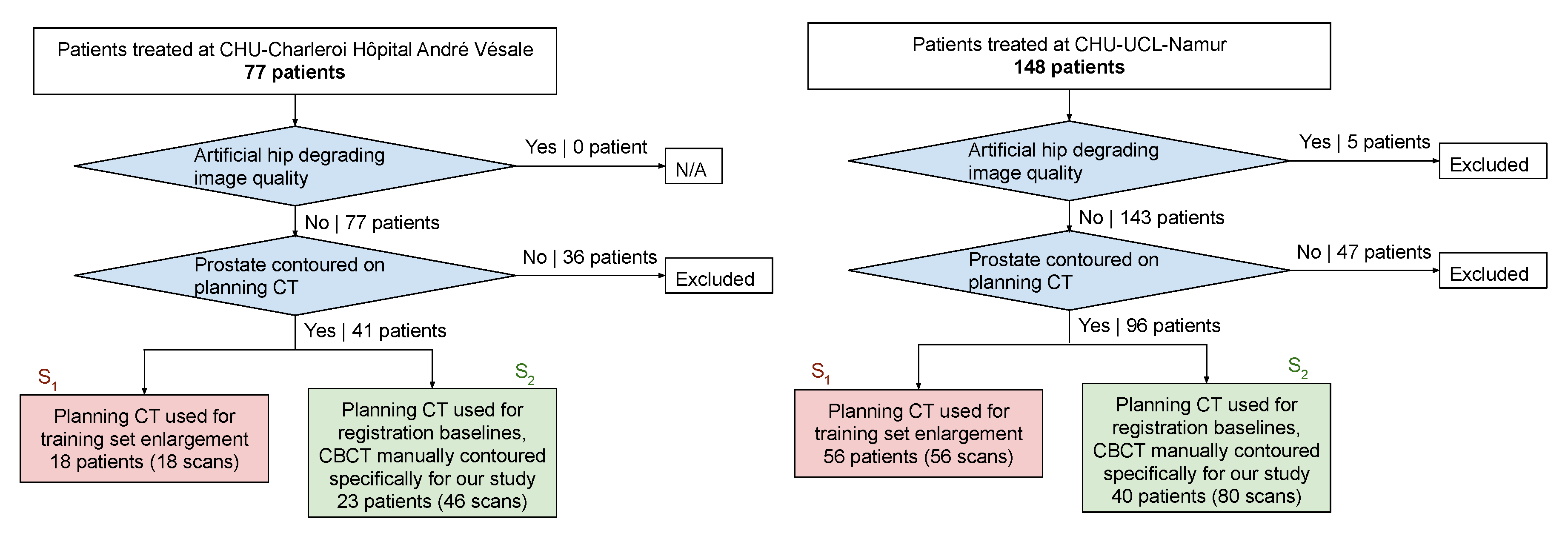
Our data consisted of (i) a set $S_1$ of 74 patients for whom we had delineated CT scans and (ii) a set $S_2$ of 63 patients (different from the 74 patients mentioned above) for whom we had delineated planning CT scans and delineated daily CBCT scans. The contours of bladder, rectum, and prostate were delineated on the CT scans during the clinical workflow. The contours on the CBCT scans were delineated by a trained expert specifically for this study. Within set $S_1$, 18 and 56 patients underwent EBRT for prostate cancer at two teaching hospitals, CHU-Charleroi Hôpital André Vésale and CHU-UCL-Namur, respectively. Within set $S_2$, 23 and 40 patients underwent EBRT for prostate cancer at CHU-Charleroi Hôpital André Vésale (CBCT scans acquired with a Varian TrueBeam STx version 1.5) and CHU-UCL-Namur (CBCT scans acquired with a Varian OBI cone beam CT), respectively. The use of these retrospective, anonymized data for this study was approved by each hospital’s ethics committee (dates of approval: 24 May 2017 for CHU-Charleroi Hôpital André Vésale and 12 May 2017 for CHU-UCL-Namur). In order to ensure data uniformity across the entire dataset, all 3D CT and CBCT scans (as well as the 3D binary masks representing the manual segmentations) were re-sampled on a 1.2 × 1.2 × 1.5 $\mathrm{m}\mathrm{m}$ regular grid. All re-sampled image volumes and binary mask volumes were cropped to volumes of 160 × 160 × 128 voxels containing bladder, rectum, and prostate.

The case selection procedure is described in Figure 2. Patients with an artificial hip were excluded from this study because the presence of an artificial hip degraded the image too much for the organs to be segmented accurately by a human expert. Patients for whom prostate was not contoured on the planning CT scan were also excluded. This corresponded to patients for whom the clinical target volume (CTV) differed from that of prostate, either because this organ had been surgically removed or because the CTV included other areas in addition to prostate. Note that it is common in radiotherapy to inject contrast media into bladder. Different inter-subject levels of contrast product increased the variability of this organ’s appearance, making its automatic contouring more challenging. Since our case selection procedure included all patients regardless of the use of contrast media, our method was supposed to be robust to such variability.

2.2. Model Architecture and Learning Strategy

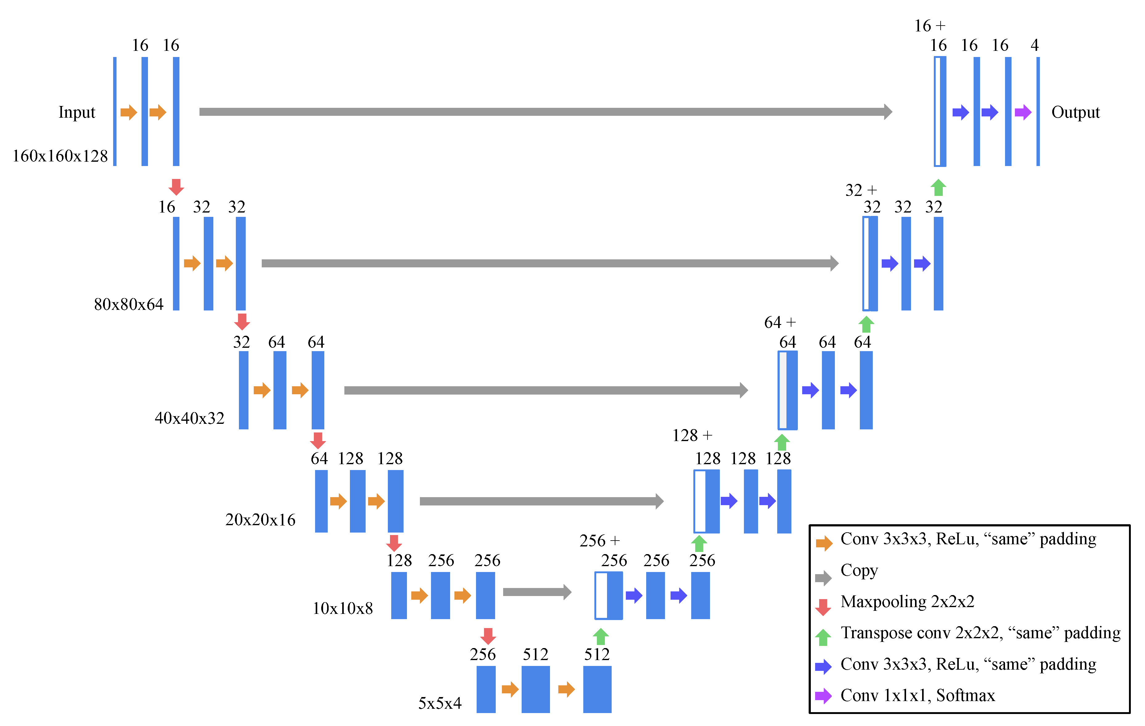
Bladder, rectum, and prostate were segmented on CBCT scans using the 3D U-net fully convolutional neural network [21,26]. The 3D input went through a contracting path to capture context and an expanding path to enable precise localization. In the last layer, a softmax was applied, and the network outputs the probability of each voxel belonging to bladder, rectum, prostate, or none of these organs. The network architecture is shown in Figure 3. To obtain a binary mask for each organ, the most probable class label was assigned to each pixel individually. In practice, each organ was segmented as a single region of connected voxels. No disconnected region of the same organ was observed. The main advantage of fully convolutional neural networks is that they output predictions at the same resolution as the input. One output channel was considered per organ. The network was trained with the Dice loss. The Adam optimization algorithm was used with a learning rate of ${10}^{-4}$. The number of epochs was chosen such that convergence was reached. The hyper-parameters mentioned here were the same as in Brion et al. [24] and proved satisfactory on the data used in this work. For this reason and to keep data available for training and testing, no validation set was considered here. Training data were augmented online using rotation (between $-5^{\circ }$ and $5^{\circ }$ along each of the three axes), shift (between −5 and 5 pixels along each axes), and shear (reasonable values for the affine transformation matrix). The batch size was set to two, which was the maximum size affordable on our 11 Gb graphical processing units (GPU).

We performed 3-fold cross-validation with the 63 CBCT scans of set ${\mathcal{S}}_2$, where 2 folds ($n_{CBCT}\le 42$ volumes in total) were used as the training set and one fold (21 volumes) as the test set, as shown in

Table 1. Three-fold cross-validation. To train the model, we used $n_{CT}$ CT scans from ${\mathcal{S}}_1$ and the $n_{CBCT}$ first volumes from the CBCT folds labeled “train.” To test the model, we used all 21 volumes from the CBCT fold labeled “test.”

${\mathcal{S}}_1$ (CT)	${\mathcal{S}}_2$ (CBCT)
	fold 1	fold 2	fold 3
train	train	train	test
train	train	test	train
train	test	train	train

. The number of training CBCT scans $n_{CBCT}$ was varied such that $n_{CBCT}\in \{0,6,10,20,30,42\}$. The training set was augmented with $n_{CT}$ annotated CT scans from set ${\mathcal{S}}_1$ such that $n_{CT}\in \{0,20,74\}$. The same CT scans were added to the training CBCT scans independently of the considered training folds. Hence, the training set contained $n_{CBCT}+n_{CT}$ volumes in total. Note that the test set contained no CT scans (since our goal was to segment CBCT scans only). The source code is publicly available at https://github.com/eliottbrion/pelvis_segmentation.

2.3. Validation and Comparison Baselines

In order to evaluate our contouring results, we used four metrics comparing the predicted and manual segmentations. The Dice similarity coefficient (DSC) and the Jaccard index (JI) measure the overlap between two binary masks, while the symmetric mean boundary distance (SMBD) assesses the distance between the contours (i.e., the sets of points located at the boundary of the binary masks) delineating those binary masks. We also computed the difference between the manual and predicted volumes for all the organs considered. More specifically,

$$\mathrm{DSC}=\frac{2|M\cap P|}{\left|M\right|+\left|P\right|},$$

(1)

$$\mathrm{JI}=\frac{|M\cap P|}{|M\cup P|},$$

(2)

$$\mathrm{SMBD}=\frac{\overline{D}(M,P)+\overline{D}(P,M)}{2},$$

(3)

where M and P are the sets containing the matricial indices of the manual and predicted segmentation 3D binary masks, respectively; $\overline{D}(M,P)$ is the mean of $D(M,P)$ over the voxels of ${\mathsf{\Omega }}_M$; and $D(M,P)=\left\{{min}_{x\in {\mathsf{\Omega }}_P}\right||s\odot (x-y)||,y\in {\mathsf{\Omega }}_M\}$, where ${\mathsf{\Omega }}_M$, ${\mathsf{\Omega }}_P$ are the boundaries extracted from M and P, respectively, and $s^{\top }=(1.2,1.2,1.5)$ is the pixel spacing in $\mathrm{m}$$\mathrm{m}$. Comparing the manual and predicted organ volumes was motivated by the field of application of this study. Indeed, from the perspective of adaptive radiotherapy, the organs’ volumes are needed in order to compare the initial CT plan dose-volume histograms for bladder, rectum, and prostate with the doses actually delivered as determined from CBCT scans acquired during the image-guided treatment [27]. The manual and predicted organ volumes were compared using a Bland–Altman plot, which allows quantification of the agreement between two quantitative measurements (i.e., the manual and predicted organ volumes) by studying their mean difference and constructing limits of agreement [28]. We computed the bias as:

$$\mathrm{Bias}=\frac{1}{n}\sum _{i=1}^n(p_i-m_i),$$

(4)

where n is the number of patients in the test set and $p_i=s_1\times s_2\times s_3\times \left|P_i\right|$, $m_i=s_1\times s_2\times s_3\times \left|M_i\right|$ are the volumes of the manual and predicted segmentations of the $i^{\mathrm{th}}$ patient. It provides the systematic under- or over-estimation of the predicted volumes. We also computed the precision,

$$\mathrm{Precision}=\frac{1}{n}\sum _{i=1}^n|p_i-m_i|,$$

(5)

which measures the difference between manual and predicted volume (in absolute value).

The DL-based segmentation was compared with different alternative approaches as summarized in

Table 2. DSC, JI, and SMBD, between the manual contours and the output of our proposed algorithm in different settings (number of training CBCT scans, number of training CT scans) for bladder, rectum, and prostate. Comparison with other benchmarking algorithms. Best results are presented in bold for our simulations and the state-of-the-art. DL: deep-learning, RS: RayStation, DSC: Dice similarity coefficient, JI: Jaccard index, SMBD: symmetric mean boundary distance, DIR: deformable image registration, PSM: patient specific model. * Evaluated on a dataset different from ours. ${}^{†}$ Results reported on a test set containing both CBCT and CT scans. ${}^{‡}$ The authors computed the root mean squared boundary distance rather than the SMBD. ${}^{\S }$ The authors computed the mean boundary distance and not the SMBD.

Study	Method	DSC			JI			SMBD (mm)
		Bladder	Rectum	Prostate	Bladder	Rectum	Prostate	Bladder	Rectum	Prostate
Ours	DL ($n_{CBCT}=20,n_{CT}=0$)	0.796 ± 0.128	0.680 ± 0.117	0.651 ± 0.158	0.677 ± 0.153	0.526 ± 0.123	0.501 ± 0.164	3.94 ± 2.18	3.85 ± 1.39	4.90 ± 2.85
Ours	DL ($n_{CBCT}=20,n_{CT}=74$)	0.846 ± 0.120	0.776 ± 0.068	0.708 ± 0.142	0.749 ± 0.155	0.638 ± 0.086	0.565 ± 0.157	3.02 ± 2.26	3.14 ± 1.43	3.87 ± 2.19
Ours	DL ($n_{CBCT}=42,n_{CT}=0$)	0.864 ± 0.096	0.773 ± 0.075	0.725 ± 0.139	0.771 ± 0.131	0.636 ± 0.098	0.585 ± 0.151	2.77 ± 1.95	3.06 ± 1.55	3.51 ± 2.03
Ours	DL ($n_{CBCT}=42,n_{CT}=74$)	0.874 ± 0.096	0.814 ± 0.055	0.758 ± 0.101	0.787 ± 0.131	0.690 ± 0.077	0.620 ± 0.120	2.47 ± 1.93	2.38 ± 0.98	3.08 ± 1.48
DIR	Rigid image registration	0.714 ± 0.149	0.646 ± 0.090	0.730 ± 0.108	0.576 ± 0.175	0.484 ± 0.102	0.585 ± 0.124	6.93 ± 4.09	5.30 ± 1.91	3.81 ± 1.44
DIR	DIR, RS intensity-based	0.737 ± 0.155	0.662 ± 0.100	0.739 ± 0.110	0.606 ± 0.187	0.504 ± 0.115	0.597 ± 0.127	6.27 ± 4.08	5.08 ± 2.04	3.61 ± 1.42
DIR	DIR, morphons	0.784 ± 0.151	0.684 ± 0.158	0.734 ± 0.127	0.668 ± 0.182	0.539 ± 0.165	0.594 ± 0.143	5.04 ± 3.90	5.00 ± 3.43	3.65 ± 1.64
Schreier et al. (2019) [25] *	DL ($n_{CBCT}$ = 300, $n_{CT}$ = 300)	0.932 ${}^{†}$	0.871 ${}^{†}$	0.840 ${}^{†}$	-	-	-	2.57  ±  0.54 ${}^{†,‡}$	2.47  ±  0.64${}^{†,‡}$	2.34  ±  0.68 ${}^{†,‡}$
Brion et al. (2019) [24] *	DL ($n_{CBCT}$ = 32, $n_{CT}$ = 64)	0.848  ±  0.085	-	-	0.745  ±  0.114	-	-	2.8  ±  1.4	-	-
Hänsch et al. (2018) [22] *	DL ($n_{CBCT}$ = 124, $n_{CT}$ = 88)	0.88	0.71	-	-	-	-	-	-	-
Motegi et al. (2019) [9] *	DIR, MIM intensity-based	∼ 0.80	∼ 0.40	∼ 0.55	-	-	-	-	-	-
Motegi et al. (2019) [9] *	DIR, RS intensity-based	∼ 0.78	∼ 0.70	∼ 0.75	-	-	-	-	-	-
Takayama et al. (2017) [10] *	DIR, RS intensity-based	0.69  ±  0.07	0.75  ±  0.05	0.84  ±  0.05	-	-	-	-	-	-
Woerner et al. (2017) [15] *	DIR, cascade MI-based	∼ 0.83	∼ 0.77	∼ 0.80	-	-	-	∼2.6 ${}^{\S }$	∼2.3 ${}^{\S }$	∼2.3 ${}^{\S }$
Konig et al. (2016) [16] *	DIR, rigid on bone and prostate	0.85  ±  0.05	-	0.82  ±  0.04	-	-	-	-	-	-
Thor et al. (2011) [12] *	DIR, demons	0.73	0.77	0.80	-	-	-	-	-	-
van de Schoot et al. (2014) [18] *	Patient specific model	∼ 0.87	-	-	-	-	-	-	-	-
Chai et al. (2012) [17] *	Patient specific model	0.78	-	-	-	-	-	-	-	-

. Two segmentation methods based on deformable image registration (denoted DIR in Table 2, second column) were applied to our dataset. First, the contours from the planning CT scans of set ${\mathcal{S}}_2$ were mapped to the follow-up CBCT scans of the same patient by using a rigid registration followed by DIR with the anatomically constrained deformation algorithm (ANACONDA) algorithm without controlling regions of interest (ROIs) in RayStation (https://www.raysearchlabs.com/raystation/) (Version 5.99.50.22) [29]. This algorithm adopts an intensity-based registration. Second, the contours were mapped from the planning CT scan to the follow-up CBCT scan using the diffeomorphic morphons’ DIR algorithm implemented in OpenReggui (https://openreggui.org/) [30]. This method exploits the local phase of the image volumes to perform the registration. Therefore, it is suited for registering image volumes with different contrast enhancement, such as CT and CBCT scans. The diffeomorphic version of the algorithm forces anatomically plausible deformations. We also compared our DL method with the Mattes mutual information rigid registration algorithm [31], as implemented in OpenReggui.

3. Results

In this section, we assess the performance of our algorithm in terms of overlap (i.e., DSC and JI), distance (i.e., SMBD), and volume agreement measurements. In the first part, we compare the overlaps and distances measured between our algorithm in different settings and the considered DIR-based segmentation approaches. In the second part, we further evaluate the performance of our best algorithm (i.e., 3D U-net trained with all available CT and CBCT scans) by assessing whether the predicted organ volumes are in good agreement with the volumes determined by manual segmentation. This was done by Bland–Altman analysis.

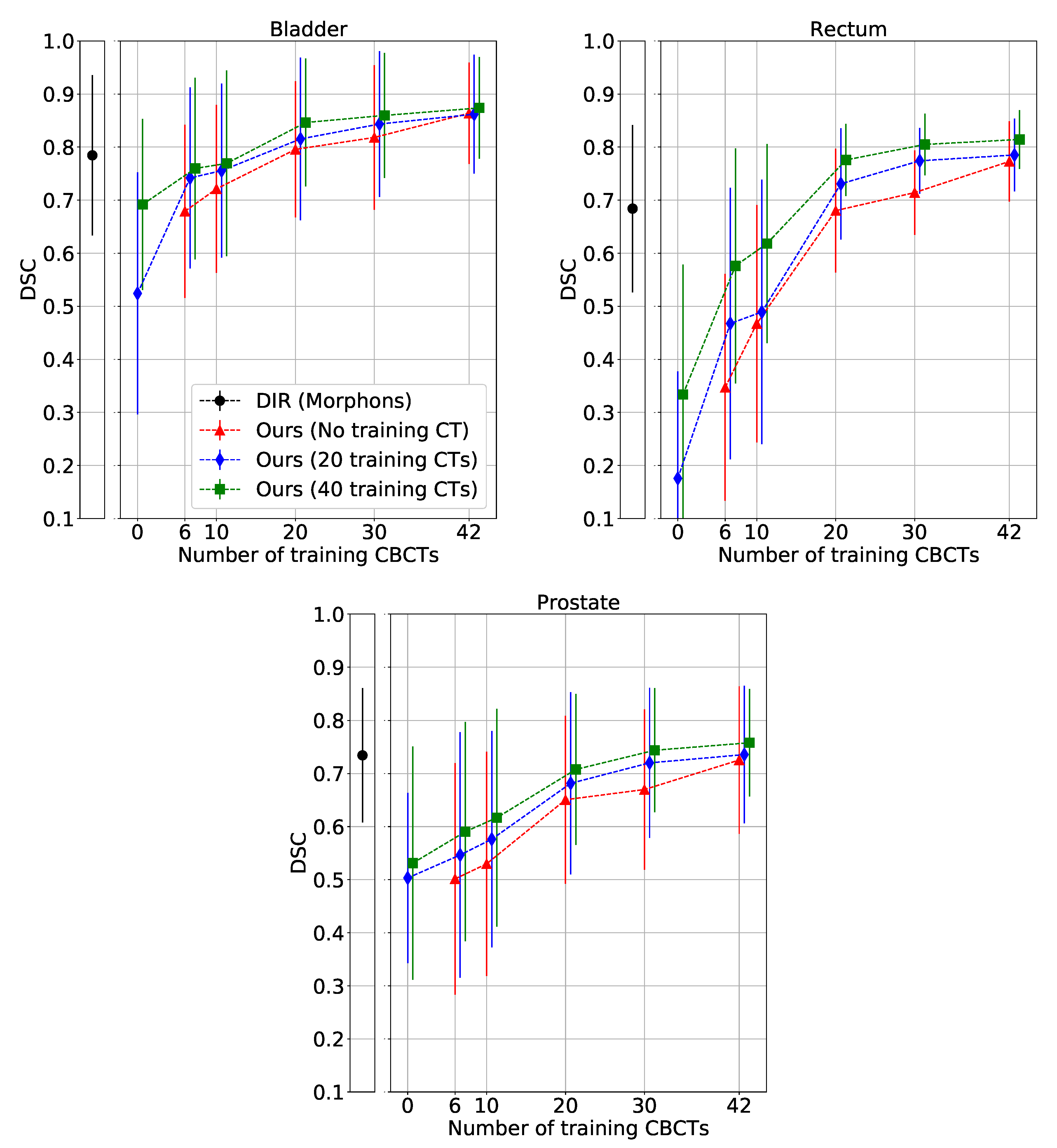
In Figure 4, the DSCs between the segmentation output of the fully convolutional neural network (FCN) and the ground truth segmentation were computed and averaged over all 63 CBCT scans from the three test folds. This was done for different numbers of training CBCT and CT scans. The results were then compared with the RayStation DIR algorithm, the diffeomorphic morphons’ algorithm, and rigid registration. Table 2 completes the plots in Figure 4 by providing the means and standard deviations of DSC, JI, and SMBD for different numbers of training CBCT scans and different numbers of training CT scans. The statistical model used for comparing the performances was a mixed model with a random intercept on the patient. It showed significant differences between algorithms’ performance for all organs regarding their DSC (bladder, rectum, prostate $p<{10}^{-3}$), JI (bladder, rectum, prostate $p<{10}^{-3}$), and SMBD (bladder, rectum, prostate $p<{10}^{-3}$). In the following paragraphs, the notation Ours($n_{CBCT}$, $n_{CT}$) stands for the 3D U-net proposed in this study with $n_{CBCT}$ CBCT scans and $n_{CT}$ CT scans in the training set. The p-values provided below were obtained by performing a Tukey’s range test on the DSCs. The following observations can be made based on Figure 4 and Table 2.

First, CBCT scans were more valuable than CT scans to train a CBCT segmentation model. This was not surprising and supported by the observation that a model trained on 40 CBCT and 0 CT scans performed significantly better than a model trained on 0 CBCT and 40 CT scans for all organs (bladder, rectum, prostate $p<{10}^{-3}$). The DSCs reached 0.634, 0.286, and 0.525 with Ours(0, 40) and 0.845, 0.754, and 0.722 with Ours(40, 0), for bladder, rectum, and prostate, respectively. Furthermore, a model trained only on 74 CT scans reached approximately the same performance as a network trained on only six to 10 CBCT scans for all the organs. Moreover, the more CBCT scans there were in the training set, the higher the DSCs on the test set were. This result made sense since adding new CBCT scans to the training set allowed the network to generalize on the test set (exclusively composed of CBCT scans) better. More surprisingly, we observed that once a sufficient number (typically 20) of CBCT scans were part of the training set, the benefit of adding CBCT or CT scans was practically the same. Indeed, compared with a model trained on 20 CBCT and 20 CT scans, the model trained on 40 CBCT and 0 CT scans did not lead to a significant improvement in performance (bladder $p=0.877$, rectum $p=0.700$, prostate $p=0.629$). The DSCs reached 0.815, 0.731, and 0.682 with Ours(20, 20) for bladder, rectum, and prostate, respectively. This confirmed that augmenting a CBCT training set with CT scans might be quite valuable.

Second, from the CT perspective, we clearly observed that the more CT scans there were in the training set, the higher the mean DSC became. Indeed, Ours(20, 74) was significantly better than Ours(20, 0) for all organs (bladder, rectum $p<{10}^{-3}$, prostate $p<{10}^{-2}$). We explained this improvement by the learning of more generic features, leading to better generalization. However, we observed that the difference in the average DSC between Ours(20, 0) and Ours(20, 20) was approximately equal to the difference the in average DSC between Ours(20, 20) and Ours(20, 74), whereas 20 new CT scans were added to the training set in the first case and 54 new CT scans in the second case. This may indicate saturation of the performance improvement produced by adding CT scans to the training set. Moreover, when the number of training CBCT scans was large, adding training CT scans improved performance for rectum only ($p<{10}^{-2}$): no statistically significant incremental change in performance was observed for bladder or prostate ($p=0.780$ and $p=0.630$, respectively) when Ours(42, 74) and Ours(42, 0) were compared. A plausible interpretation was that most of the useful information present in the CT scans was already captured in the relatively large CBCT training set. More importantly, in line with our objective of limiting the annotation of CBCT scans, we observed that the performance obtained with 42 CBCT and 0 CT scans could be reached with 20 CBCT and 74 CT scans for all organs (bladder $p=0.940$, rectum $p=0.882$, prostate $p=0.994$). Hence, the availability of 74 annotated CT scans reduced the number of annotated CBCT scans significantly (by a factor of approximately two).

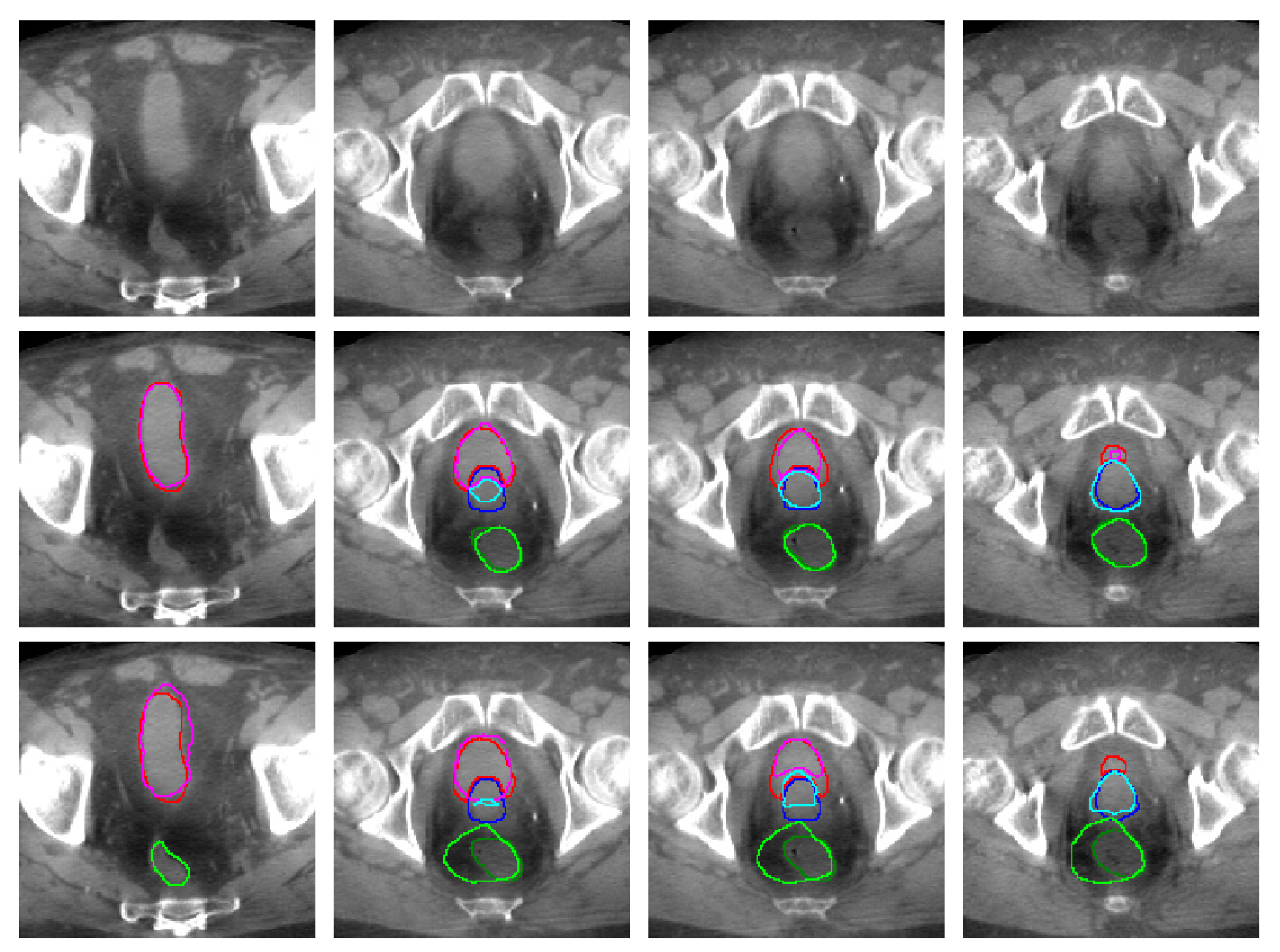
Third, when all available CT and CBCT scans (42 CBCT and 74 CT scans) were used for training, our approach significantly outperformed the rigid registration, RayStation DIR algorithm, and diffeomorphic morphons’ algorithm for bladder and rectum ($p<{10}^{-3}$), but not for prostate ($p=0.911$). These conclusions are illustrated on a representative patient in Figure 5. The results also showed that the rigid registration was outperformed by the ANACONDA algorithm, which was in turn outperformed by the diffeomorphic morphons’ algorithm for bladder and rectum. As mentioned above, both DIR methods were statistically similar to the rigid registration approach when it came to segmenting prostate. This supported the hypothesis that prostate underwent less deformation than bladder and rectum, which were subject to regular influxes and voiding of matter. Although our analysis was based on the DSC, both JI and SMBD led to the same conclusions.

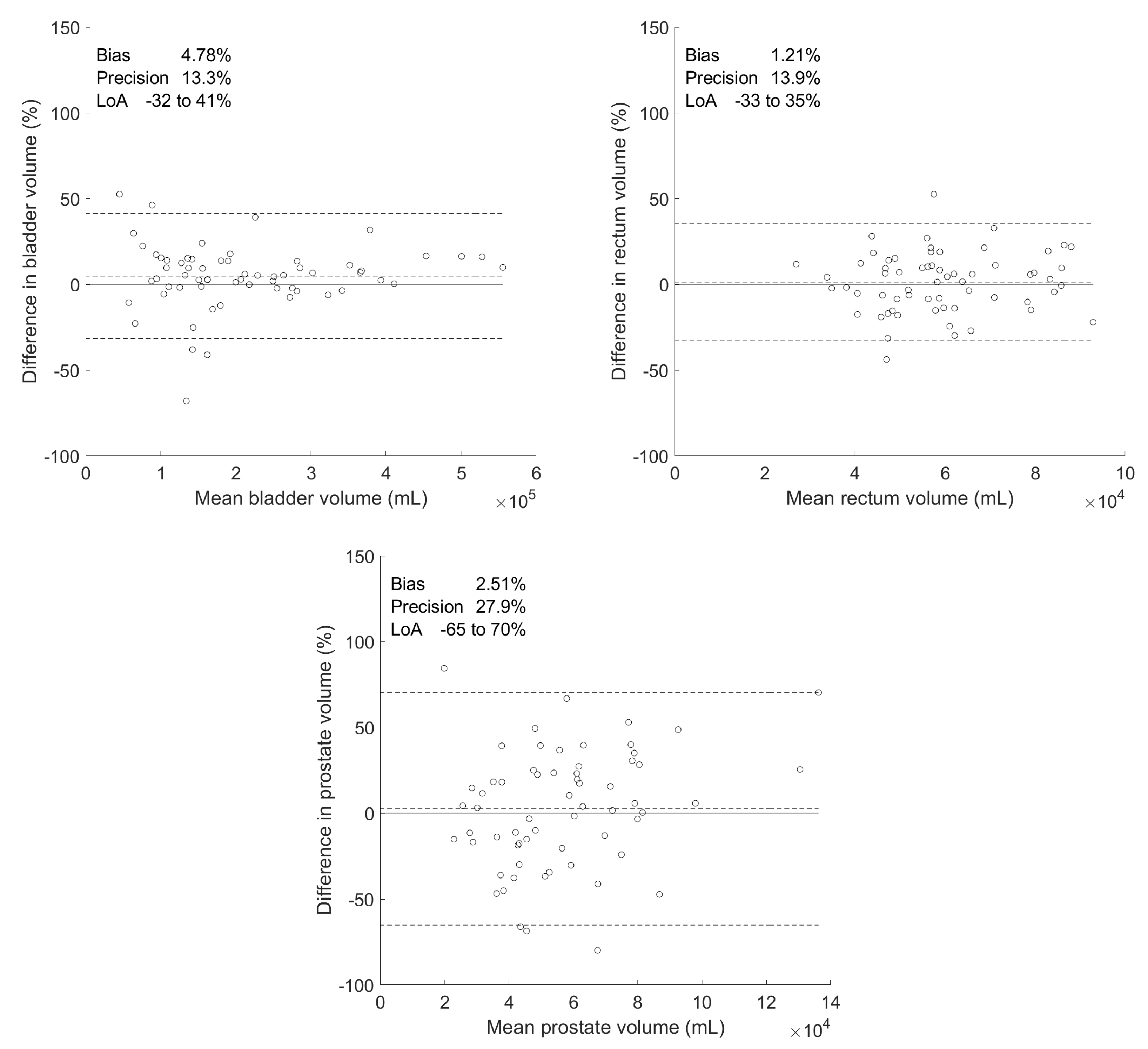
Figure 6 presents Bland–Altman plots comparing the organ volumes reached manually and by our DL-based predictions (obtained with Ours(42, 74)), using the bias, precision, and 95% limits of agreements (LoA). The bias normalized by the manual volume was below 5 % for all organs (bladder 4.78%, rectum 1.21%, prostate 2.51%). The precision normalized by the manual volume was similar for bladder and rectum (bladder 13.3%, rectum 13.9%) and larger for prostate (27.9%). The LoA of bladder were also close to the LoA of rectum (−32% and 41% for bladder and −33% and 35% for rectum), whereas they were larger for prostate (−65% and 70%).

Table 3. Absolute and relative differences between manual and predicted organs volumes. p-values are calculated using a one-sample t-test on percentage differences.

			Differences between Manual and Predicted Volumes
Organ	Volumes ($\times {10}^4\mathbf{m}\mathbf{L}$)		Absolute ($\times {10}^4\mathbf{m}\mathbf{L}$)		Percentage (%)
	Manual	Predicted	Bias	Precision	Bias	Precision	p-Value
Bladder	21.9  ±  12.9	20.7  ±  11.4	1.18	2.46	4.78	13.3	0.285
Rectum	5.96  ±  1.66	5.87  ±  1.55	0.094	0.826	1.21	13.9	0.897
Prostate	5.87  ±  2.98	5.53  ±  2.07	0.340	1.64	2.51	27.9	0.438

completes the Bland–Altman plots by providing the means and standard deviations for the manual and predicted organ volumes. Moreover, a one-sample t-test was performed on the differences between the manual and predicted volumes normalized by the manual volume for each organ. The resulting p-values for all organs are presented in Table 3 and were not significantly different (bladder $p=0.285$, rectum $p=0.897$, prostate $p=0.438$). This meant that the predicted and manual contours were similar in means according to the t-test.

Computational cost analysis was performed by measuring the running time on our machine equipped with an 11Gb GeForce GTX 1080 Ti graphics card. The rigid registration of one image ran in 1.05 $\min$. The deformable image registration with the ANACONDA and morphons’ algorithms ran in 1.92 $\min$ and 8.33 $\min$, respectively. The inference time for one image with the DL approaches was much lower. It reached 0.15 $\mathrm{s}$ independently of the learning strategy. Indeed, the number of images in the training set had no impact on the inference time. The training time needed to reach convergence depended on the size of the training set. Hence, Ours(20, 0), Ours(20, 74), Ours(42, 0), and Ours(42, 74) were trained in 17.3, 224, 167, and 220 $\min$, respectively.

4. Discussion

Based on Table 2 (first part) and Figure 4, the 3D U-net approach was the most satisfactory approach for automatic segmentation of bladder and rectum on CBCT scans. This supported the initial hypothesis that registration-based approaches failed in the case of large deformation and alternative approaches using the statistics of the target image (i.e., the CBCT scan) were more suitable. This observation was also consistent with the state-of-the-art algorithms shown in Table 2 (second part), where DL approaches outperformed alternative approaches for bladder and rectum.

Still based on Table 2 (first part) and Figure 4, the 3D U-net slightly outperformed the registration-based approaches for prostate, but this improvement was not statistically significant. 3D U-net’s lower performances for prostate than for bladder and rectum was further supported by the Bland–Altman analysis of the manual and predicted volumes. Indeed, this analysis provided less than 5% bias for all organs, but higher precision (i.e., a larger spread of the predictions, as defined in (5)) for prostate than for bladder and rectum. Furthermore, most other state-of-the-art DIR-based algorithms outperformed our approach for prostate. This showed that DIR-based approaches were still valuable in situations with limited organ deformation and where poor contrast made the use of vanilla DL models challenging. A first way to improve the segmentation results for prostate and outperform DIR-based approaches without annotating more CBCT scans might be to generate pseudo CBCT scans as in Schreier et al., but our study showed that increasing the number of already annotated CT scans further was a valuable alternative, albeit with a risk of saturation. If few data are available, a second option could be to promote a desired shape or structure in the deep model prediction [32,33]. A third option could be to perform unsupervised domain adaptation [34]. This approach requires annotations in a source domain (CT), but not in the target domain (CBCT). This will be the subject of future research.

From an application point of view, the study showed that the more CBCT scans were contoured, the better the DSC on the predicted contours. However, contouring CBCT scans is not part of the clinical workflow, is time consuming, and is not easy because of the poor contrast between the different regions of interest. Hence, we showed that expanding the training set with CT scans improved the segmentation performances for all considered organs, especially when few contoured CBCT scans were available. Our 3D U-net that reached the best segmentation performances was trained with 42 CBCT and 74 CT scans.

Most cases of failure were observed for prostate, which had the lowest DSC of the organs. This may be due to the fact that prostate is hard to see on CBCT scans and often pushes on bladder, as we can see in Figure 5. Hence, some upper parts of prostate were often wrongly classified as bladder, which decreased the DSC for prostate. Since bladder is larger than prostate, misclassification at the boundary between the two organs had less impact on the DSC of bladder. A second case of failure occurred at the top and bottom slices of rectum, which was wrongly classified as the background (or inversely, the background was wrongly classified as rectum). This made sense since there were few differences in contrast between rectum, anal canal, and colon. The impact of such errors on prostate and rectum, as well as the required contour quality for clinical use in adaptive radiotherapy, was such that additional quality assessment with a contours review process was needed. This should be done by radiation oncologists and will be the subject of future research.

Our DL approach also outperformed or achieved the same performance as patient specific models for bladder. Those models rely on PCA to extract principal modes of deformation from landmarks placed on bladder’s contour and across several contoured images for each patient being considered. The drawback for clinical use of such approaches is that (i) a different model is required for every patient and organ and (ii) several images per patient are needed to build the model.

Concerning alternative DL methods, the current work slightly outperformed our initial conference paper, Brion et al. [24], on bladder segmentation with 3D U-net. This was probably due to the larger training database and/or the multi-class formulation used in this work, since three organs were segmented instead of one. Only 41 of the patients used in our conference paper were kept in this study. This was because the remaining patients had either had their prostates removed or lacked fully annotated scans. New patients were also added. The two datasets were thus different. However, Schreier et al.’s work was the closest to this study. Hence, we did a more thorough comparison with their findings. They obtained a higher DSC than we did for all the organs considered in this study. This might be explained by the fact that they used more samples in their training set (300 CT and 300 pseudo CBCT scans compared with 74 CT and 42 CBCT scans). However, it was hard to determine whether this was the only explanation for their better results. Indeed, in Figure 4, we see that the DSC increased more slowly as the number of training samples increased. Interestingly, they ran the patch-wise 3D U-net proposed by Hänsch et al. on their test set and obtained DSCs of 0.927, 0.860, and 0.816 for bladder, rectum, and prostate, respectively. Those results were higher than the results obtained on bladder (DSC = 0.88) and rectum (DSC = 0.71) by Hänsch et al. Therefore, their test set might be of a higher quality than ours, which could be a limitation of their approach in clinical practice, where low quality images are common. Another shortcoming is that they reported their results on a dataset that included both CBCT and CT scans (10%). It was therefore unclear how well their method would perform on a dataset containing only CBCT scans (such as ours). As a final remark, their proposed generation of pseudo CBCT scans from clinically contoured CT scans was a powerful tool for solving the problem of CBCT annotations. However, such knowledge of artificial data generation might not be present in all hospitals. To summarize this comparison, we considered the two publications to be complementary, with our strengths being the size of our test set, detailed comparison with registration approaches, and the detailed study of the impact of additional CT scans in the training database.

5. Conclusions

In this work, a 3D U-net DL model was trained on CBCT an CT scans in order to segment bladder, rectum, and prostate on CBCT scans. The proposed approach significantly outperformed all the DIR-based segmentation methods applied on our dataset in terms of DSC, JI, and SMBD for bladder and rectum. The conclusions were more mitigated concerning prostate, where the DL-based segmentation did not significantly outperform alternative approaches. A Bland–Altman analysis on the manual and predicted organs’ volumes revealed a low bias on the predicted volumes for all organs, but higher precision (i.e., a larger spread of the volumes) for prostate than for the other organs. Furthermore, the study showed that the cross-domain data augmentation consisting of adding CT to the CBCT scans in the training set significantly improved the segmentation results. A further step will be to highlight these improvements by showing the better tumor coverage and reduction in the doses delivered to organs at risk that it allows.

References

1. Brousmiche, S.; Orban de Xivry, J.; Macq, B.; Seco, J. SU-E-J-125: Classification of CBCT Noises in Terms of Their Contribution to Proton Range Uncertainty. Med. Phys. 2014, 41, 184. [Google Scholar] [CrossRef]
2. Peng, C.; Ahunbay, E.; Chen, G.; Anderson, S.; Lawton, C.; Li, X.A. Characterizing interfraction variations and their dosimetric effects in prostate cancer radiotherapy. Int. J. Radiat. Oncol. Biol. Phys. 2011, 79, 909–914. [Google Scholar] [CrossRef] [PubMed]
3. Ghilezan, M.; Yan, D.; Martinez, A. Adaptive Radiation Therapy for Prostate Cancer. Semin. Radiat. Oncol. 2010, 20, 130–137. [Google Scholar] [CrossRef] [PubMed] [Green Version]
4. Pos, F.; Remeijer, P. Adaptive Management of Bladder Cancer Radiotherapy. Semin. Radiat. Oncol. 2010, 20, 116–120. [Google Scholar] [CrossRef]
5. Wang, Y.; Efstathiou, J.A.; Sharp, G.C.; Lu, H.M.; Ciernik, I.F.; Trofimov, A.V. Evaluation of the dosimetric impact of interfractional anatomical variations on prostate proton therapy using daily in-room CT images. Med. Phys. 2011, 38, 4623–4633. [Google Scholar] [CrossRef] [Green Version]
6. Moteabbed, M.; Trofimov, A.; Sharp, G.C.; Wang, Y.; Zietman, A.L.; Efstathiou, J.A.; Lu, H.M. Proton therapy of prostate cancer by anterior-oblique beams: Implications of setup and anatomy variations. Phys. Med. Biol. 2017, 62, 1644–1660. [Google Scholar] [CrossRef] [Green Version]
7. Rigaud, B.; Simon, A.; Castelli, J.; Lafond, C.; Acosta, O.; Haigron, P.; Cazoulat, G.; de Crevoisier, R. Deformable image registration for radiation therapy: Principle, methods, applications and evaluation. Acta Oncol. 2019, 58, 1225–1237. [Google Scholar] [CrossRef]
8. Oh, S.; Kim, S. Deformable image registration in radiation therapy. Radiat. Oncol. J. 2017, 35, 101. [Google Scholar] [CrossRef]
9. Motegi, K.; Tachibana, H.; Motegi, A.; Hotta, K.; Baba, H.; Akimoto, T. Usefulness of hybrid deformable image registration algorithms in prostate radiation therapy. J. Appl. Clin. Med. Phys. 2019, 20, 229–236. [Google Scholar] [CrossRef] [Green Version]
10. Takayama, Y.; Kadoya, N.; Yamamoto, T.; Ito, K.; Chiba, M.; Fujiwara, K.; Miyasaka, Y.; Dobashi, S.; Sato, K.; Takeda, K.; et al. Evaluation of the performance of deformable image registration between planning CT and CBCT images for the pelvic region: Comparison between hybrid and intensity-based DIR. J. Radiat. Res. 2017, 58, 567–571. [Google Scholar] [CrossRef]
11. Zambrano, V.; Furtado, H.; Fabri, D.; Lütgendorf-Caucig, C.; Góra, J.; Stock, M.; Mayer, R.; Birkfellner, W.; Georg, D. Performance validation of deformable image registration in the pelvic region. J. Radiat. Res. 2013, 54, i120–i128. [Google Scholar] [CrossRef] [PubMed] [Green Version]
12. Thor, M.; Petersen, J.B.; Bentzen, L.; Høyer, M.; Muren, L.P. Deformable image registration for contour propagation from CT to cone-beam CT scans in radiotherapy of prostate cancer. Acta Oncol. 2011, 50, 918–925. [Google Scholar] [CrossRef] [PubMed]
13. Söhn, M.; Birkner, M.; Chi, Y.; Wang, J.; Yan, D.; Berger, B.; Alber, M. Model-independent, multimodality deformable image registration by local matching of anatomical features and minimization of elastic energy. Med. Phys. 2008, 35, 866–878. [Google Scholar] [CrossRef] [PubMed]
14. Thirion, J.P. Image matching as a diffusion process: An analogy with Maxwell’s demons. Med. Image Anal. 1998, 2, 243–260. [Google Scholar] [CrossRef] [Green Version]
15. Woerner, A.J.; Choi, M.; Harkenrider, M.M.; Roeske, J.C.; Surucu, M. Evaluation of deformable image registration-based contour propagation from planning CT to cone-beam CT. Technol. Cancer Res. Treat. 2017, 16, 801–810. [Google Scholar] [CrossRef] [Green Version]
16. König, L.; Derksen, A.; Papenberg, N.; Haas, B. Deformable image registration for adaptive radiotherapy with guaranteed local rigidity constraints. Radiat. Oncol. 2016, 11, 122. [Google Scholar] [CrossRef] [Green Version]
17. Chai, X.; van Herk, M.; Betgen, A.; Hulshof, M.; Bel, A. Automatic bladder segmentation on CBCT for multiple plan ART of bladder cancer using a patient-specific bladder model. Phys. Med. Biol. 2012, 57, 3945. [Google Scholar] [CrossRef]
18. Van de Schoot, A.; Schooneveldt, G.; Wognum, S.; Hoogeman, M.; Chai, X.; Stalpers, L.; Rasch, C.; Bel, A. Generic method for automatic bladder segmentation on cone beam CT using a patient-specific bladder shape model. Med. Phys. 2014, 41, 031707. [Google Scholar] [CrossRef]
19. Kazemifar, S.; Balagopal, A.; Nguyen, D.; McGuire, S.; Hannan, R.; Jiang, S.; Owrangi, A. Segmentation of the prostate and organs at risk in male pelvic CT images using deep learning. arXiv 2018, arXiv:1802.09587. [Google Scholar] [CrossRef] [Green Version]
20. Cha, K.H.; Hadjiiski, L.; Samala, R.K.; Chan, H.P.; Caoili, E.M.; Cohan, R.H. Urinary bladder segmentation in CT urography using deep-learning convolutional neural network and level sets. Med. Phys. 2016, 43, 1882–1896. [Google Scholar] [CrossRef]
21. Çiçek, Ö.; Abdulkadir, A.; Lienkamp, S.S.; Brox, T.; Ronneberger, O. 3D U-Net: Learning dense volumetric segmentation from sparse annotation. In Proceedings of the International Conference on Medical Image Computing and Computer-Assisted Intervention, Athens, Greece, 17–21 October 2016; Springer: Berlin/Heidelberg, Germany, 2016; pp. 424–432. [Google Scholar]
22. Haensch, A.; Dicken, V.; Gass, T.; Morgas, T.; Klein, J.; Meine, H.; Hahn, H. Deep learning based segmentation of organs of the female pelvis in CBCT scans for adaptive radiotherapy using CT and CBCT data. Int. J. Comput. Assist. Radiol. Surg. 2018, 13, 179–180. [Google Scholar]
23. Hänsch, A.; Dicken, V.; Klein, J.; Morgas, T.; Haas, B.; Hahn, H.K. Artifact-driven sampling schemes for robust female pelvis CBCT segmentation using deep learning. In Medical Imaging 2019: Computer-Aided Diagnosis; International Society for Optics and Photonics: Bellingham, WA, USA, 2019; Volume 10950, p. 109500T. [Google Scholar]
24. Brion, E.; Léger, J.; Javaid, U.; Lee, J.; De Vleeschouwer, C.; Macq, B. Using planning CTs to enhance CNN-based bladder segmentation on cone beam CT. In Medical Imaging 2019: Image-Guided Procedures, Robotic Interventions, and Modeling; International Society for Optics and Photonics: Bellingham, WA, USA, 2019; Volume 10951, p. 109511M. [Google Scholar]
25. Schreier, J.; Genghi, A.; Laaksonen, H.; Morgas, T.; Haas, B. Clinical evaluation of a full-image deep segmentation algorithm for the male pelvis on cone-beam CT and CT. Radiother. Oncol. 2020, 145, 1–6. [Google Scholar] [CrossRef] [PubMed] [Green Version]
26. Ronneberger, O.; Fischer, P.; Brox, T. U-net: Convolutional networks for biomedical image segmentation. In Proceedings of the International Conference on Medical Image Computing and Computer-Assisted Intervention, Munich, Germany, 5–9 October 2015; Springer: Berlin/Heidelberg, Germany, 2015; pp. 234–241. [Google Scholar]
27. Hatton, J.A.; Greer, P.B.; Tang, C.; Wright, P.; Capp, A.; Gupta, S.; Parker, J.; Wratten, C.; Denham, J.W. Does the planning dose—Volume histogram represent treatment doses in image-guided prostate radiation therapy? Assessment with cone-beam computerised tomography scans. Radiother. Oncol. 2011, 98, 162–168. [Google Scholar] [CrossRef] [PubMed]
28. Giavarina, D. Understanding bland altman analysis. Biochem. Med. Biochem. Med. 2015, 25, 141–151. [Google Scholar] [CrossRef] [Green Version]
29. Weistrand, O.; Svensson, S. The ANACONDA algorithm for deformable image registration in radiotherapy. Med. Phys. 2015, 42, 40–53. [Google Scholar] [CrossRef]
30. Janssens, G.; Jacques, L.; de Xivry, J.O.; Geets, X.; Macq, B. Diffeomorphic registration of images with variable contrast enhancement. J. Biomed. Imaging 2011, 2011, 3. [Google Scholar] [CrossRef]
31. Mattes, D.; Haynor, D.R.; Vesselle, H.; Lewellen, T.K.; Eubank, W. PET-CT image registration in the chest using free-form deformations. IEEE Trans. Med. Imaging 2003, 22, 120–128. [Google Scholar] [CrossRef]
32. Oktay, O.; Ferrante, E.; Kamnitsas, K.; Heinrich, M.; Bai, W.; Caballero, J.; Cook, S.A.; De Marvao, A.; Dawes, T.; O‘Regan, D.P.; et al. Anatomically constrained neural networks (ACNNs): Application to cardiac image enhancement and segmentation. IEEE Trans. Med Imaging 2017, 37, 384–395. [Google Scholar] [CrossRef] [Green Version]
33. Ravishankar, H.; Venkataramani, R.; Thiruvenkadam, S.; Sudhakar, P.; Vaidya, V. Learning and incorporating shape models for semantic segmentation. In Proceedings of the International Conference on Medical Image Computing and Computer-Assisted Intervention, Quebec, QC, Canada, 11–13 September 2017; Springer: Berlin/Heidelberg, Germany, 2017; pp. 203–211. [Google Scholar]
34. Kamnitsas, K.; Baumgartner, C.; Ledig, C.; Newcombe, V.; Simpson, J.; Kane, A.; Menon, D.; Nori, A.; Criminisi, A.; Rueckert, D.; et al. Unsupervised domain adaptation in brain lesion segmentation with adversarial networks. In Proceedings of the International Conference on Information Processing in Medical Imaging, Boone, NC, USA, 25–30 June 2017; Springer: Berlin/Heidelberg, Germany, 2017; pp. 597–609. [Google Scholar]
Sample Availability: Access to the dataset is subjected to the authorization of the partner hospitals’ ethics committees. The dataset is not available by default.
Figure 1. Comparison of CT and CBCT scans
Applsci 10 01154 g001
Figure 2. Case selection from CHU-Charleroi Hôpital André Vésale and CHU-UCL-Namur.
Applsci 10 01154 g002
Figure 3. 3D U-net model architecture. Each blue rectangle represents the feature maps resulting from a convolution operation, while white rectangles represent copied feature maps. For the convolutions, zero padding was chosen such that the volume size was preserved (“same” padding). The output size was 4: one per segmentation (bladder, rectum, and prostate) and one for the background.
Applsci 10 01154 g003
Figure 4. Influence of the number of training CBCT and CT scans on the DSC. Bars indicate one standard deviation for the group of 63 patients. DSC: Dice similarity coefficient.
Applsci 10 01154 g004
Figure 5. Comparison of manual, 3D U-net, and morphons’ DIR-based segmentation for a representative patient. Each column corresponds to a slice of the same CBCT scan. Dark colors represent reference segmentations (both second and third rows), while light colors show 3D U-net segmentation (second row) and morphons’ DIR-based segmentation (third row). The predicted bladder, in pink, has a DSC of 0.940 (U-net) and 0.864 (morphons); rectum, in light green, has a DSC of 0.791 and 0.759; prostate, in light blue, has a DSC of 0.780 and 0.730.
Applsci 10 01154 g005
Figure 6. Bland–Altman plots for bladder, rectum, and prostate derived from the differences between the predicted and manual segmentations. The solid lines represent no difference; the dotted lines depict the mean difference (bias) and 95% limits of agreements (LoA).
Applsci 10 01154 g006