An Online Reactive Power-Optimization Strategy Based on Load-Curve Prediction and Segmentation

Featured Application

Voltage Regulation in Distribution Systems.

Abstract

Due to fluctuating characteristics of loads, dynamic reactive power optimization over a certain time period is essential to provide effective strategies to maintain the security and economic operation of distribution systems. In operation, reactive power compensation devices cannot be adjusted too frequently due to their lifetime constraints. Thus, in this paper, an online reactive power optimization strategy based on the segmentation of multiple predicted load curves is proposed to address this issue, aiming to minimize network losses and at the same time to minimize reactive power-compensation device adjustment times. Based on forecasted time series of loads, the strategy first segments each load curve into several sections by means of thresholding a filtered signal, and then optimizes reactive power dispatch based on average load in each section. Through case studies using a modified IEEE 34-bus system and field measurement of loads, the merits of the proposed strategy is verified in terms of both optimization performance and computational efficiency compared with state-of-the-art methods.

1. Introduction

Reactive power optimization aims to produce optimal reactive power-compensation device control strategies in order to achieve minimum delivery losses and at the same time to satisfy specific operating constraints such as requirements for voltage deviations [1,2]. The problem in essence is a mixed-integer non-linear programming problem. Various optimization methods have been applied to address this issue, including linear programming [3], non-linear programming [4], quadratic programming [5], interior point programming [6,7], and artificial intelligence (AI) methods [2,8,9]. Reference [10] used second-order cones to relax the non-convex power flow equations, and then applied a sensitivity-based decomposition method to improve computational efficiency. Reference [11] transformed non-linear power flow equations into a linear approximation form, and used iterative solving algorithm to obtain optimal reactive power dispatch strategy. Reference [12] implemented genetic algorithm to maintain voltage stability of the power system and also to reduce power losses in systems with mass distributed generators.

The aforementioned research provided solutions for stable reactive power optimization, which optimizes based on certain load level at single time stamp. However, since power generation and loads are constantly variable, the optimal strategies for devices like voltage regulators or switchable capacitor banks may not be the same at different time stamps. Due to lifetime limitations of these devices, it violates the economic rule if the devices are adjusted too frequently. Therefore, dynamic reactive power optimization is of importance, which optimizes for a time period and makes the adjustment times of devices one of the optimization objectives.

Dynamic reactive power optimization is a large-scale multi-period mix-integer non-linear programming problem. The classical methods such as non-linear programming [4] require differentiable objective function and are thus not applicable for dynamic optimization.

A number of attempts have been made to conquer the problem of dynamic optimization. Reference [13] made daily reactive power optimization considering network losses, adjustment times of on-load tap changer (OLTC) and switchable capacitor banks, using an improved multi-population ant colony algorithm. Reference [14] used mixed integer non-linear programming to optimize transmission losses only, considering constraints of reactive power equipment operation limits and power grid security. Using a filter collaborative state transition algorithm (FCSTA), reference [15] built a two-objective dynamic reactive power optimization model, with one objective to minimize the actual power losses and voltage deviations, the other to minimize incremental system loss compared with the last time stamp. The objectives can be exchanged during dynamic optimization.

Generally, state-of-the-art attempts include reducing scales of objectives or constraints, optimizing for increments at continuous time stamp, and using AI methods. However, much computational burden will be introduced when using AI methodology.

Aiming to maintain objectives and constraints, as well as to reduce computational complexity, this paper proposes to segment load curves in a duty cycle into several stable time series first, and then conduct optimization for each segment. Based on online load predictions, the method can be applied in an online mode. Since the whole time series of loads need to be segmented into parts with lowest inner deviation, the methods of wind ramp extraction [16,17] are utilized to extract data points corresponding to big changes. The data points are afterwards used for segmentation.

This paper is organized as follows. The proposed load curve segmentation-based reactive power optimization is described in Section 2. In Section 3, two case studies, one based on offline load-curve measurements, the other based on online load predictions, are presented to evaluate the effectiveness of the proposed method. The discussion of the experimental results is described in Section 4. Section 5 presents conclusions and future work.

2. Reactive Power Optimization Based on Load-Curve Segmentation

2.1. Load-Curve Segmentation

When conducting reactive power optimization, the adjustment of reactive power compensation devices will change with the variations of loads. It is common that on a daily basis load levels in a certain period remain relatively stable. Peak load usually occurs at noon or in the evening. Therefore, it is possible to segment the load curve and hereafter to optimize only once for this certain time period using average load level.

In order to segment a load curve into sections with lowest inner deviation, the method of wind ramp detection [16,17] is used. A filtered curve is first derived to represent the magnitude of change around each time stamp. Two methods of filtering are introduced in this paper. In the first filtering method, the filtered curve calculates maximum load difference in neighboring time periods and at the same time ignoring any changes within that period [16]. In detail, the original load-curve time series $L_t$ can be transformed into a filtered representation $L_t^f$ as below.

$$L_t^f=\max (L(t:t+n))-\min (L(t:t+n))$$

(1)

In (1), the load curve is noted as $L(t)$, the filtered curve is written as $L_t^f$, and $n$ represents the time span of interest when considering changes.

The second filtering method [17], noted as method 2, refers to a different calculation of the filtered curve, as shown in (2).

$$L_t^f=mean\left\{L(t+h)-L(t+h-n);h=1,\dots n\right\}$$

(2)

In (2), a smaller $n$ indicates a shorter time period in consideration when judging changing of load curves, corresponding to relatively sharp load changes.

After deriving filtering curves, the time stamps corresponding to big load changes can be extracted using a threshold $L_{thr}$ as in (3).

$$t:\left|L_t^f\right|>L_{thr}$$

(3)

These time stamps can then be used as separation points for load curve segmentation. In detail, if more than two neighboring points are all above the threshold, those in the middle become independent sections themselves, and the two points on the edge are grouped with their neighbors below the threshold. If the neighbors of one separation point are all below the threshold, this point can be grouped with the neighbor who has relatively similar load value.

As for each section, the average load is calculated, and then be used for reactive power optimization for the time period of this section.

2.2. Segmentation in Case of Multiple Load Curves

Since the power consumption characteristics of different power consumers are not the same, it is not applicable to assume all consumers follow the single load curve. In case of multiple load curves, two strategies can be applied. One is to conduct segmentation for each load curve first, and use all separation points to do final segmentation.

Another alternative strategy is to use an integrated load curve. Suppose there exist $K$ users, each corresponding to independent load curve. Let $L_{t,k}$ be the load curve of $k$-th user, $P_k$ be the its capacity in kW, the integrated load curve $L_{total}$ can be calculated as below.

$$L_{total}={\displaystyle \sum _{k=1}^K{P}_k{L}_{t,k}}$$

(4)

Afterwards, the segmentation methods mentioned in previous section can be applied to the integrated load curve.

2.3. Reactive Power Optimization

For each time stamp, the changes of tap positions and capacitor banks are considered in the objective function, which can be written in (5).

$$\min f(t)=\alpha \cdot \frac{P_{loss,t}-P_{loss\_\min }}{P_{loss\_\max }-P_{loss\_\min }}+\beta \cdot \frac{\mathrm{\Delta }A{T}_t-\mathrm{\Delta }A{T}_{\min }}{\mathrm{\Delta }A{T}_{\max }-\mathrm{\Delta }A{T}_{\min }}$$

(5)

where $P_{loss,t}$ is network loss at time stamp $t$. For normalization, $P_{loss\_\min }$ and $P_{loss\_\max }$ represent basis values for network losses. $\mathrm{\Delta }A{T}_t$ indicates adjustment times of devices at current time stamp compared with the previous one [15], which can be written in (6). $\mathrm{\Delta }A{T}_{\min }$ and $\mathrm{\Delta }A{T}_{\max }$ are basis values for adjustment times. $\alpha$ and $\beta$ are optimization weights.

$$\mathrm{\Delta }A{T}_t={\displaystyle \sum _{m=1}^M(T{P}_{m,t}-T{P}_{m,t-1})}+{\displaystyle \sum _{k=1}^K(C_{k,t}-C_{k,t-1})}$$

(6)

In (6), $T{P}_{m,t}$ represents tap position of $m$-th voltage regulator at time $t$, and $C_{k,t}$ is capacitor number at time $t$.

Constraints include three categories, i.e., power flow constraints (7), bus voltage magnitudes not exceeding permissible range (8), and adjustment device state constraints (9) [15,18].

$$\begin{array}{l}{P}_{i,t}=V_{i,t}{\displaystyle \sum _{j=1}^N{V}_{j,t}(G_{ij}\cos {\theta }_{ij,t}+B_{ij}\sin {\theta }_{ij,t})}\\ Q_{i,t}=V_{i,t}{\displaystyle \sum _{j=1}^N{V}_{j,t}(G_{ij}\sin {\theta }_{ij,t}-B_{ij}\cos {\theta }_{ij,t})}\end{array}$$

(7)

$$V_{\min }\le V_{i,t}\le V_{\max }$$

(8)

$$\begin{array}{l}T{P}_{m,\min }\le T{P}_{m,t}\le T{P}_{m,\max }T{P}_{m,t}\mathrm{is}\mathrm{an}\mathrm{integer}\\ 0\le {\mathrm{C}}_{k,t}\le C_{k,\max },C_{k,t}\mathrm{is}\mathrm{an}\mathrm{integer}\end{array}$$

(9)

where (7) represents constraints of power flow, $G_{ij}$, $B_{ij}$ are elements of nodal admittance matrix, ${\theta }_{ij,t}$ is angle difference between voltages at node $i$ and $j$ at time $t$, $P_{i,t}$ and $Q_{i,t}$ are injected active and reactive power of node $i$ at time $t$.

The voltage magnitude of each node $i$ at time $t$, named $V_{i,t}$, should be within permissible range, as written in (8). Besides, tap position of $m$-th voltage regulator at time $t$, i.e., $T{P}_{m,t}$, and capacitor number $C_{k,t}$, should be discrete values within reasonable range, as described in (9).

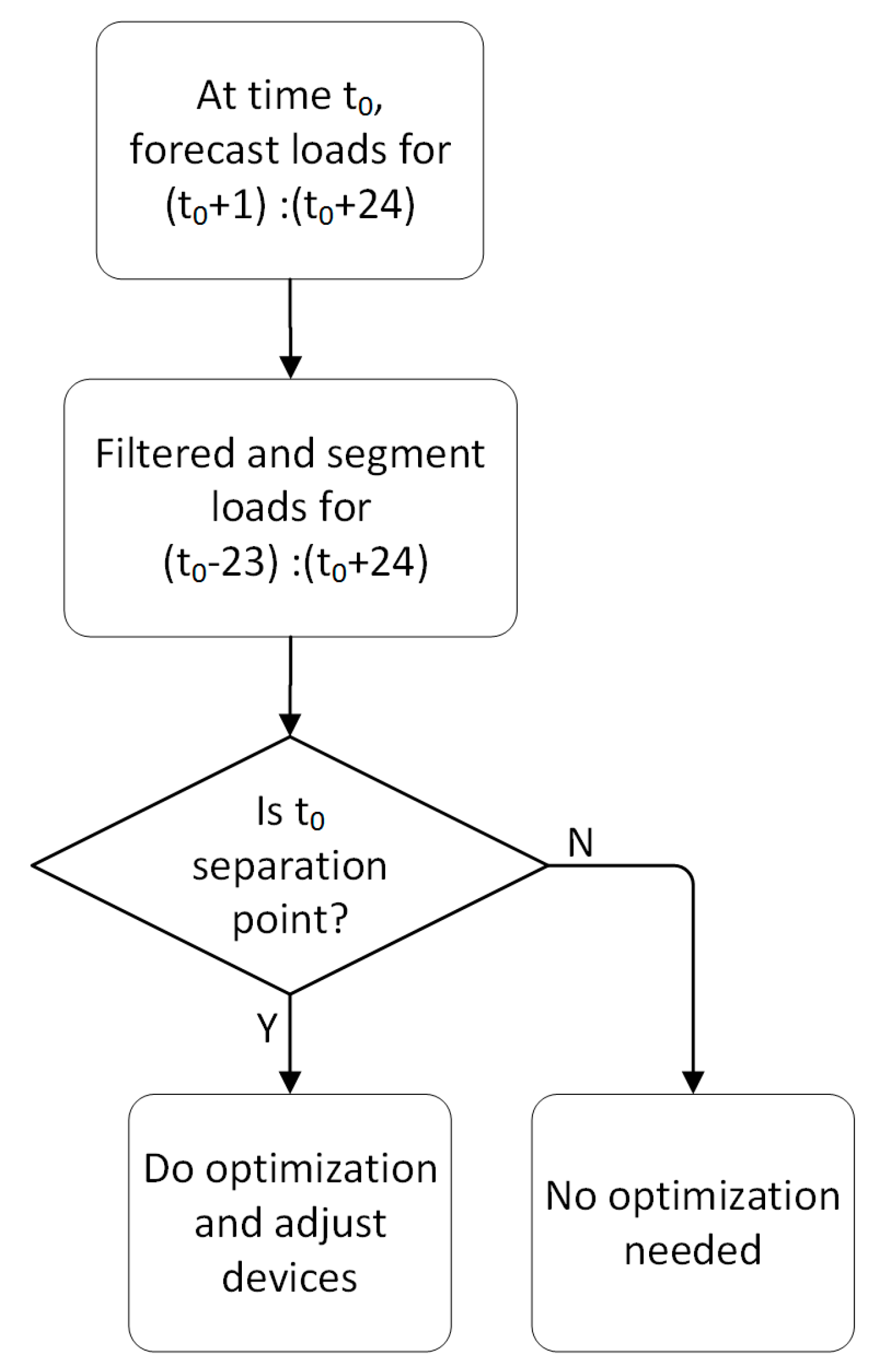
2.4. Optimization in an Online Mode

At each time stamp, hourly forecasts are made for the next 24 h. Due to daily periodic characteristics of load curves, forecasts are made using a multiplicative seasonal auto-regressive integrated moving average model (ARIMA) [19,20]. With consideration of daily periodicity as well as short-term disturbance, ARIMA (0,1,1) with seasonal moving average part MA (24) are applied, i.e., ARIMA (0,1,1) × (0,1,1)₂₄.

$$(1-B)(1-B^{24})L_t=(1-{\theta }_{1}B)(1-{\mathrm{\Theta }}_1{B}^{24}){\epsilon }_t$$

(10)

where, $L_t$ is time series of load, $B$ is backward shift operator, ${\theta }_1$ and ${\mathrm{\Theta }}_1$ are non-seasonal and seasonal moving average coefficients respectively, ${\epsilon }_t$ represents a random component at time $t$. The value of ${\theta }_1$ and ${\mathrm{\Theta }}_1$ can be estimated from history observations using the maximum likelihood method.

The predicted loads are then combined with observations in the past 24 h, and be filtered and segmented using the method aforementioned. Afterward, optimization is conducted if the current time stamp corresponds to a separation point. The optimization is based on average load level for current time segment. Figure 1 presents the flow chart of the online optimization strategy.

3. Case Studies

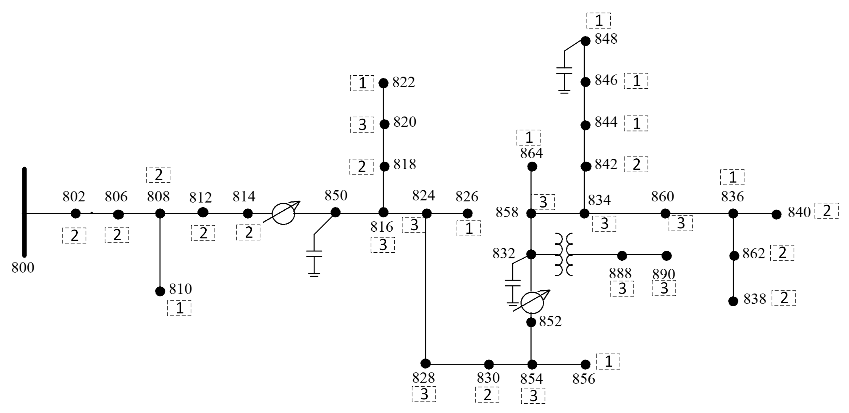
The proposed strategy was verified using a modified IEEE 34-bus test distribution system [21]. As shown in Figure 2, the system has two voltage regulators and three switchable capacitor banks. Each regulator has voltage change range of ±10% and 32 steps, with each step amounting to a 5/8% voltage change. Three 6 × 100 kVar capacitor banks are added to bus 848, 832 and 850. The voltage levels in the distribution system contain 69 kV, 24.9 kV and 4.16 kV.

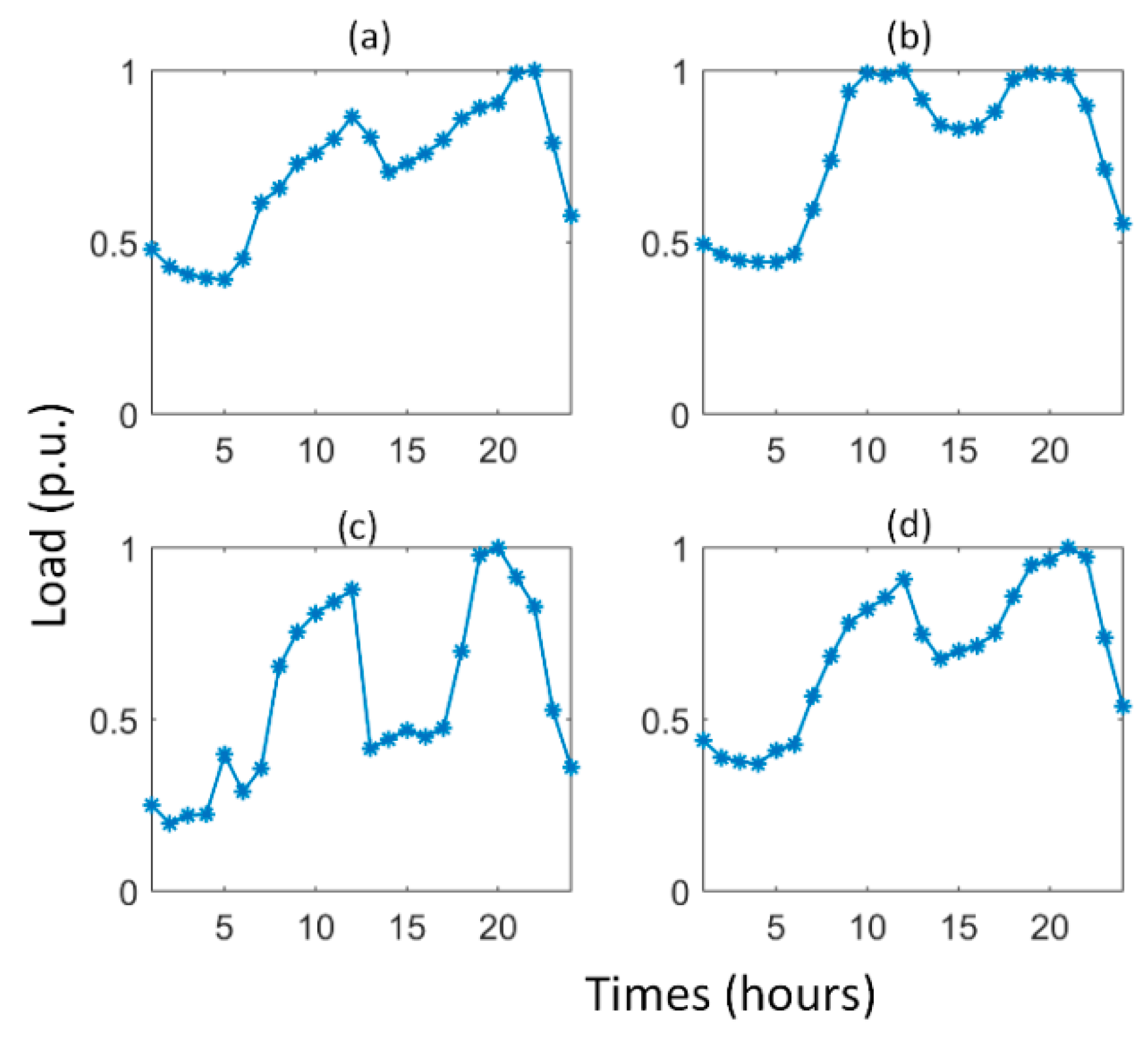
Three daily load curves used in the simulation were extracted from measurements at user side of a 10 kV distribution system. The original 5-min measurements are first aggregated into hourly ones, and the load factor for each hour is afterwards averaged using two-month data [22]. The numbers 1 to 3 in Figure 2 represent the associated load curve at each bus node. Three daily load curve used in the experiment are illustrated in Figure 3. Peak loads occur during the period of 9 am to 11 am as well as 6 pm to 9 pm. Note that the base load values refer to that defined in the original IEEE 34-bus testing system. The integrated load curve is calculated and shown in Figure 3d.

As for optimization method, a genetic algorithm (GA) [23,24], which uses chromosomes instead of real parameter to imitate natural selection process, is an efficient method for the optimization of complex and non-linear problems, thus is carried out to produce optimal reactive power control strategies.

Since the optimization problem here involves objective functions with a number of local extreme points and non-linear constraints, the initial population should be generated with consideration of covering the whole solution space. In this work, the number of members in initial population is set as 50 and point pseudo random number generator is used to generate initial population. Crossover, mutation and selection are then carried out. The involved parameters such as crossover and mutation probabilities, maximal generation number, as well as tolerance level in objective function are obtained using a trial and error scheme. GA is programmed in Matlab platform, and the power flow is calculated using a simulation tool, named the Open Distribution System Simulator (OpenDSS) [25].

3.1. Case Study in an Offline Mode

The proposed strategy is first verified in an offline mode. Four cases using different strategies and filtering methods are applied and compared. Details are shown in

Table 1. Experimental parameters for case 1 to 4.

Case No.	Segmentation Applied	Filtering Method Used in Segmentation	Use Integrated Curve	Number of Segments
Case 1	No	--	--	24
Case 2	Yes	method 1 as in (1)	Yes	6
Case 3	Yes	method 2 as in (2)	Yes	7
Case 4	Yes	method 2 as in (2)	No	9

.

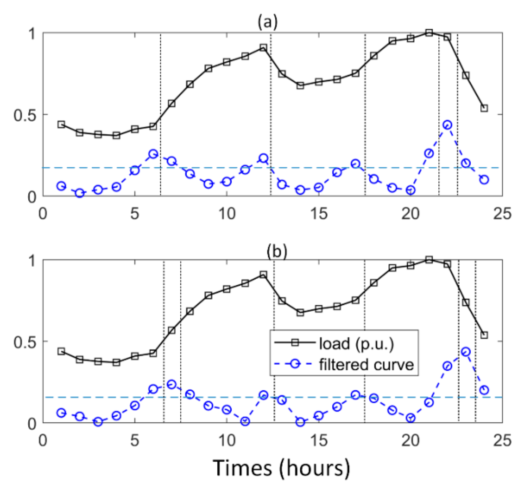
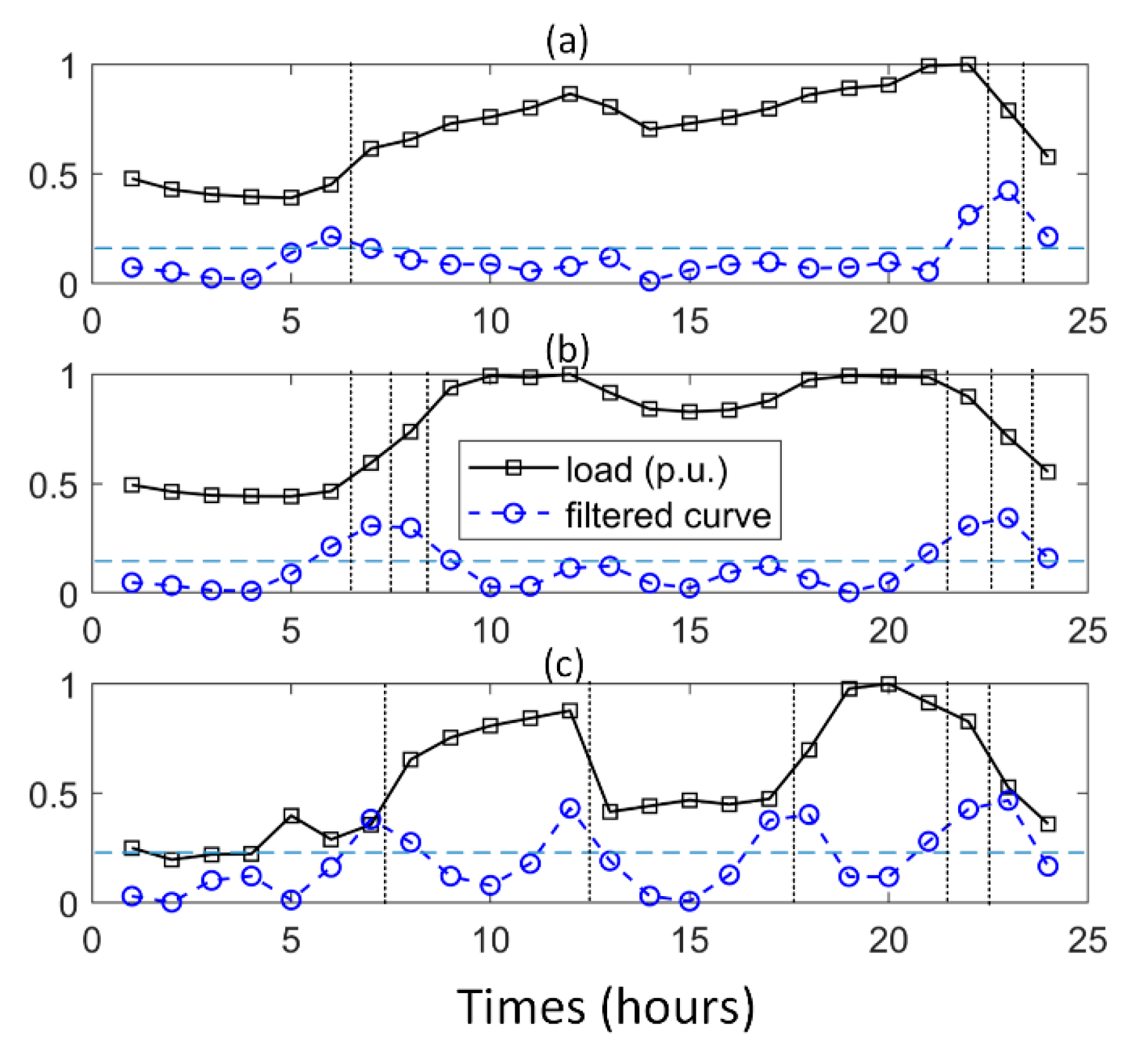
In case 1, no segmentation is applied. In the other three cases, load curve segmentation strategy mentioned in Section 2 is utilized. A filtering signal (blue line shown in Figure 4) is first calculated from load time series using filtering methods 1 or 2, and then thresholded to obtain separation points. Cases 2 and 3 use integrated load curve, the former follows filtering method 1 and the latter uses method 2. Figure 4 and Figure 5 illustrate separation results in cases 2 to 4. Time stamps above the threshold line, i.e., horizontal dashed line, are extracted as separation points. The vertical dashed lines indicate boundaries between segments. There is a slight difference in segmentation results by the two filtering methods, as in Figure 4. Figure 5 shows that case 4 produces more segments than case 2 and 3 because it uses all three load curves independently for segmentation.

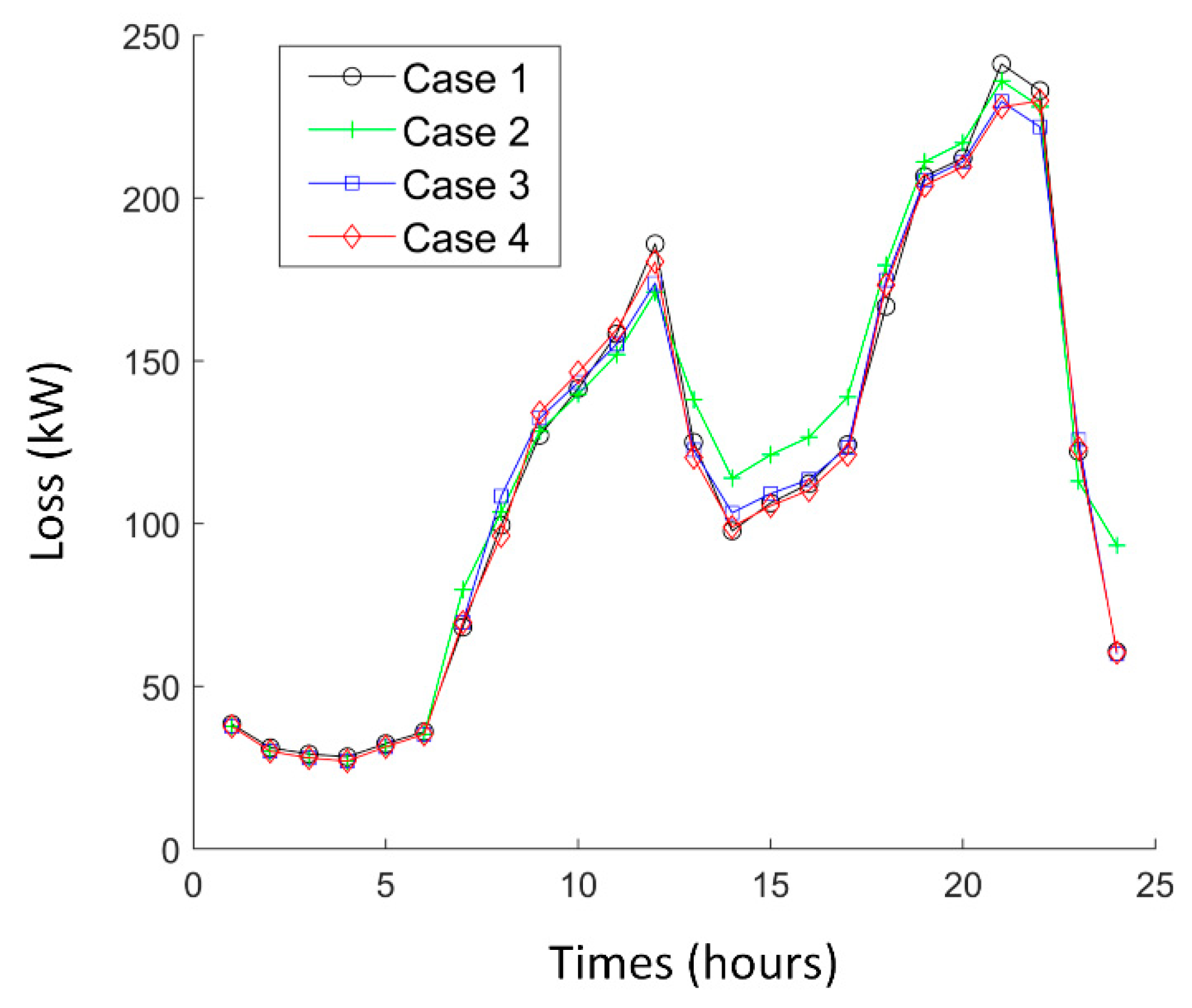
Optimization is afterwards conducted based on the average load in each load segment. As shown in Figure 6, network losses are slightly higher in case 2.

Table 2. Network losses, device adjustment times and time consumed by cases 1 to 4.

Case No.	Total Losses (kWh)	Tap Changes (Times)	Capacitor Changes (Times)	Computation Time (s)
Case 1	2782.9	17	3	2744.99
Case 2	2879.0	8	6	602.38
Case 3	2771.9	7	2	638.28
Case 4	2759.1	10	3	881.72

also shows that case 2 produces the highest losses while case 4 gives the lowest.

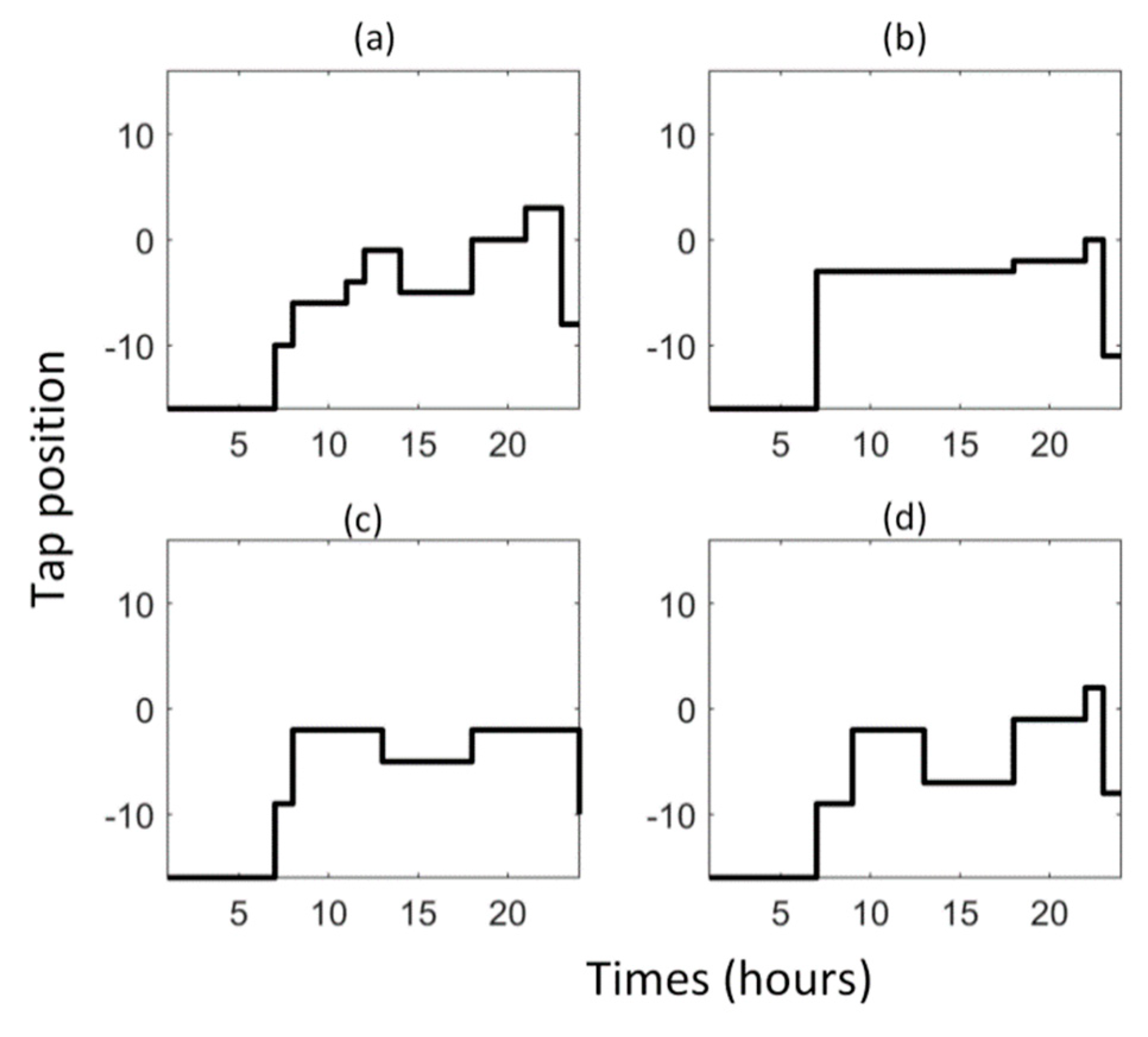
The tap changes of one regulator in four cases are illustrated in Figure 7. It is clear that case 1 presents most frequent tap changes, and cases 2 and 3 the least. The tap changing times have positive correlation with the segment number involved.

Table 2 also shows that case 1 consumed three times of computation time compared with other cases. Lowest network loss presented in case 4 is at the sacrifice of adjusting times. Cases 2 and 3 are comparable with regard to time efficiency while case 3 presented better performance on network losses, indicating the merits of filtering method 2.

It could be concluded in this part that the segmentation strategies based on integrated load curve highly improved computational efficiency and at the same time gave satisfactory optimization performance. In addition, filtering method 2 is slightly better than method 1 in terms of obtained network losses.

3.2. Case Study in an Online Mode

Previous offline case studies verified the merits of the proposed strategy based on integrated load curve and filtering method 2. An online case study is thus conducted here using filtering method 2 and integrated load curve.

Time series of three types of loads, as in offline case studies, are also used here. For comparison, case 5 optimizes at each time point using only current load measurement without consideration of load curve prediction or segmentation. In case 6, the proposed strategy is applied, as shown in

Table 3. Experimental parameters for cases 5 and 6.

Case No.	Using Predicted Load Series	Segmentation Applied	Filtering Method Used	Use Integrated Curve	Number of Segments
Case 5	No	No	--	--	24
Case 6	Yes	Yes	method 2 as in (2)	Yes	8

.

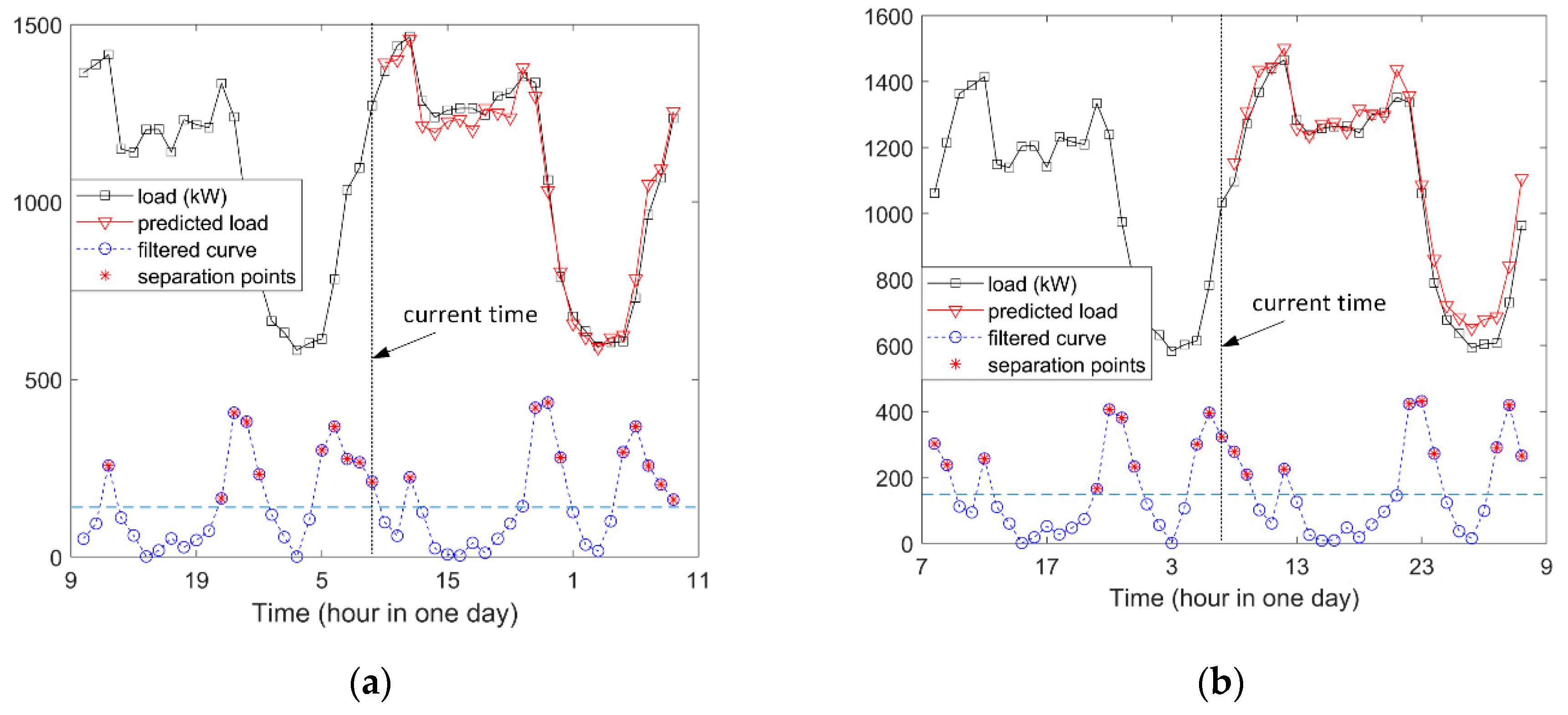
In case 6, for each hour in a daily cycle, hourly load forecasts are made for the next day and for each type of load. The forecasts and previous observations form a 48-h load curve, which is then filtered using method 2 in (2) and segmented. If the current time is considered as a separation point, then optimization is applied based on averaged load level in an associated segment. In Figure 8a, black line indicates load curve observed, the red line predicted ones. Filtering is conducted for 48-h time series, and then the current time, i.e., 9 am, is detected as a separation point. Thus, optimization is conducted based on average load during current segment, i.e., time period from 9 am to 12 am. In Figure 8b, optimization should be based on load level at current time, i.e., 7 am, because it is detected as a separation point.

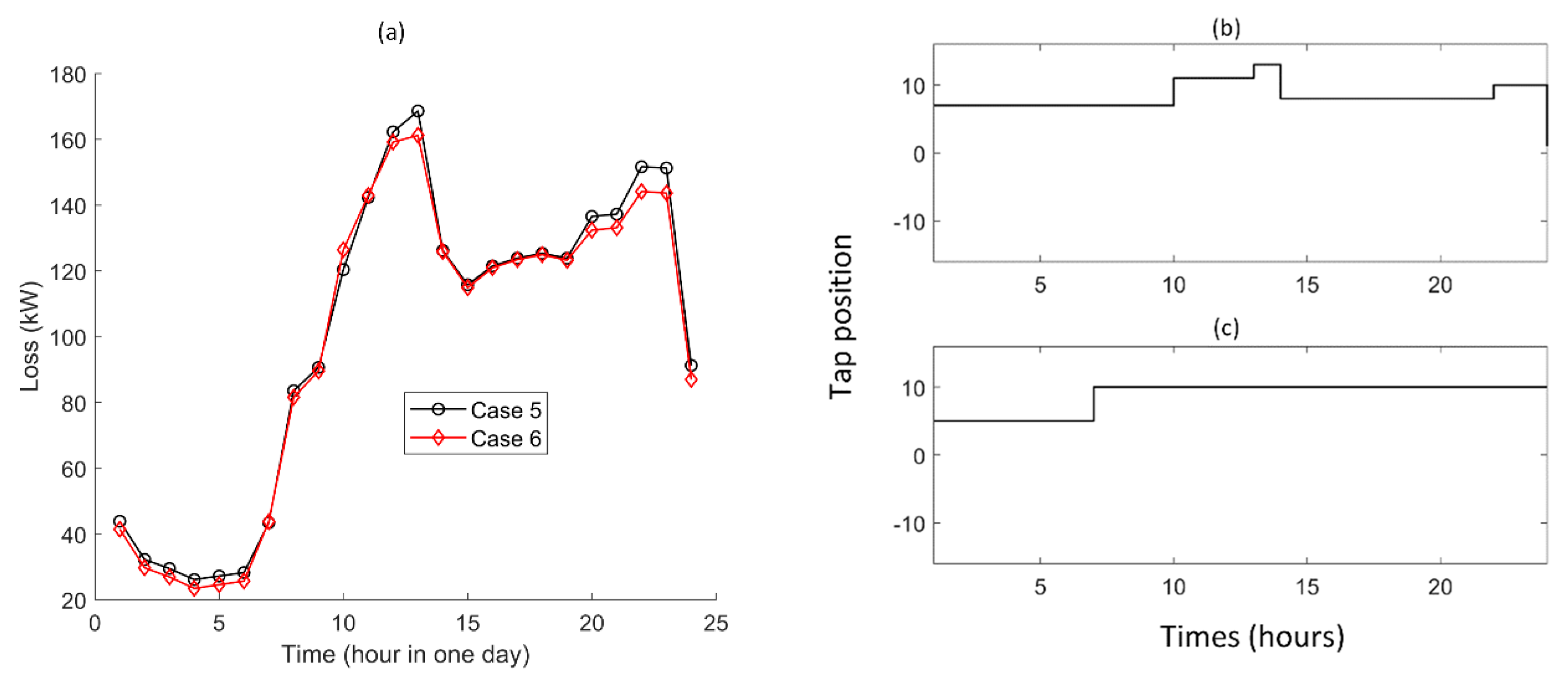
Figure 9a shows comparisons of two cases w.r.t. network losses. It is found that case 6 presents relatively lower losses. Figure 9b,c illustrate that tap changes produced by case 6 are less than that in case 5. Again, the tap changing times have positive correlation with the segment number involved.

Table 4. Network losses, device adjustment times and time consumed by cases 5 and 6.

Case No.	Total Losses (kWh)	Tap Changes (Times)	Capacitor Changes (Times)	Computation Time (s)
Case 5	2403.1	8	3	1774.08
Case 6	2350.1	6	1	818.81

presents comparisons in terms of device adjusting times and network losses. Case 5 produces eight tap changing times while case 6 only output six. Network losses in case 5 are slightly less than in case 6. The computation time consumed by case 5 is two times more than that in case 6. This evidence that the proposed strategy gave a satisfactory performance in both optimization results as well as computational efficiency.

4. Discussion

Through offline and online case studies over a modified IEEE 34-bus test distribution system, the experimental results gave evidence that,

(1).

Reactive power optimization based on load curve prediction and segmentation is able to reduce reactive power compensation device adjustment times effectively, reduce network losses during a duty cycle to some extent, and at the same time improve computational efficiency;

(2).

Compared with using individual load curve for segmentation, using integrated load curve is adequate to produce better optimization performance w.r.t. device adjustment times and to reduce computational burden, at the sacrifice of total network losses to some extent;

(3).

The optimal adjustment times of tap changers and capacitors have positive correlation with the number of load curve segments;

(4).

When doing load curve segmentation, filtering method 2 is superior to filtering method 1 in terms of optimization performance.

5. Conclusions

In distribution systems, variations of loads bring serious challenges to system operation. Moreover, the temporal variations of different types of loads are not the same, thus it is essential to conduct dynamic reactive power optimization for a certain time period instead of one time stamp. This paper proposed a strategy which segments the predicted integrated load curve first, and then conducts optimization using GA with adjustment times of reactive compensation devices as one objective. Through case studies for a modified IEEE 34-bus system and three load curves extracted from field measurements, experimental results evidenced that, compared with optimization without load curve segmentation, the proposed strategy is able to produce satisfactory optimization results in terms of network losses and device adjustment times; additionally, it is able to reduce computation burden effectively at the same time. In the future, efforts will be made to improveme sequence power flow calculation, which is an important procedure involved in dynamic reactive power optimization.