Super-Resolution Reconstruction Algorithm for Infrared Image with Double Regular Items Based on Sub-Pixel Convolution

Abstract
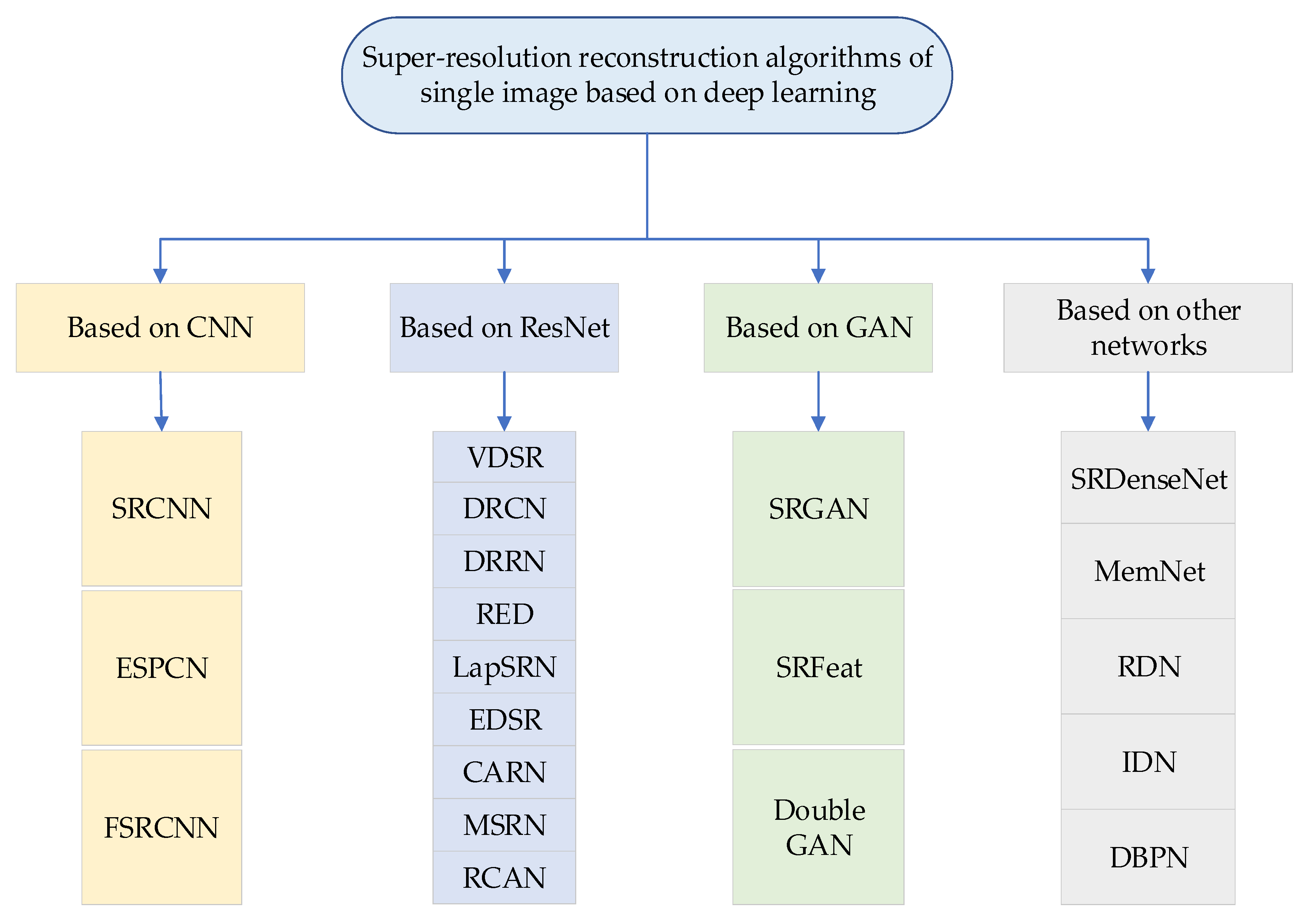
1. Introduction
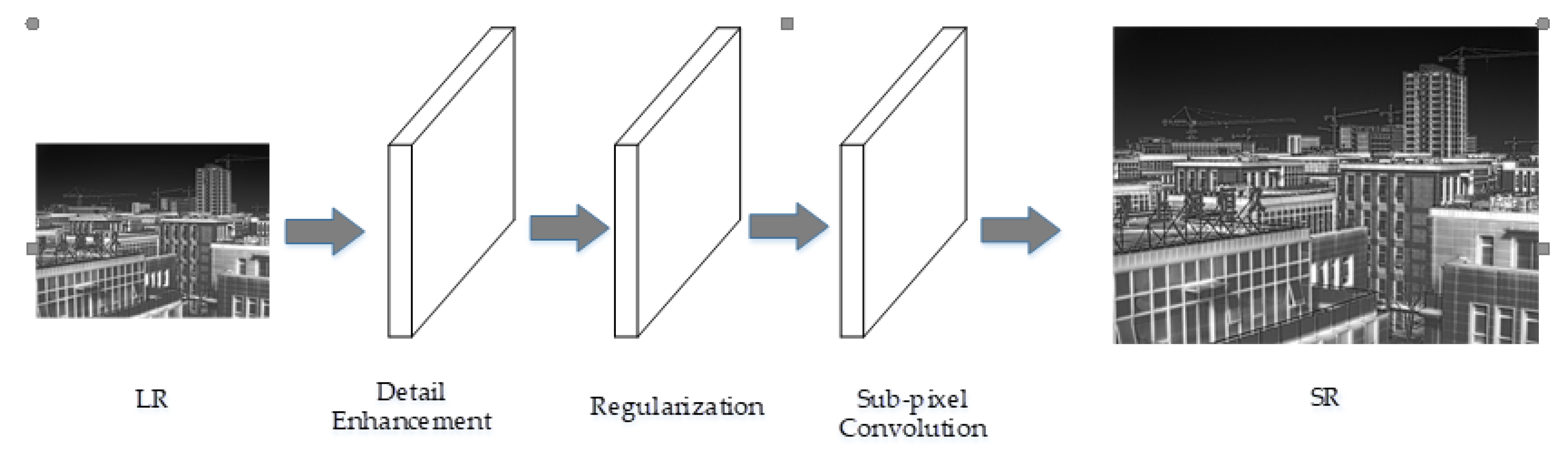
2. Methods
2.1. Multi-Scale Detail Enhancement
2.2. Adaptive Regularization Algorithm Based on Maximum a Posteriori Estimation
2.2.1. Related Algorithm
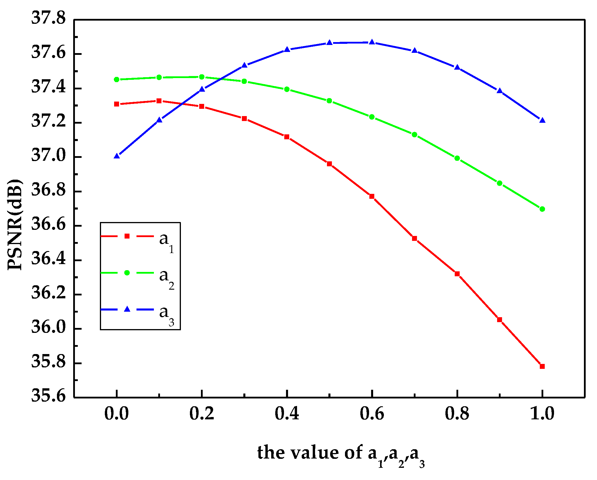
2.2.2. Improvement of Regularization
2.3. Combining Regularization with Sub-Pixel Convolution
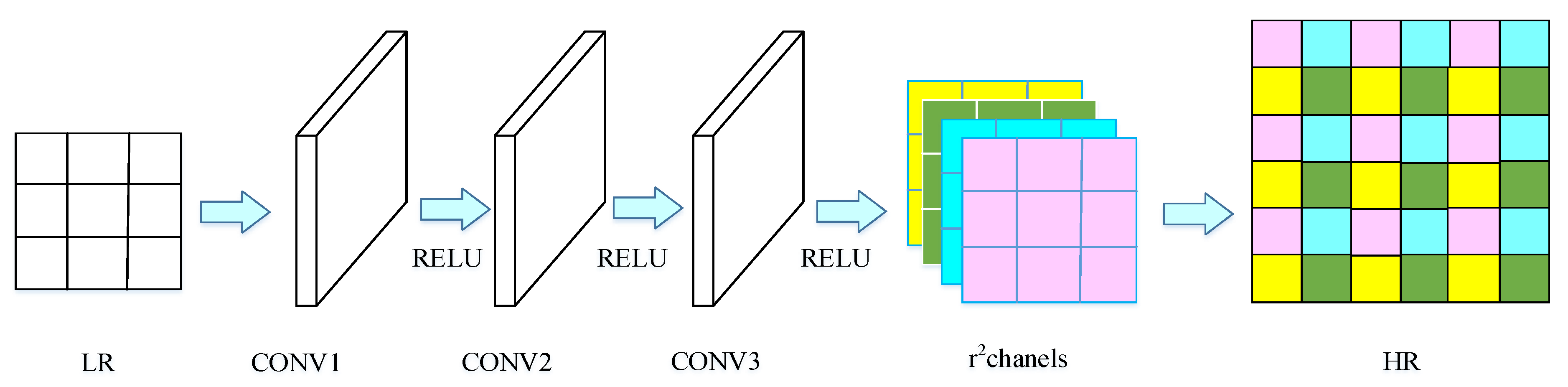
2.3.1. Basic Theory of Sub-Pixel Convolution
2.3.2. Combining Regularization with Sub-Pixel Convolution
| Algorithm1 MPSR algorithm |
| 1: Input: Low resolution image X, up-sampling factor s. |
| 2: Step 1: Multi-scale detail enhancement for X. |
| 3: Step 2: Initial image reconstruction using regularized objective function. |
| 4: (1) Parameter initialization: |
| 5: , , , |
| 6: (2) Reconstruction from objective function: |
| 7: |
| 8: (3) Adjust adaptive parameters: |
| 9: |
| 10: |
| 11: (4) |
| 12: (5) If : |
| 13: Yes, Go back to 2); |
| 14: No, output, |
| 15: Step 3: Image magnification by sub-pixel convolution |
| 16: (1) Using convolution layers to extract image features |
| 17: (2) Generation of high-resolution image by sub-pixel convolution |
| 18: Output: High-resolution image |
3. Experiments and Results
3.1. Complexity Analysis
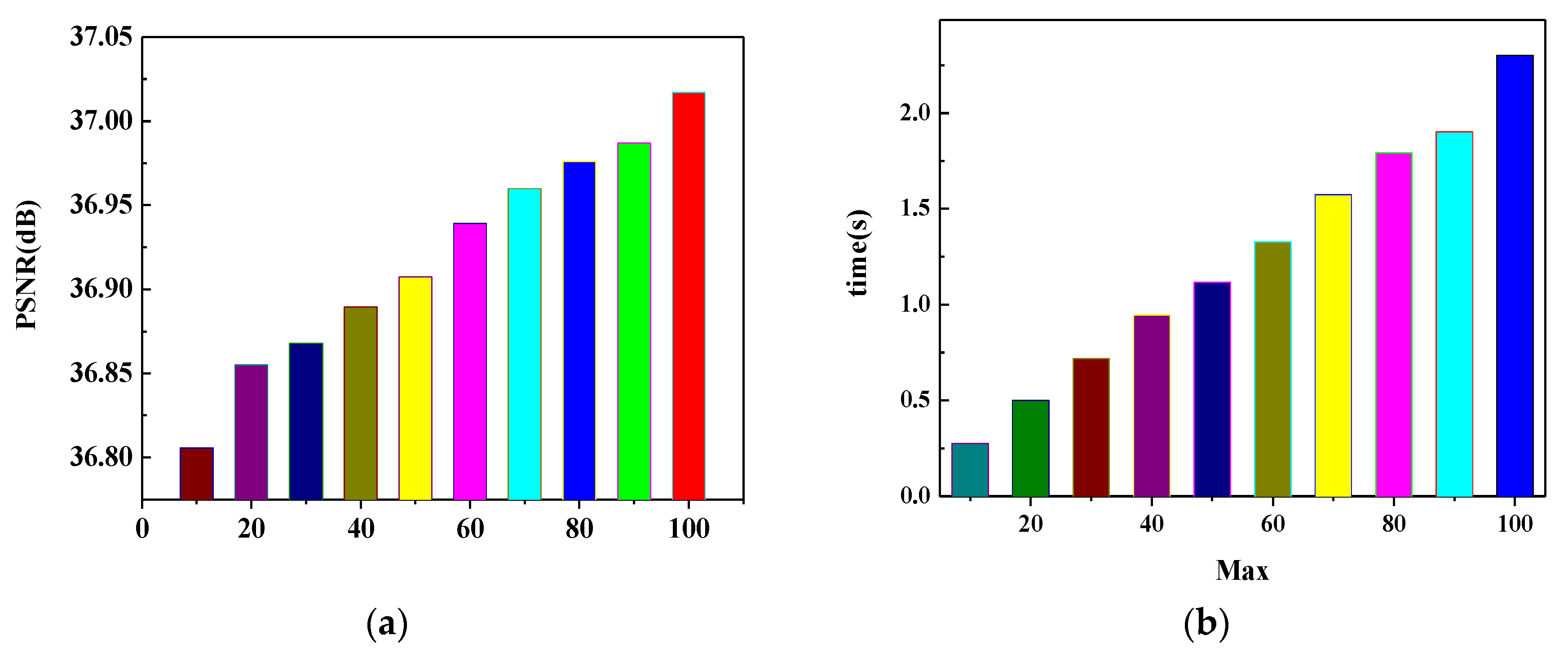
3.2. Experimental Environment and Parameters Setting
3.3. Image Quality Metric Parameters
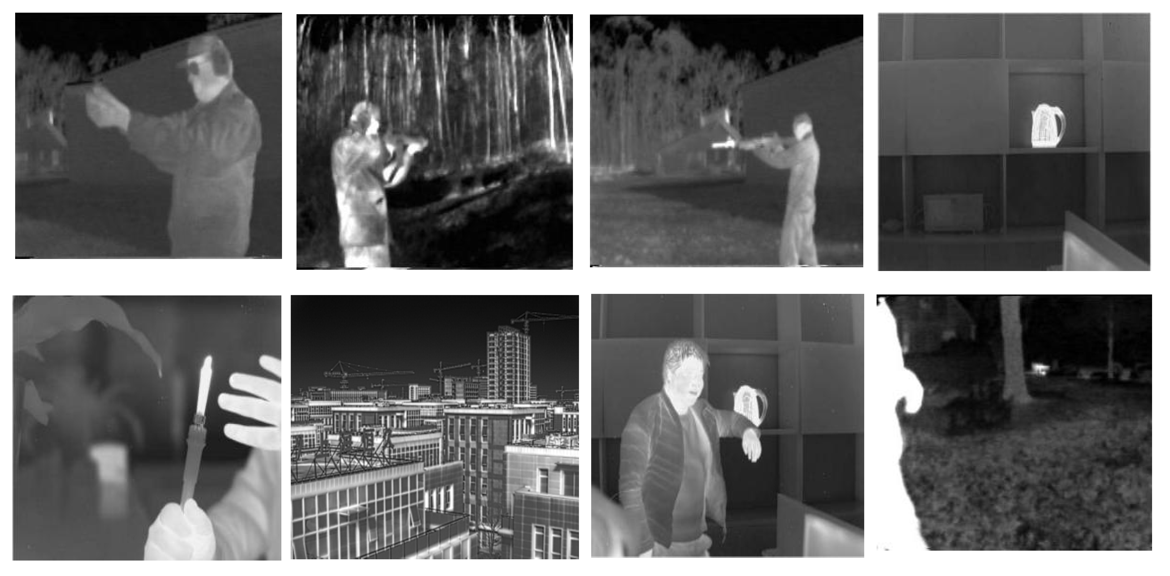
3.4. Experimental Results
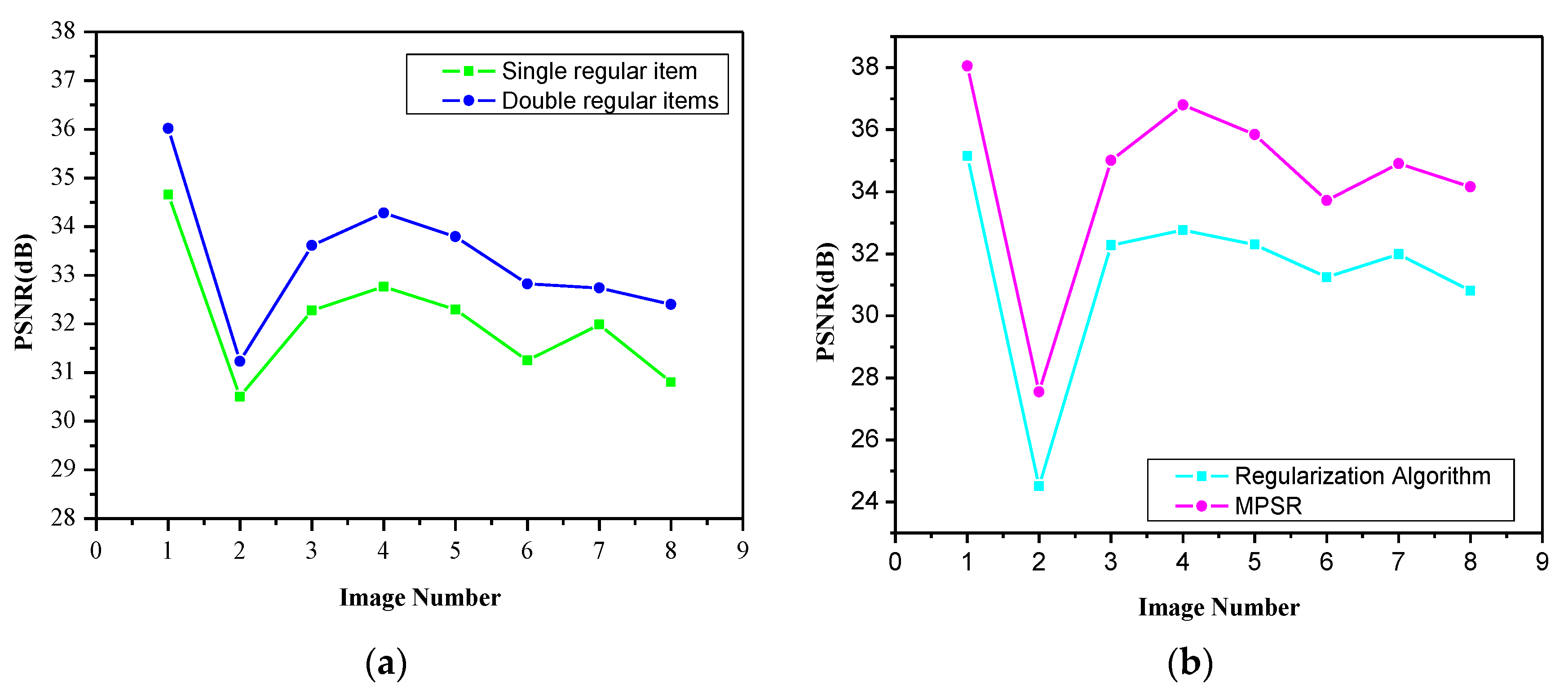
3.4.1. Experiment on the Effectiveness of Algorithm Improvements
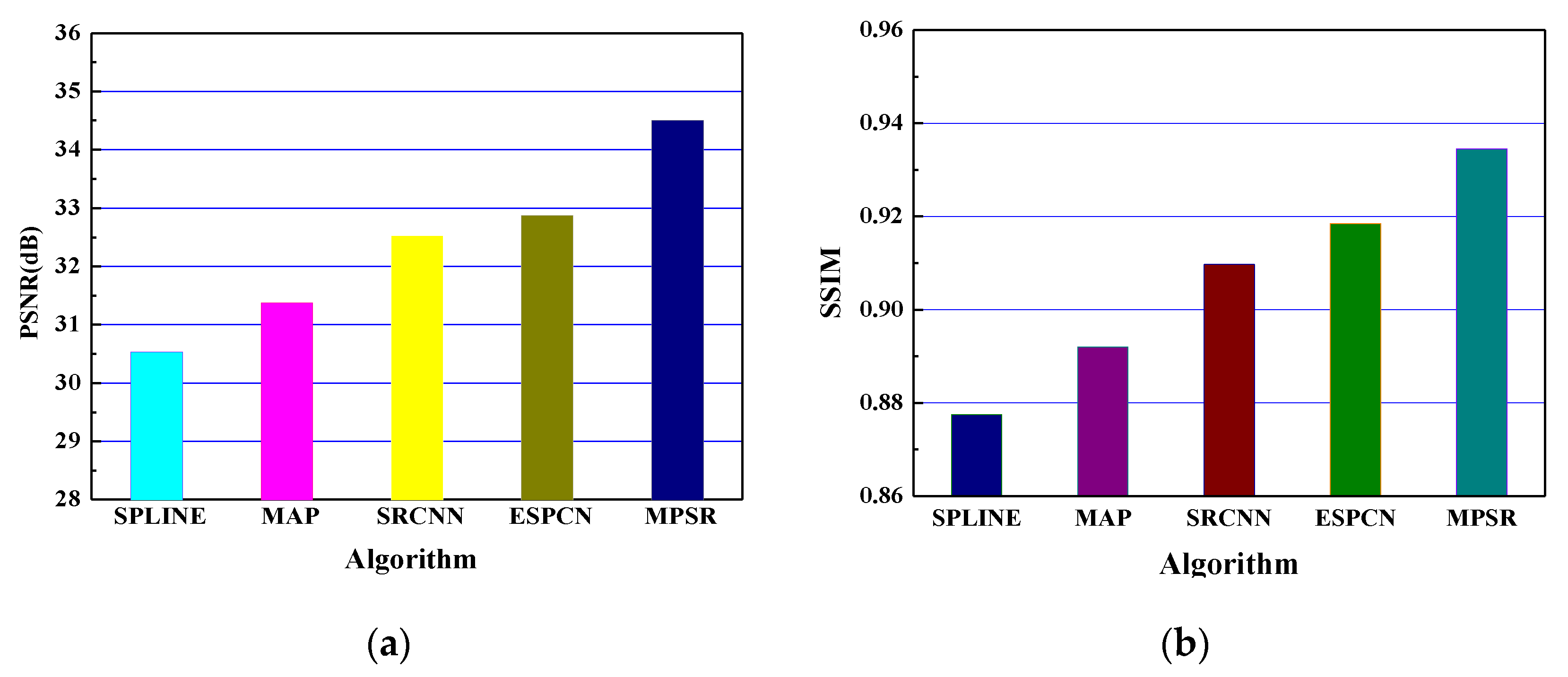
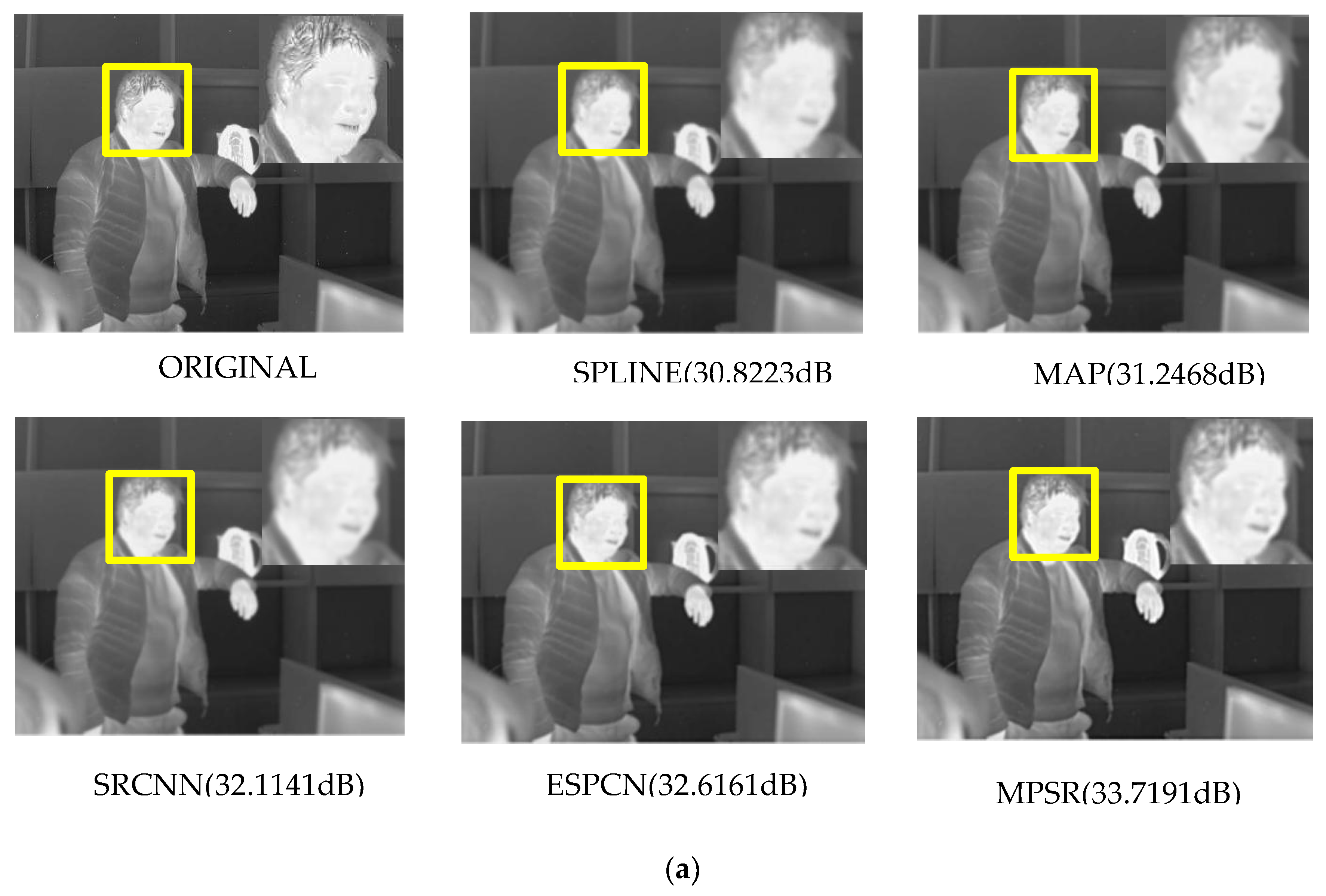
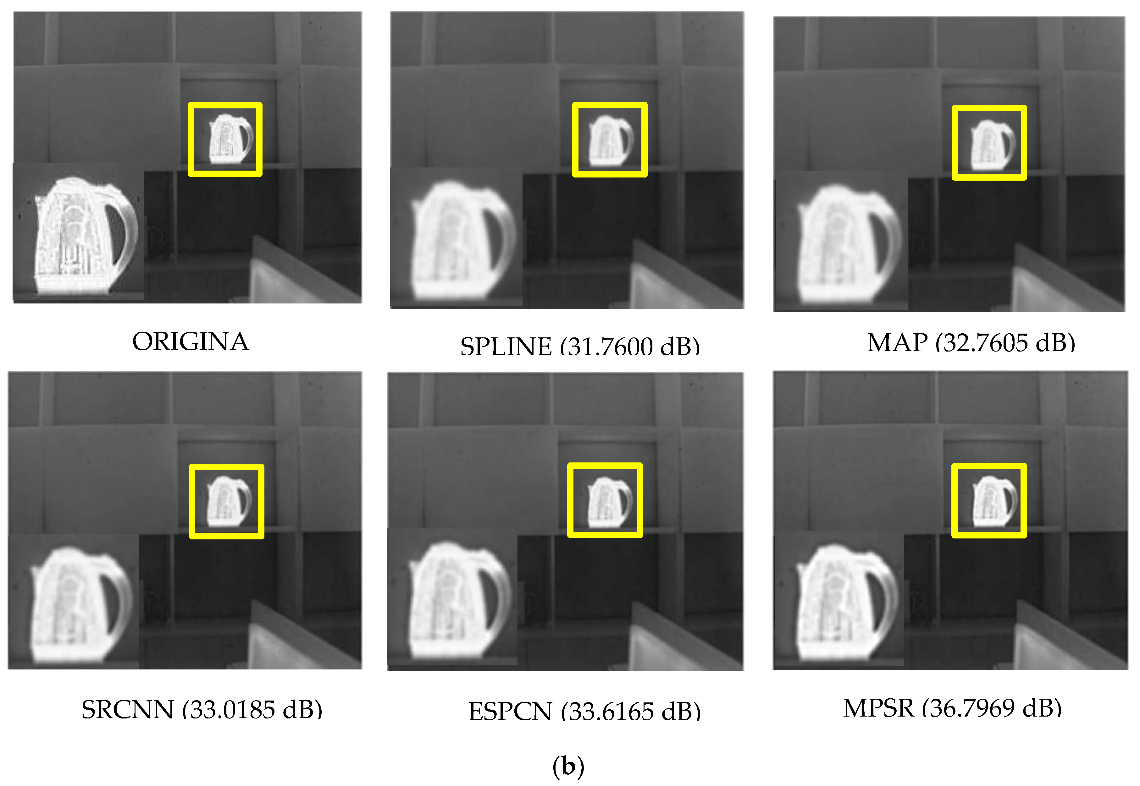
3.4.2. Comparison of Different Algorithms
4. Conclusions
Author Contributions
Funding
Acknowledgments
Conflicts of Interest
References
- Liu, D.; Wang, Z.; Wen, B.; Yang, J.; Han, W.; Huang, T.S. Robust single image super-resolution via deep networks with sparse prior. IEEE Trans. Lynage Process. 2016, 25, 3194–3207. [Google Scholar] [CrossRef]
- Thornton, M.W.; Atkinson, P.M.; Holland, D.A. Sub-pixel mapping of rural land cover objects from fine spatial resolution satellite sensor imagery using super-resolution pixel-swapping. Int. J. Remote Sens. 2006, 27, 473–491. [Google Scholar] [CrossRef]
- Fan, Y.; Yu, J.; Huang, T.S. Wide-activated Deep Residual Networks based Restoration for BPG-compressed Images. In Proceedings of the IEEE Conference on Computer Vision and Pattern Recognition (CVPR) Workshops, Salt Palace Convention Cetner, Salt Lake City, UT, USA, 18–22 June 2018. [Google Scholar]
- Yu, J.; Lin, Z.; Yang, J.; Shen, X.; Lu, X.; Huang, T.S. Free-Form Image Inpainting with Gated Convolution. arXiv 2018, arXiv:1806.03589. [Google Scholar]
- Yu, J.; Lin, Z.; Yang, J.; Shen, X.; Lu, X.; Huang, T.S. Generative Image Inpainting with Contextual Attention. arXiv 2018, arXiv:1801.07892. [Google Scholar]
- Dong, C.; Loy, C.C.; He, K.; Tang, X. Learning a deep convolutional network for image super-resolution. In Proceedings of the European Conference on Computer Vision, Zurich, Switzerland, 6–12 September 2014; Springer: Berlin/Heidelberg, Germany, 2014; pp. 184–199. [Google Scholar]
- Dong, C.; Loy, C.C.; Tang, X. Accelerating the super-resolution convolutional neural network. In Proceedings of the European Conference on Computer Vision, Amsterdam, The Netherlands, 11–14 October 2016; Springer: Berlin/Heidelberg, Germany, 2016; pp. 391–407. [Google Scholar]
- Shi, W.; Caballero, J.; Huszar, F.; Totz, J.; Andrew, A.P.; Bishop, R.; Rueckert, D.; Wang, Z. Real-time single image and video super-resolution using an efficient sub-pixel convolutional neural network. In Proceedings of the IEEE Conference ore Computer Vision and Pattern Recognition, Las Vegas, NV, USA, 26 June–1 July 2016; pp. 1874–1883. [Google Scholar]
- Mao, X.J.; Shen, C.; Yang, Y.B. Image restoration us-ing very deep convolutional encoder-decoder networks withsymmetric skip connections. In Proceedings of the Interna-Tional Conference on Neural Information Processing Sys-Tems, NIPS, Barcelona, Spain, 5–10 December 2016; pp. 2802–2810. [Google Scholar]
- Ahn, N.; Kang, B.; Sohn, K.A. Fast, accurate, and lightweightsuper-resolution with cascading residual network. In Proceedings of the 2018 ECCV European Conference on Computer Vision, Munich, Germany, 8–14 September 2018; Springer: Berlin/Heidelberg, Germany, 2018; pp. 256–272. [Google Scholar]
- Ledig, C.; Wang, Z.; Shi, W. Photo-realistic single image super-resolution using a generative adversarial network. In Proceedings of the IEEE Conference on Computer Vision and Pat-Tern Recognition, CVPR, Honolulu, HI, USA, 21–26 July 2017; pp. 105–114. [Google Scholar]
- Park, S.J.; Son, H.; Cho, S.H. SRFeat: Single image super-resolution with feature discrimination. In Proceedings of the 2018 ECCV European Conference on Computer Vision, Munich, Germany, 8–14 September 2018; Springer: Berlin/Heidelberg, Germany, 2018; pp. 455–471. [Google Scholar]
- Zhang, Y.L.; Tian, Y.; Kong, Y.; Zhong, B.; Fu, Y. Residual densenetwork for image super-resolution. In Proceedings of the IEEE Conference on Computer Vision and Pattern Recognition, CVPR, Salt Lake City, UT, USA, 18–22 June 2018; pp. 2472–2481. [Google Scholar]
- Hui, Z.; Wang, X.; Gao, X. Fast and accurate single imagesuper-resolution via information distillation network. In Proceedings of the IEEE Conference on Computer Vision and Pattern Recognition, CVPR, Salt Lake City, UT, USA, 18–22 June 2018; pp. 723–731. [Google Scholar]
- Haris, M.; Shakhnarovich, G.; Ukita, N. Deep back-projectionnetworks for super-resolution. In Proceedings of the IEEE Conference on Computer Vision and Pattern Recognition, CVPR, Salt Lake City, UT, USA, 18–22 June 2018; pp. 1664–1673. [Google Scholar]
- Zhou, F.; Yang, W.; Liao, Q. Interpolation-based image super-resolution using multisurface fifitting. IEEE Trans. Image Process. 2012, 21, 3312–3318. [Google Scholar] [CrossRef] [PubMed]
- Wang, E.; Jiang, P.; Hou, X.; Zhu, Y.; Peng, L. Infrared Stripe Correction Algorithm Based on Wavelet Analysis and Gradient Equalization. Appl. Sci. 2019, 9, 1993. [Google Scholar] [CrossRef]


| Complexity Related Items | SRCNN | MPSR |
|---|---|---|
| Conv1 | (64, 9, 1) | (64, 5, 1) |
| Conv2 | (32, 5, 64) | (64, 3, 64) |
| Conv3 | (1, 5, 32) | (64, 3, 32) |
| Conv4 | None | (4, 3, 32) |
| Input image | ||
| Number of parameters | 57,184 | 58,048 |
| Complexity | 3.9 | 1 |
| Project | Environment/Version |
|---|---|
| Operating system | ubuntu |
| CPU | i7-8700k |
| Memory | 32GB |
| GPU | GTX1080ti |
| Framework | pytorch |
| Python IDE | pycharm |
| Metric Parameters | Number | Image Pixel | SPLINE | MAP | SRCNN | ESPCN | MPSR |
|---|---|---|---|---|---|---|---|
| PSNR (dB) | 1 | 320 * 240 | 34.0800 | 35.1562 | 36.9908 | 37.0787 | 38.0546 |
| 2 | 320 * 240 | 23.6019 | 24.5066 | 25.9310 | 25.9588 | 27.5505 | |
| 3 | 320 * 240 | 31.3120 | 32.2794 | 33.2204 | 33.8099 | 35.0086 | |
| 4 | 320 * 240 | 31.7600 | 32.7605 | 33.0185 | 33.6165 | 36.7969 | |
| 5 | 320 * 240 | 31.8201 | 32.2924 | 33.3726 | 33.6970 | 35.8422 | |
| 6 | 320 * 240 | 30.8223 | 31.2468 | 32.1141 | 32.6161 | 33.7191 | |
| 7 | 320 * 240 | 31.0702 | 31.9873 | 33.3658 | 33.7443 | 34.9114 | |
| 8 | 320 * 240 | 29.8001 | 30.8034 | 32.1989 | 32.5128 | 34.1559 |
| Metric Parameters | Number | Image Pixel | SPLINE | MAP | SRCNN | ESPCN | MPSR |
|---|---|---|---|---|---|---|---|
| SSIM | 1 | 320 * 240 | 0.9113 | 0.9215 | 0.9398 | 0.9429 | 0.9516 |
| 2 | 320 * 240 | 0.7518 | 0.7875 | 0.8315 | 0.8457 | 0.8804 | |
| 3 | 320 * 240 | 0.8779 | 0.8925 | 0.9023 | 0.9194 | 0.9365 | |
| 4 | 320 * 240 | 0.9594 | 0.9617 | 0.9645 | 0.9690 | 0.9736 | |
| 5 | 320 * 240 | 0.9593 | 0.9625 | 0.9659 | 0.9678 | 0.9702 | |
| 6 | 320 * 240 | 0.9175 | 0.9223 | 0.9290 | 0.9360 | 0.9436 | |
| 7 | 320 * 240 | 0.8099 | 0.8340 | 0.8661 | 0.8782 | 0.9059 | |
| 8 | 320 * 240 | 0.8334 | 0.8542 | 0.8784 | 0.8889 | 0.9144 |
© 2020 by the authors. Licensee MDPI, Basel, Switzerland. This article is an open access article distributed under the terms and conditions of the Creative Commons Attribution (CC BY) license (http://creativecommons.org/licenses/by/4.0/).
Share and Cite
Yu, L.; Zhang, X.; Chu, Y. Super-Resolution Reconstruction Algorithm for Infrared Image with Double Regular Items Based on Sub-Pixel Convolution. Appl. Sci. 2020, 10, 1109. https://doi.org/10.3390/app10031109
Yu L, Zhang X, Chu Y. Super-Resolution Reconstruction Algorithm for Infrared Image with Double Regular Items Based on Sub-Pixel Convolution. Applied Sciences. 2020; 10(3):1109. https://doi.org/10.3390/app10031109
Chicago/Turabian StyleYu, Lei, Xuewei Zhang, and Yan Chu. 2020. "Super-Resolution Reconstruction Algorithm for Infrared Image with Double Regular Items Based on Sub-Pixel Convolution" Applied Sciences 10, no. 3: 1109. https://doi.org/10.3390/app10031109
APA StyleYu, L., Zhang, X., & Chu, Y. (2020). Super-Resolution Reconstruction Algorithm for Infrared Image with Double Regular Items Based on Sub-Pixel Convolution. Applied Sciences, 10(3), 1109. https://doi.org/10.3390/app10031109