Measurements of Entropic Uncertainty Relations in Neutron Optics


Abstract
1. Introduction
2. Theory
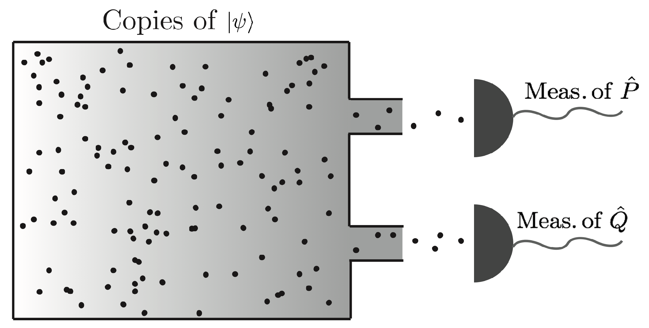
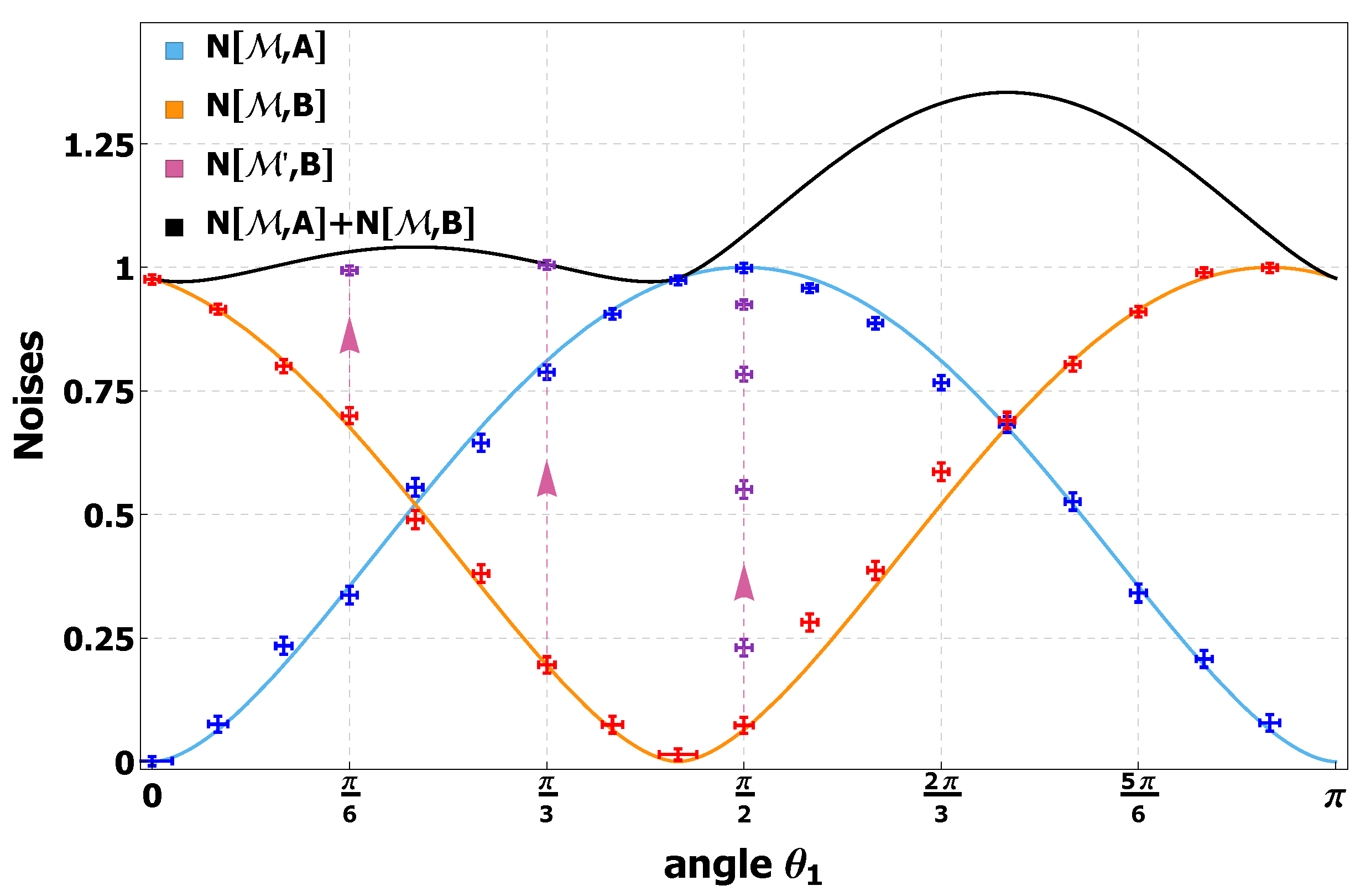
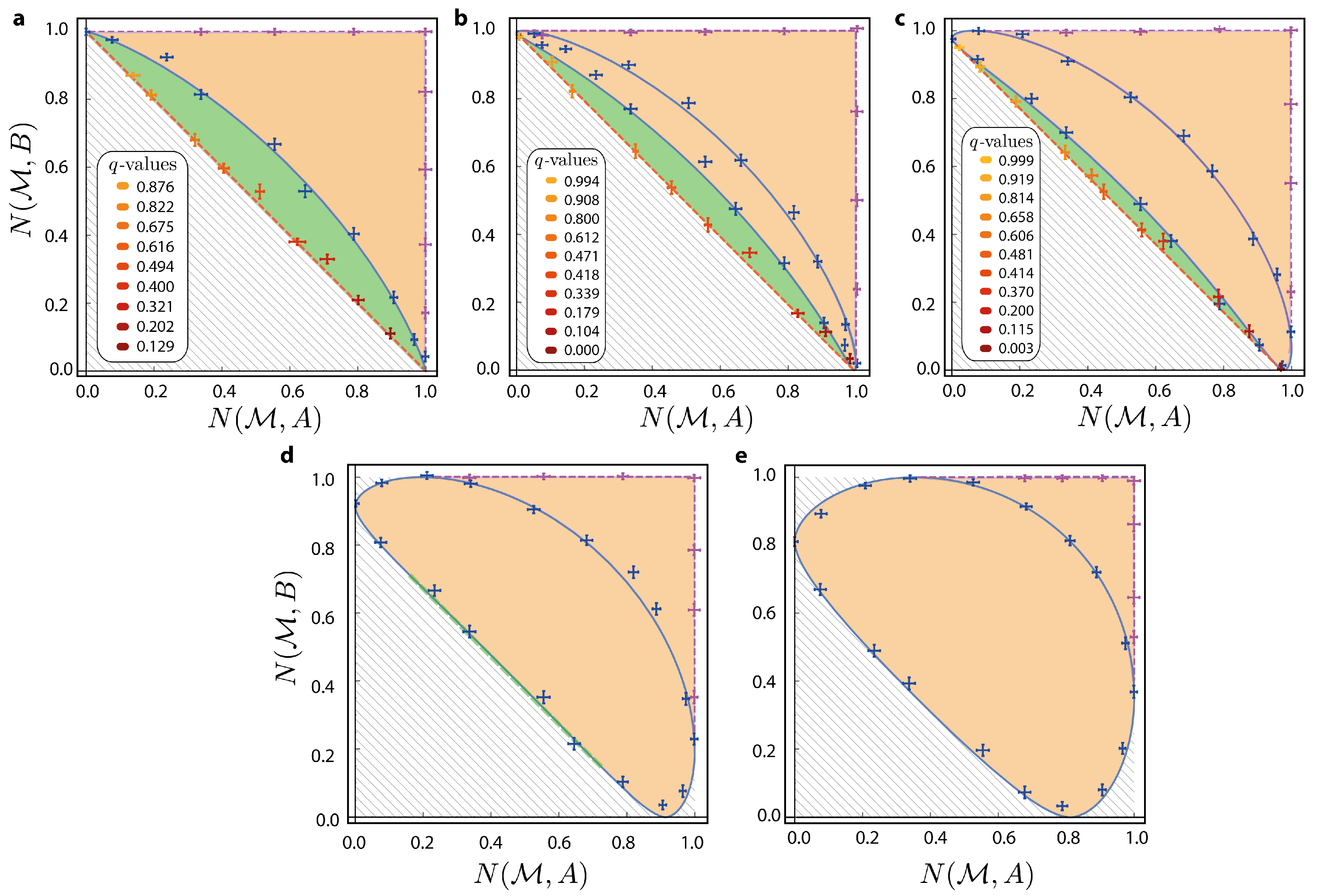
- Noise–noise uncertainty relationThis tradeoff expresses the inability for the device to jointly discriminate the eigenstates and to arbitrary precision.
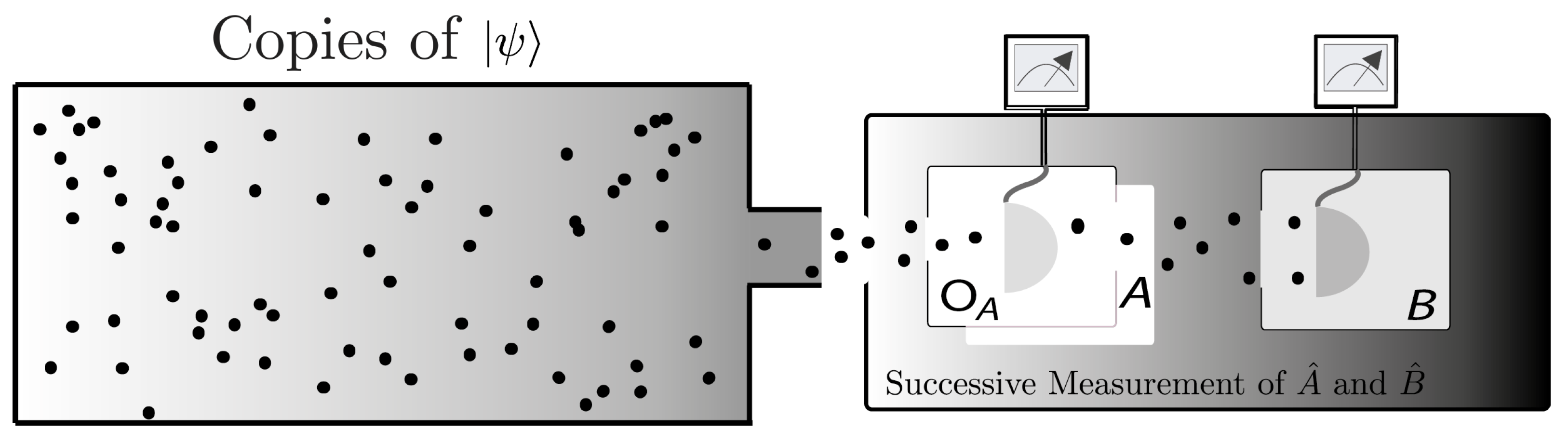
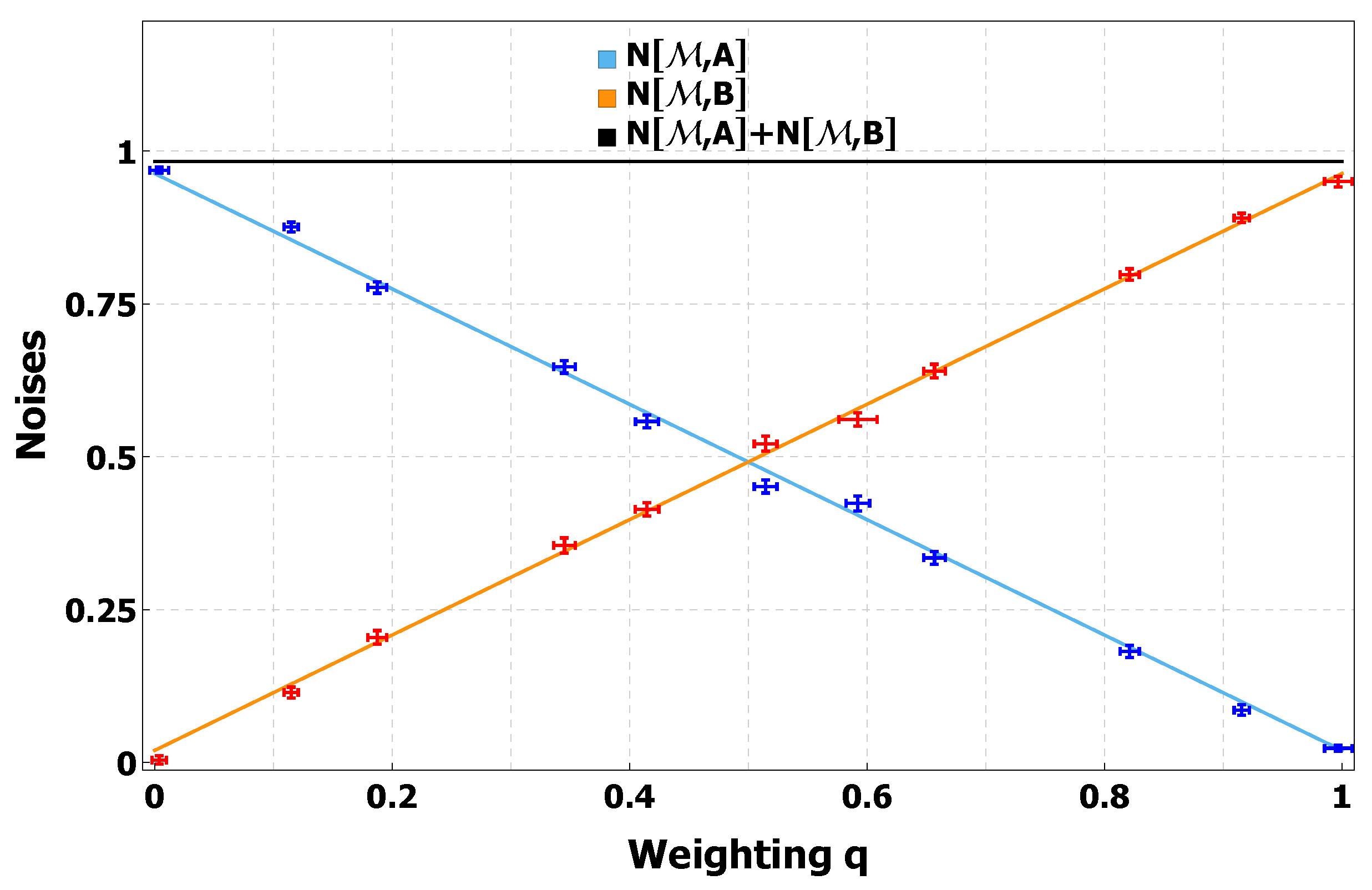
- Noise–disturbance uncertainty relationThis inequality implies that the measurement apparatus cannot be noise and disturbance-free for both eigenstates of the non-commuting operators A and B.
Entropic Measurement Uncertainty Relation for Qubits
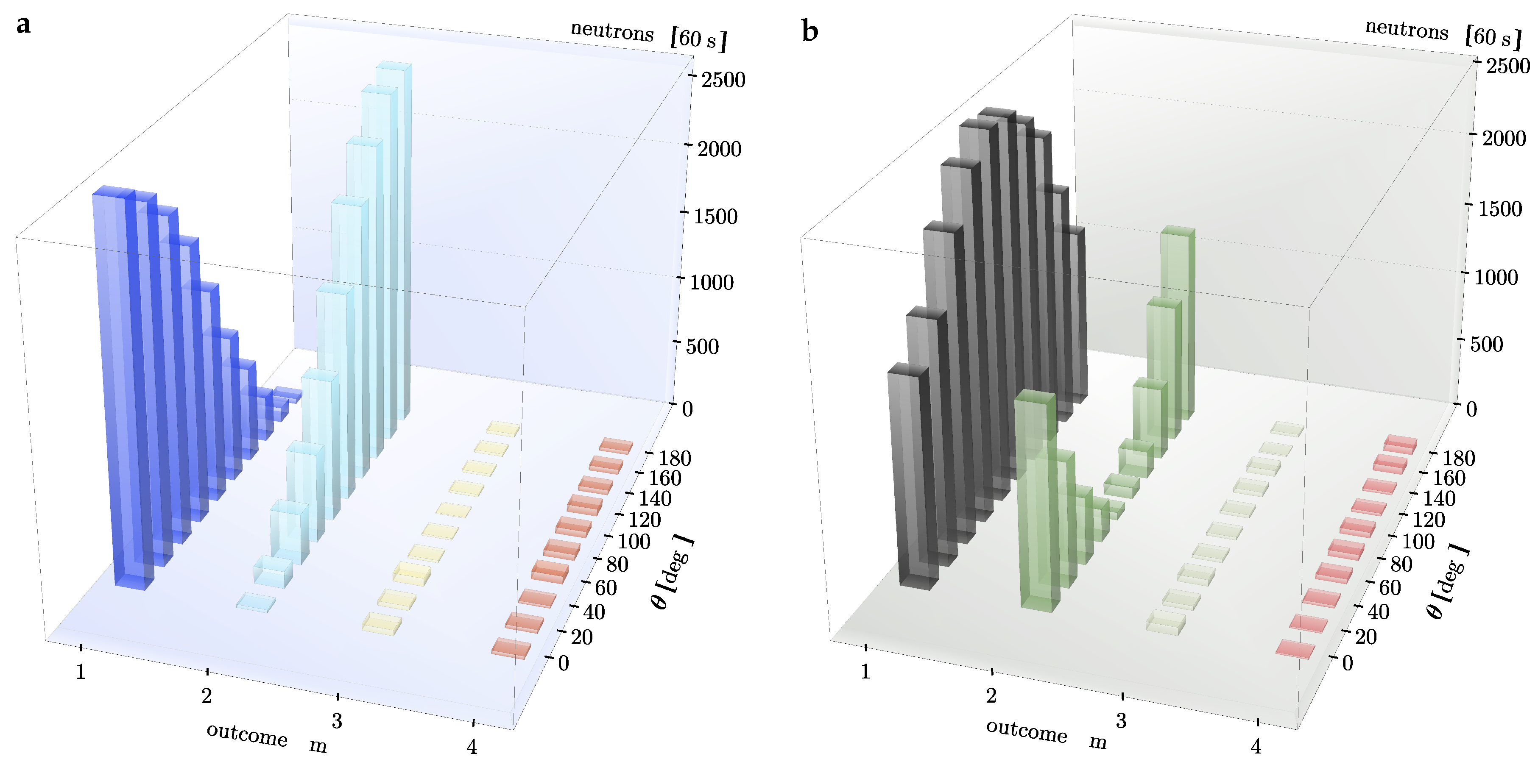
3. Measurement of Entropic Noise–Noise Uncertainty Relation
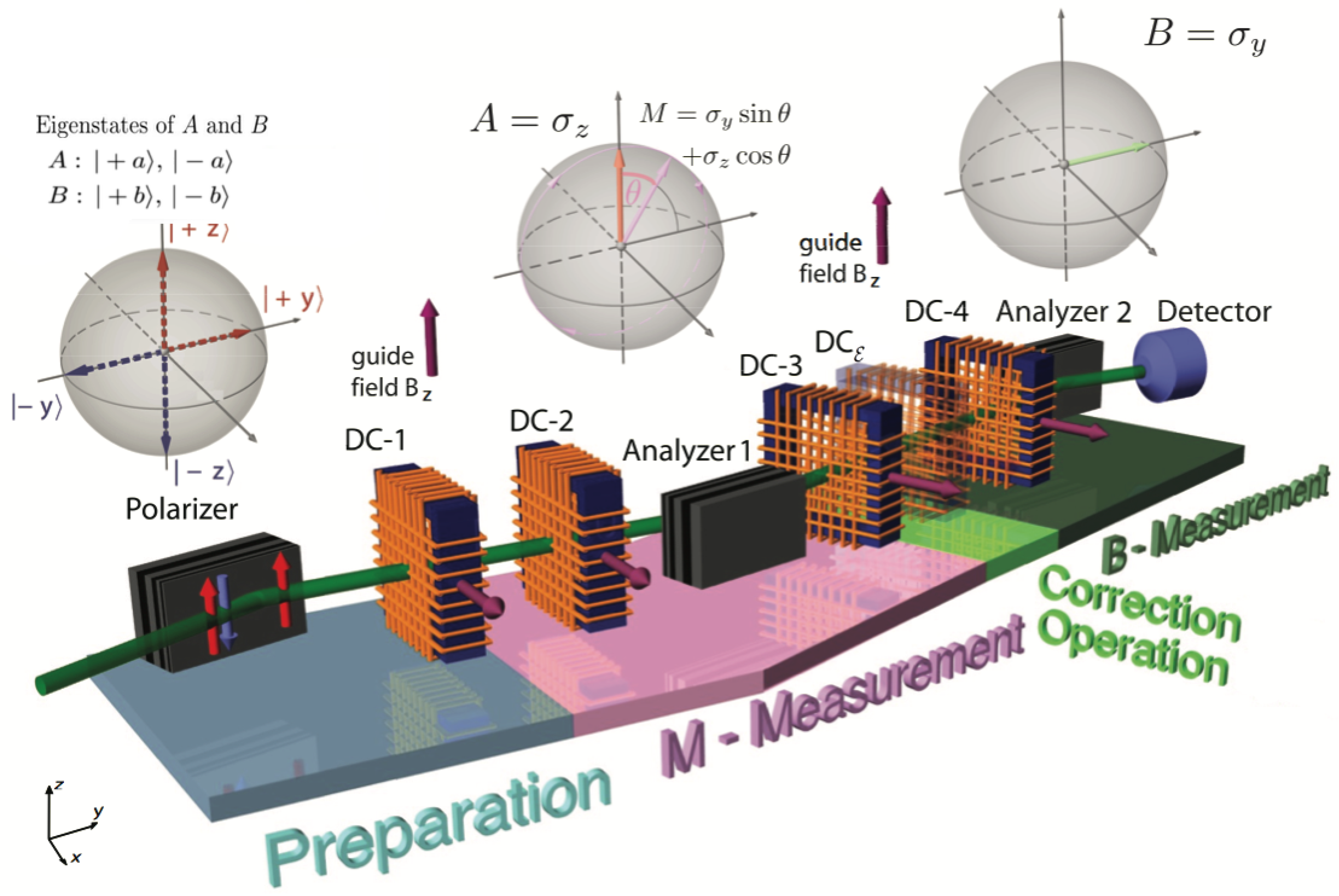
3.1. Set-Up
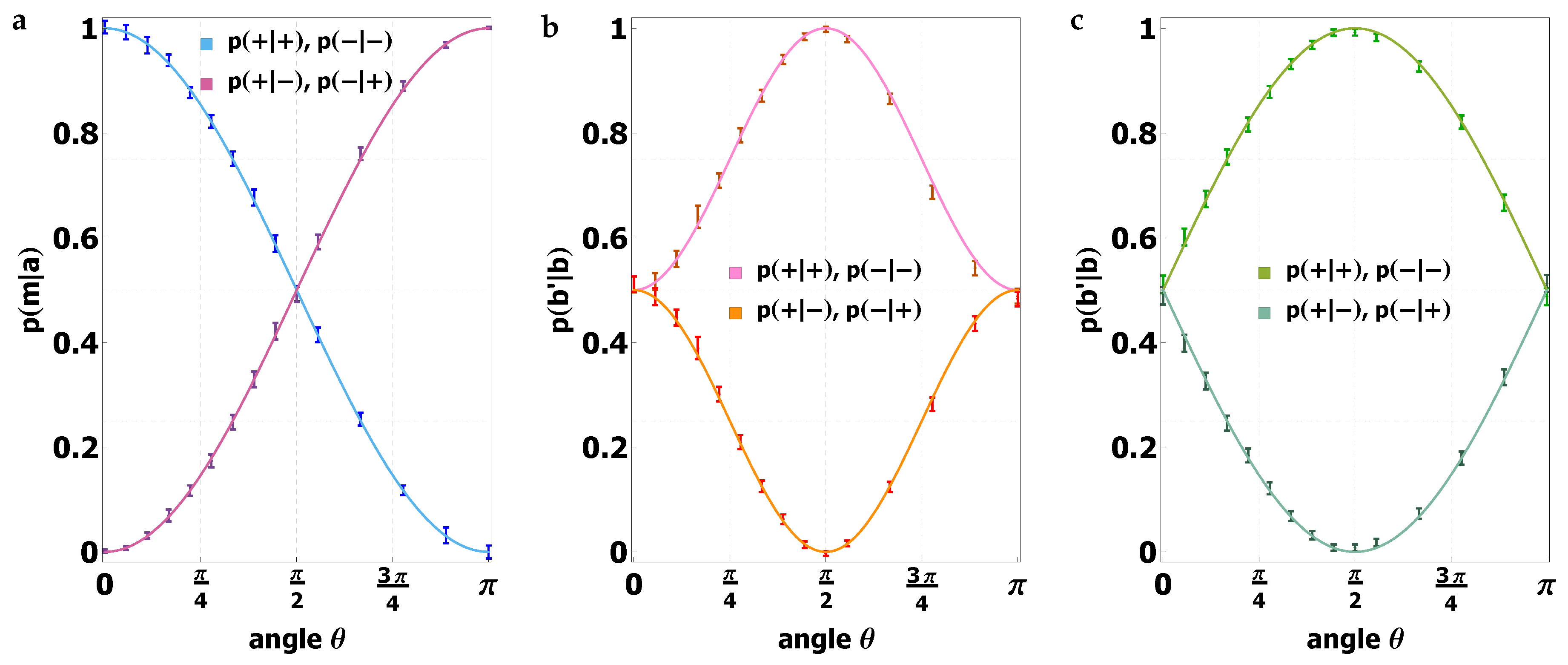
3.2. Measurement Results
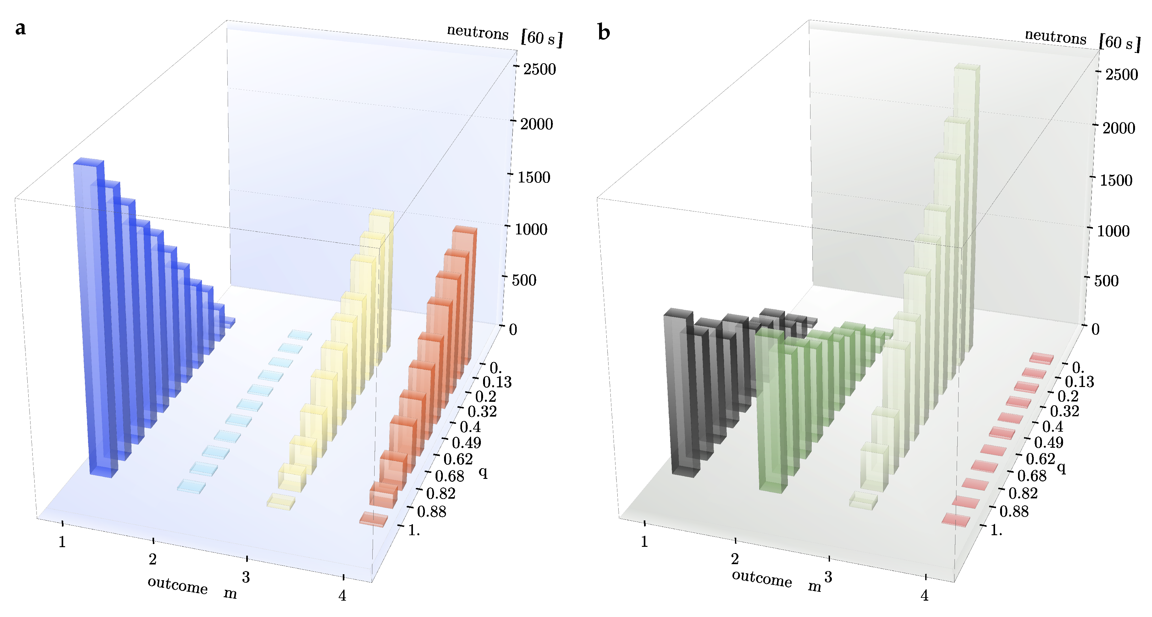
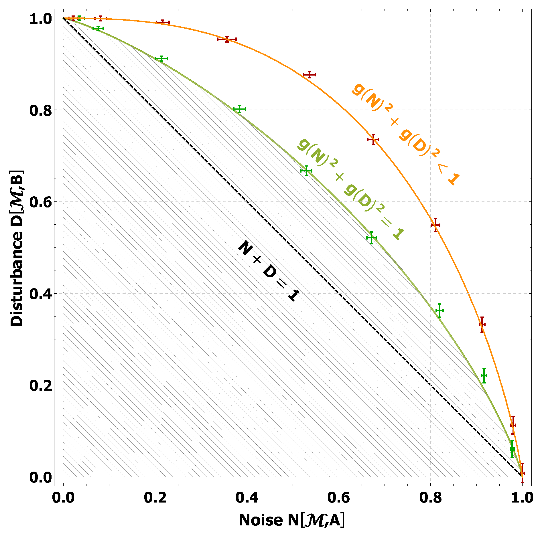
4. Measurement of Entropic Noise–Disturbance Uncertainty Relation
4.1. Set-Up
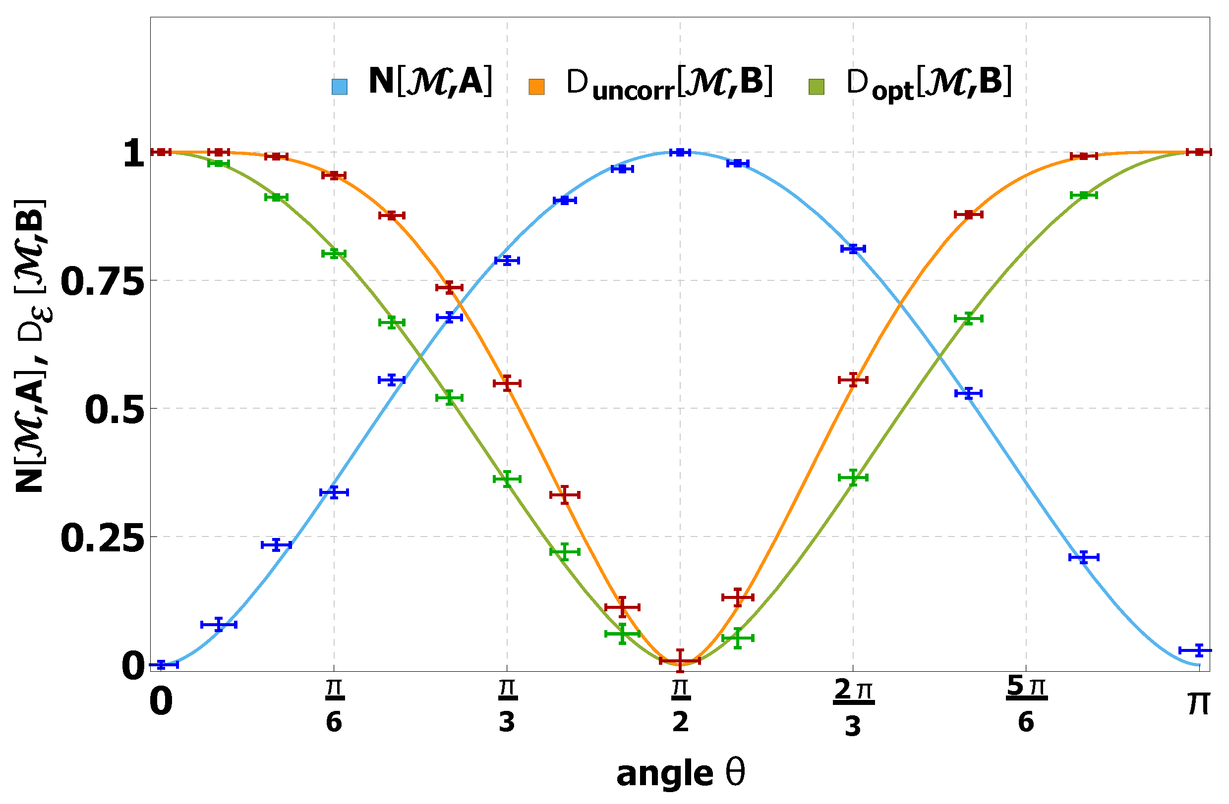
4.2. Measurement Results
5. Conclusions
Author Contributions
Funding
Acknowledgments
Conflicts of Interest
References
- Heisenberg, W. Über den anschaulichen Inhalt der quantentheoretischen Kinematik und Mechanik. Z. Phys. 1927, 43, 172–198. [Google Scholar] [CrossRef]
- Kennard, E.H. Zur Quantenmechanik einfacher Bewegungstypen. Z. Phys. 1927, 44, 326–352. [Google Scholar] [CrossRef]
- Honarasa, G.; Tavassoly, M.; Hatami, M. Number-phase entropic uncertainty relations and Wigner functions for solvable quantum systems with discrete spectra. Physics Letters A 2009, 373, 3931–3936. [Google Scholar] [CrossRef]
- Mandilara, A.; Cerf, N.J. Quantum uncertainty relation saturated by the eigenstates of the harmonic oscillator. Phys. Rev. A 2012, 86, 030102. [Google Scholar] [CrossRef]
- Dammeier, L.; Schwonnek, R.; Werner, R.F. Uncertainty relations for angular momentum. New J. Phys. 2015, 17, 093046. [Google Scholar] [CrossRef]
- Robertson, H.P. The Uncertainty Principle. Phys. Rev. 1929, 34, 163–164. [Google Scholar] [CrossRef]
- Schrödinger, E. Zum Heisenbergschen Unschärfeprinzip. Sitzungsberichte der Preussischen Akademie der Wissenschaften, Physikalisch-mathematische Klasse 1930, 14, 296–303. Available online: http://arxiv.org/abs/quant-ph/9903100 (accessed on 25 December 2019).
- Coles, P.J.; Berta, M.; Tomamichel, M.; Wehner, S. Entropic uncertainty relations and their applications. Rev. Mod. Phys. 2017, 89, 015002. [Google Scholar] [CrossRef]
- Uffink, J.B.M.; Hilgevoord, J. Uncertainty principle and uncertainty relations. Found. Phys. 1985, 15, 925–944. [Google Scholar] [CrossRef]
- Hilgevoord, J. The standard deviation is not an adequate measure of quantum uncertainty. Am. J. Phys. 2002, 70, 983. [Google Scholar] [CrossRef]
- Hirschman, I.I. A Note on Entropy. Am. J. Math. 1957, 79, 152. [Google Scholar] [CrossRef]
- Beckner, W. Inequalities in Fourier Analysis. Ann. Math. 1975, 102, 159–182. [Google Scholar] [CrossRef]
- Biaynicki-Birula, I.; Mycielski, J. Uncertainty relations for information entropy in wave mechanics. Commun. Math. Phys. 1975, 44, 129. [Google Scholar] [CrossRef]
- Deutsch, D. Uncertainty in Quantum Measurements. Phys. Rev. Lett. 1983, 50, 631–633. [Google Scholar] [CrossRef]
- Maassen, H.; Uffink, J.B.M. Generalized entropic uncertainty relations. Phys. Rev. Lett. 1988, 60, 1103–1106. [Google Scholar] [CrossRef]
- Ozawa, M. Universally valid reformulation of the Heisenberg uncertainty principle on noise and disturbance in measurement. Phys. Rev. A 2003, 67, 042105. [Google Scholar] [CrossRef]
- Ozawa, M. Uncertainty relations for noise and disturbance in generalized quantum measurements. Ann. Phys. 2004, 311, 350–416. [Google Scholar] [CrossRef]
- Busch, P.; Lahti, P.; Werner, R.F. Proof of Heisenberg’s Error-Disturbance Relation. Phys. Rev. Lett. 2013, 111, 160405. [Google Scholar] [CrossRef]
- Busch, P.; Lahti, P.; Werner, R.F. Colloquium: Quantum root-mean-square error and measurement uncertainty relations. Rev. Mod. Phys. 2014, 86, 1261–1281. [Google Scholar] [CrossRef]
- Dressel, J.; Nori, F. Certainty in Heisenberg’s uncertainty principle: Revisiting definitions for estimation errors and disturbance. Phys. Rev. A 2014, 89, 022106. [Google Scholar] [CrossRef]
- Erhart, J.; Sponar, S.; Sulyok, G.; Badurek, G.; Ozawa, M.; Hasegawa, Y. Experimental demonstration of a universally valid error-disturbance uncertainty relation in spin-measurements. Nat. Phys. 2012, 8, 185–189. [Google Scholar] [CrossRef]
- Rozema, L.A.; Darabi, A.; Mahler, D.H.; Hayat, A.; Soudagar, Y.; Steinberg, A.M. Violation of Heisenberg’s Measurement-Disturbance Relationship by Weak Measurements. Phys. Rev. Lett. 2012, 109, 100404. [Google Scholar] [CrossRef]
- Sulyok, G.; Sponar, S.; Erhart, J.; Badurek, G.; Ozawa, M.; Hasegawa, Y. Violation of Heisenberg’s error-disturbance uncertainty relation in neutron-spin measurements. Phys. Rev. A 2013, 88, 022110. [Google Scholar] [CrossRef]
- Baek, S.Y.; Kaneda, F.; Ozawa, M.; Edamatsu, K. Experimental violation and reformulation of the Heisenberg’s error-disturbance uncertainty relation. Sci. Rep. 2013, 3, 2221. [Google Scholar] [CrossRef]
- Kaneda, F.; Baek, S.Y.; Ozawa, M.; Edamatsu, K. Experimental Test of Error-Disturbance Uncertainty Relations by Weak Measurement. Phys. Rev. Lett. 2014, 112, 020402. [Google Scholar] [CrossRef]
- Ringbauer, M.; Biggerstaff, D.N.; Broome, M.A.; Fedrizzi, A.; Branciard, C.; White, A.G. Experimental Joint Quantum Measurements with Minimum Uncertainty. Phys. Rev. Lett. 2014, 112, 020401. [Google Scholar] [CrossRef]
- Ma, W.; Ma, Z.; Wang, H.; Chen, Z.; Liu, Y.; Kong, F.; Li, Z.; Peng, X.; Shi, M.; Shi, F.; et al. Experimental Test of Heisenberg’s Measurement Uncertainty Relation Based on Statistical Distances. Phys. Rev. Lett. 2016, 116, 160405. [Google Scholar] [CrossRef]
- Demirel, B.; Sponar, S.; Sulyok, G.; Ozawa, M.; Hasegawa, Y. Experimental Test of Residual Error-Disturbance Uncertainty Relations for Mixed Spin-1/2 States. Phys. Rev. Lett. 2016, 117, 140402. [Google Scholar] [CrossRef]
- Sulyok, G.; Sponar, S. Heisenberg’s error-disturbance uncertainty relation: Experimental study of competing approaches. Phys. Rev. A 2017, 96, 022137. [Google Scholar] [CrossRef]
- Buscemi, F.; Hall, M.J.W.; Ozawa, M.; Wilde, M.M. Noise and Disturbance in Quantum Measurements: An Information-Theoretic Approach. Phys. Rev. Lett. 2014, 112, 050401. [Google Scholar] [CrossRef]
- Sulyok, G.; Sponar, S.; Demirel, B.; Buscemi, F.; Hall, M.J.W.; Ozawa, M.; Hasegawa, Y. Experimental Test of Entropic Noise-Disturbance Uncertainty Relations for Spin-1/2 Measurements. Phys. Rev. Lett. 2015, 115, 030401. [Google Scholar] [CrossRef]
- Abbott, A.A.; Branciard, C. Noise and disturbance of qubit measurements: An information-theoretic characterization. Phys. Rev. A 2016, 94, 062110. [Google Scholar] [CrossRef]
- Demirel, B.; Sponar, S.; Abbott, A.A.; Branciard, C.; Hasegawa, Y. Experimental test of an entropic measurement uncertainty relation for arbitrary qubit observables. New J. Phys. 2019, 21, 013038. Available online: https://arxiv.org/abs/1711.05023 (accessed on 25 December 2019). [CrossRef]
- Shannon, C.E. A mathematical theory of communication. Bell Syst. Tech. J. 1948, 27, 379–423. [Google Scholar] [CrossRef]
- Davies, E.B.; Lewis, J.T. An operational approach to quantum probability. Comm. Math. Phys. 1970, 17, 239–260. [Google Scholar] [CrossRef]
- Sánches-Ruiz, J. Optimal entropic uncertainty relation in two-dimensional Hilbert space. Phys. Lett. A 1998, 244, 189–195. [Google Scholar] [CrossRef]
- Ghirardi, G.; Marinatto, L.; Romano, R. An optimal entropic uncertainty relation in a two-dimensional Hilbert space. Phys. Lett. A 2003, 317, 32–36. [Google Scholar] [CrossRef]
- Bialynicki-Birula, I. Rényi Entropy and the Uncertainty Relations. AIP Conf. Proc. 2007, 889, 52–61. [Google Scholar] [CrossRef]
- Coles, P.J.; Colbeck, R.; Yu, L.; Zwolak, M. Uncertainty Relations from Simple Entropic Properties. Phys. Rev. Lett. 2012, 108, 210405. [Google Scholar] [CrossRef]
- Wilk, G.; Włodarczyk, Z. Uncertainty relations in terms of the Tsallis entropy. Phys. Rev. A 2009, 79, 062108. [Google Scholar] [CrossRef]
- Rastegin, A.E. Uncertainty and certainty relations for complementary qubit observables in terms of Tsallis’ entropies. Quantum Inf. Process. 2013, 12, 2947–2963. [Google Scholar] [CrossRef]
- Barchielli, A.; Gregoratti, M.; Toigo, A. Measurement Uncertainty Relations for Position and Momentum: Relative Entropy Formulation. Entropy 2017, 19, 301. [Google Scholar] [CrossRef]
- Coles, P.J.; Kaniewski, J.; Wehner, S. Equivalence of wave-particle duality to entropic uncertainty. Nat. Commun. 2014, 5, 5814. [Google Scholar] [CrossRef]
- Horodecki, R.; Horodecki, P.; Horodecki, M. Quantum α-entropy inequalities: independent condition for local realism? Phys. Lett. A 1996, 210, 377–381. [Google Scholar] [CrossRef]
- Cerf, N.J.; Adami, C. Entropic Bell inequalities. Phys. Rev. A 1997, 55, 3371–3374. [Google Scholar] [CrossRef]
- Ollivier, H.; Zurek, W.H. Quantum Discord: A Measure of the Quantumness of Correlations. Phys. Rev. Lett. 2001, 88, 017901. [Google Scholar] [CrossRef] [PubMed]
- Winter, A.; Yang, D. Operational Resource Theory of Coherence. Phys. Rev. Lett. 2016, 116, 120404. [Google Scholar] [CrossRef]


© 2020 by the authors. Licensee MDPI, Basel, Switzerland. This article is an open access article distributed under the terms and conditions of the Creative Commons Attribution (CC BY) license (http://creativecommons.org/licenses/by/4.0/).
Share and Cite
Demirel, B.; Sponar, S.; Hasegawa, Y. Measurements of Entropic Uncertainty Relations in Neutron Optics. Appl. Sci. 2020, 10, 1087. https://doi.org/10.3390/app10031087
Demirel B, Sponar S, Hasegawa Y. Measurements of Entropic Uncertainty Relations in Neutron Optics. Applied Sciences. 2020; 10(3):1087. https://doi.org/10.3390/app10031087
Chicago/Turabian StyleDemirel, Bülent, Stephan Sponar, and Yuji Hasegawa. 2020. "Measurements of Entropic Uncertainty Relations in Neutron Optics" Applied Sciences 10, no. 3: 1087. https://doi.org/10.3390/app10031087
APA StyleDemirel, B., Sponar, S., & Hasegawa, Y. (2020). Measurements of Entropic Uncertainty Relations in Neutron Optics. Applied Sciences, 10(3), 1087. https://doi.org/10.3390/app10031087