Defect Detection in Striped Images Using a One-Dimensional Median Filter

Featured Application

The algorithm developed in the research can be applied in any industry that requires a defect detection technique applied to images with a striped background.

Abstract

Defect detection is a key element of quality assurance in many modern manufacturing processes. Defect detection methods, however, often involve a great deal of time and manual work. Image processing has become widely used as a means of reducing the required detection time and effort in manufacturing. To this end, this study proposes an image-processing algorithm for detecting defects in images with striped backgrounds—defect types include scratches and stains. In order to detect defects, the proposed method first pre-processes images and rotates them to align the stripes horizontally. Then, the images are divided into two parts: blocks and intervals. For the blocks, a one-dimensional median filter is used to generate defect-free images, and the difference between the original images and the defect-free images is calculated to find defects. For the intervals, defects are identified using image binarization. Finally, the method superposes the results found in the blocks and intervals to obtain final images with all defects marked. This study evaluated the performance of the proposed algorithm using 65 synthesized images and 20 actual images. The method achieved an accuracy of 97.2% based on the correctness of the defect locations. The defects that could not be identified were those whose greyscales were very close to those of the background.

1. Introduction

Defect detection is one of the important applications of optical inspection. Due to the increasing demand for factory automation, defect detection can be found in many industry sectors. Although the images from different sectors have different characteristics, the way to find defects for the images from one sector may be useful for those from the others. Ngan et al. [1] reported the image processing methods that can be used to find defects on fabric, which usually has repeated patterned texture. They categorized the methods into the statistical approaches, the spectral approaches, the model-based approaches, the learning approaches, and the structural approaches. These approaches are also used in the semiconductor industry. Wang et al. [2] used the statistical approach by proposing the partial information correlation coefficient (PICC) to improve the traditional normalized cross correlation coefficient (TNCCC) for defect detection. They subtracted the standard image from the inspection image to obtain the grayscale difference, calculated the PICC, and compared the PICC with a threshold. If the PICC is less than the threshold, then it indicates that a defect exists. Li et al. [3] used the level-set method to segment the functional regions from light-emitting diode (LED) wafer images after multiple iterations and then used the median value of the average intensities to differentiate different regions for inspection. Ma et al. [4] proposed a generic defect detection method, which analyzes the gray-level-fluctuating conditions of an image and changes the local thresholds according to the conditions. Then the thresholds can be used to segment the defects from the background by using the image difference.

Regarding the spectral approaches, Liu et al. [5] used the spectral subtraction method based on the one-dimensional fast Fourier transform (1-D FFT) to recover the standard defect-free image from three images with defects. The defects could then be detected by comparing the images with defects to the standard image. The advantage of this method is its robustness to illumination. Bai et al. [6] used the phase-only Fourier transform (POFT) to find the salient regions in an image, and then used the template comparison method at the regions to find defects. Unlike traditional template comparison methods, this method is not so sensitive to misalignment between the two images compared. Yeh et al. [7] used the two-dimensional wavelet transform for defect detection by calculating the interscale ratio from the wavelet transform modulus sum (WTMS). Because the ratio of the defect is very different from that of a defect-free image, the defect can be found using an appropriate threshold for the interscale ratio. This approach is template free, so it is easy to implement.

Regarding the deep learning solutions for defect detection, Chang et al. [8] proposed a neural network solution for defect detection on LED wafers. First, the contextual-Hopfield neural network was used to find each die on the wafer, and then they used the mask to segment the light-emitting area and p-electrode from the die. The features of these two areas were extracted. Finally, the Radial Basis Function Neural Network (RBFNN) was used to find the defects. Kyeong and Kim [9] used convolutional neural networks (CNNs) to classify mixed-type defects in wafer bin maps (WBMs). They compared two training methods: one trained each defect type in a separate model, and then combined the results from all models. The other trained only one model with all the possible mix-type defects. They found that using the former yielded better accuracy. Their experimental results showed that the CNN outperformed the support vector machine (SVM) and the multilayer perceptron (MLP). The accuracy achieved using CNN was about 91%, compared to the accuracy of 72% using SVM, and 45% using MLP.

In addition to its application in the semiconductor-related industry, defect detection using image processing can also be found in other industries. To segment an infection location on green leaves, Singh and Misra [10] first used the G-plane in RGB images to remove the image background. They then used a genetic algorithm to find the connected regions and used a color co-occurrence matrix to find the texture features for disease classification. Yang [11] proposed an image analysis technique with the help of a set of evenly spaced parallel light stripes to find apple stems and calyxes. The stems and calyxes can be identified because the continuous parallel light stripes near them became unparalleled, broken, or deformed. Lai et al. [12] adopted a similar idea by using structured light to enhance the transparent defects for easy detection on a polymeric polarizer. Lee et al. [13] proposed to use the 2D Discrete Fourier transform and a local threshold binarization method for TFT-LCD defect inspection. The method can effectively find defects in the pad areas with patterns of varying frequencies. Liu et al. [14] enhanced strip steel images using an enhancement operator based on mathematical morphology (EOBMM), which can reduce the effects of uneven illumination. Then, a genetic algorithm was applied to the binarization of the defect images. The method outperformed the commonly used Otsu method and Bernsen method based on the three error matrices presented in their research.

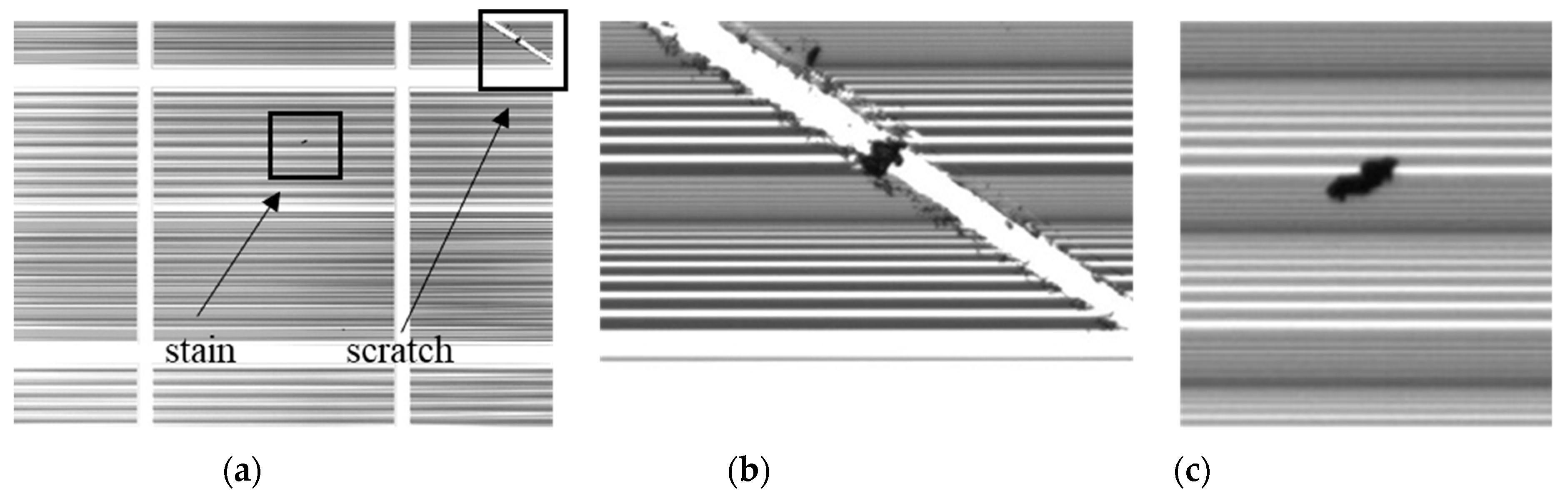
Based on the discussion above, and to the best of the authors’ knowledge, little consideration has been given to detect imaging defects in the background of striped blocks. In this study, defects in images from a semiconductor manufacturing company had to be detected. The defects, including scratches and stains, exist in the images with the background of striped blocks. Therefore, the purpose of this study was to develop an image-processing algorithm for effectively detecting defects in such images. The proposed algorithm may also be used in some other applications, such as defect detection using the structured light of stripe patterns.

2. Materials and Methods

2.1. Equipment and Images

The algorithm developed in this research was implemented with Python 3.6 and OpenCV 3 running on a Windows 7 operating system on a PC with an Intel Xeon 3.2-GHz CPU and 18 GB of RAM. The images to be inspected were 8-bit 4096 × 3072 pixel grayscale images. One of the images is illustrated in Figure 1a. The striped background feature is obvious. The defects can be categorized into two types: scratches, as shown in Figure 1b, and stains, as shown in Figure 1c. Scratches and stains may exist in the same image, as shown in Figure 1a. The minimum number of pixels for stains was about 80, but the number of pixels for the scratches varied. From Figure 1a, there are also stripe-free areas, which look like the number sign #. These are referred to as intervals in this paper. The striped areas between the intervals are referred to as blocks. There are nine connected blocks in each of the images processed. While there may appear to be 12 blocks in Figure 1a, the top portions of the middle three blocks are connected to their bottom portions, respectively, so that there are only nine connected blocks. The heights and the widths of the intervals between the blocks were constant in all images, but the sizes of the blocks varied. This study took advantage of the fixed-sized intervals of the images in the proposed algorithm.

2.2. One-Dimensional Median Filter

The two-dimensional median filter is commonly used in image processing to remove salt-and-pepper noises. Due to the characteristics of striped images in this research, this study extended the two-dimensional median filter to a one-dimensional median filter to remove the noises along with the stripes. The idea is similar to that of the temporal median filter used in [15]. The application of the one-dimensional median filter is explained as follows. In order to obtain the one-dimensional array, as shown in Figure 2, it is first necessary to find the median of the grayscale values of all elements. Then, the grayscale values of all the elements are replaced with the median. It is then possible to calculate the difference between the new array and the original array, and the elements with significant discrepancies could be noises.

2.3. Flow of Defect Detection

The flow of defect detection is shown in Figure 3. To use the one-dimensional median filter effectively, the grayscale values of the elements in each row must be as consistent as possible. Therefore, pre-processing and image rotation are required to align the stripes in the image horizontally. Image segmentation is then performed to obtain the block images and the interval images. Defect detection can then be conducted on the blocks and the intervals separately, and finally the results can be superposed to complete the task. The process is described in detail below.

2.3.1. Pre-Processing and Image Rotation

The pre-processing flow is shown in Figure 4. First, a Gaussian filter is used to smooth the image, and histogram equalization is used to reduce the uneven brightness. Then, Gamma correction is used to enhance the contrast. Finally, binarization and image complement are performed to make the blocks foreground. Using the vertices of the middle block of the processed image, we can determine the rotation angle, and the stripes in the image can be rotated to the horizontal to facilitate the subsequent median filtering.

2.3.2. Image Segmentation

The image segmentation process is shown in Figure 5. The purpose of this step is to segment the image into blocks and intervals, because different approaches are used for defect detection in blocks and intervals in the paper. The image shown in Figure 6a is used to explain the step. First, all connected blocks are identified, as shown by the red boundaries in Figure 7a, and the bounding box that can contain an entire connected block must be calculated for each block. All the connected blocks were marked from one to nine, as shown in Figure 7. The bounding boxes, shown as green boxes in Figure 7b, can be used as masks to separate the blocks and intervals. The masks for the blocks based on the bounding boxes, shown in Figure 7b, are illustrated in Figure 7c. Due to the influence of the defect circled in Figure 7b, the bounding box in the middle is incorrect. To remove the effect of the defect on the bounding boxes, we can take the following approach: For the three connected blocks, blocks 2, 5, 8, the x-coordinate value of the leftmost pixel in each row of these blocks can be obtained, and the median of all the values obtained can be used as the x-coordinate of the bounding box on the left-hand side of connected blocks 2, 5, and 8. By using the same way, we can find all the other sides of the bounding boxes for all the connected blocks. Because the number of pixels of all the defects in an entire image is less than 1% of the total pixels for all the images we have, this approach can correctly find all the bounding boxes.

As explained previously, the spacing between the blocks in each image is the same. After measuring the pixel distance of the image spacing, we found that x_d1 = x_d2 = 85 pixels and y_d1 = y_d2 = 135 pixels, as shown in Figure 6b. From the correct bounding boxes and the fixed block spacing, the blocks and intervals can be correctly segmented.

Figure 8a shows the mask for the blocks. When the mask is applied to the image shown in Figure 6a, the image of the blocks can be segmented, as shown in Figure 8b. The red circle indicates a defect in the block.

The mask for the intervals, shown in Figure 9a, can be obtained by complementing Figure 8a. When Figure 9a is applied to the original image, as shown in Figure 6a, the image of the intervals can be segmented, as shown in Figure 9b. The red circle indicates a defect in the interval.

2.3.3. Defect Detection in Blocks

After the image is segmented, defect detection for blocks can be conducted. The flow is shown in Figure 10. The median filtering is applied to the block images first to generate the standard defect-free images. The median filtering cannot remove large stains, so the large stains must be processed using a different approach. Then the proposed method subtracts the defect-free image from the original image to find the defects in the blocks. The details of the step are described below.

As shown in Figure 11, each block image is divided into several sections with a width of m pixels. How to determine the value of m is discussed in the next section. Applying the one-dimensional median filtering row by row in each section of a block image, a defect-free block image is obtained if there are no large stains. Here, Section 1 in Figure 11 is used as an example. Figure 12a shows the image before and after the one-dimensional median filtering is applied. It can be seen that the defects are removed.

For large stains, if the number of pixels with stains in a row is greater than half of the section width m, then the grayscale values of the whole row will be replaced by the grayscale value of the stain, and the one-dimensional median filtering fails. The situation is illustrated in Figure 12b. Therefore, another approach is required for large stains. According to statistics of the images provided, the lowest grayscale value for the background pixels was about 80, and the grayscale value for the large stains was about 40. Therefore, if the grayscale difference was greater than 40, it meant that there was a large stain. After the locations of the large stains are found, the appropriate threshold for image binarization can be used on the original images to obtain the locations of the large stains.

Other defects, such as small stains and scratches, are detected by applying image subtraction to the original defect images and the defective-free images. The defect-free images, which are processed by the one-dimensional median filter, should have grayscale values similar to those of the original images, with the exception at defect locations. Therefore, after image subtraction, image binarization can be used to locate the defects. Here, Block 5, shown in Figure 13, is used as an example. Figure 13a shows the original defect image, and Figure 13b shows the image after the one-dimensional median filter has been applied to remove the defects. Subtracting Figure 13b from Figure 13a and using image binarization on the result yields the image shown in Figure 14a, in which the white defects (red circled) are identified. Conversely, subtracting Figure 13a from Figure 13b and using image binarization on the result yields the image shown in Figure 14b, in which the black defects (red circled) are identified. How to determine the binarization threshold, T_r, will be discussed in the next section. All defects in blocks can thus be found using the procedure described above for all blocks.

2.3.4. Defect Detection in Intervals

The flow of defect detection in intervals is shown in Figure 15. The interval segmentation result is first obtained, as shown in Figure 16a, and then the mask for the blocks, as shown in Figure 16b, obtained in Section 2.3.2, is added to the segmented interval image, thus identifying the defects in the intervals as shown in Figure 17a.

Because the image does not necessarily rotate to the position where each stripe in the image is perfectly horizontal, line noises may exist, as shown in Figure 17a. The closing operation is thus used on the image to remove some of the noises, and image binarization and image complement are performed to generate a noise-free image, as shown in Figure 17b, which is the result of defect detection in the intervals. Here, T_w denotes the binarization threshold, and how to determine its value is discussed in the next section.

After defect detection on blocks and intervals is complete, the resulting images are superposed to obtain the defect detection results for the entire image.

3. Results and Discussion

Due to the limited number of actual defect images, the algorithm was evaluated based on 20 actual images and 65 synthesized images. The synthesized images were constructed using the segmented defects from the actual images, and the defects were randomly rotated and placed at various locations in defect-free images to synthesize the defect images. At most, two defects were included in each of the synthesized images.

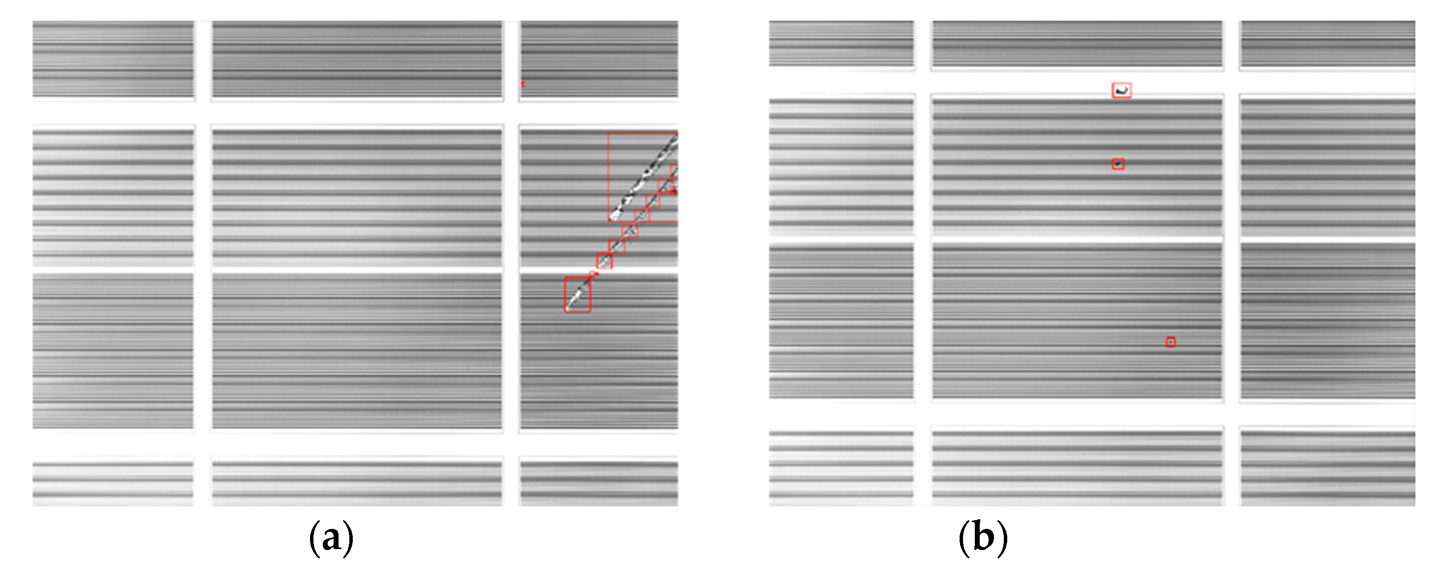
Figure 18 illustrates two examples of the results obtained using the proposed algorithm. The scratches and stains were all identified and marked in Figure 18a,b, respectively. The processing time for an image was approximately 6.9 s.

Tasi and Rivera Molina [16] used the false negative rate (FNR) and the false positive rate (FPR) to determine two thresholds. FNR and FPR are defined in Equation (1) and Equation (2) as follows:

$$FNR=\frac{FN}{TP+FN},$$

(1)

$$FPR=\frac{FP}{FP+TN},$$

(2)

where False Negative (FN) is the number of instances in which there is a defect but the proposed algorithm fails to identify it; True Positive (TP) is the number of instances in which there is a defect and the proposed algorithm correctly finds it; False Positive (FP) is the number of instances in which there are no defects but the proposed algorithm incorrectly determines that there is one; and True Negative (TN) is the number of instances in which there are no defects and the proposed algorithm correctly determines that there are none.

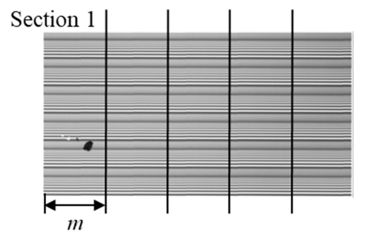
By fixing one threshold, Tasi and Rivera Molina [16] tested in which case the other threshold could reach the lowest FNR and FPR. This study used a similar process to determine two critical parameters: section width, m, and block binarization threshold, T_r.

A total of 30 actual images, which were not from the 85 test images, were used to determine the two parameters, m and T_r so that FNR and FPR were as small as possible. Here, this study adopted the root sum square (RSS) of FNR and FPR as the objective to be minimized.

First, this study set T_r to be 15 and found the RSS of FNR and FPR for m ranging from 200 to 450, in increments of 50. The results are shown in

Table 1. Root sum square of false negative rate (FNR) and false positive rate (FPR) when m varied from 200 to 450 and T_r = 15.

m	200	250	300	350	400	450
RSS of FNR and FPR	0.283	0.283	0.281	0.284	0.283	0.285

. It can be seen that when m = 300, the RSS had its minimum value of 0.281. Besides, the RSS varied little when m was in the range. In other words, FNR and FPR are not sensitive to m. Next, this study used m = 300 and found the RSS of FNR and FPR for T_r, ranging from 5 to 35, in increments of 5. As shown in

Table 2. Root sum square of FNR and FPR when T_r varied from 5 to 35 and m = 300.

Tr	5	10	15	20	25	30	35
RSS of FNR and FPR	1.002	0.439	0.321	0.303	0.336	0.388	0.424

, when T_r = 20, the RSS was at its minimum, so T_r = 20 was used in the proposed algorithm.

Finally, the binarization threshold (T_w) was determined. When T_w ranged from 185 to 215 with an increment of 5, the RSS was at its minimum when T_w = 190, as shown in

Table 3. Root sum square of FNR and FPR when T_w varied from 185 to 215.

Tw	185	190	195	200	205	210	215
RSS of FNR and FPR	0.135	0.109	0.112	0.122	0.129	0.167	0.429

, so T_w was set to 190 in this research.

After the three critical parameters were determined, the performance of the algorithm was evaluated with 20 actual images and 65 synthesized images based on TPR, FPR, and Accuracy (ACC). TPR is defined as:

$$TPR=\frac{TP}{TP+FN}$$

(3)

and ACC is defined as:

$$ACC=\frac{TP+TN}{TP+FP+FN+TN}.$$

(4)

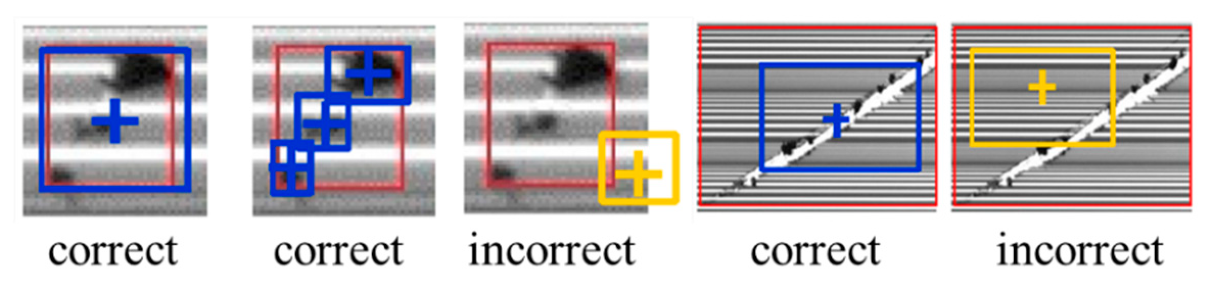
The evaluation criteria were based on the bounding box and its center, as shown in Figure 19. The red bounding box is the correct position, and the blue or yellow bounding boxes are the results obtained by the proposed algorithm. If the position of the center was off the correct position, it was considered a failed defect detection. If the found bounding box was not completely consistent with the red bounding box, but the center of both boxes matched well, it was considered correct. There were 126 defects in the 85 images. Positive was defined as a defective region; negative was defined as a defect-free region. For defect detection, the number of defect regions could be counted, but not the number of defect-free regions. To make the subsequent calculation possible, this study assumed that there were as many defect-free regions as defect regions, which was equal to 126. The results achieved using the algorithm are listed in

Table 4. Evaluation results of 126 defects in 85 images.

No. of Defective Regions	TP	FN	FP	TN	TPR	FPR	ACC
126	119	7	0	126	94.4%	0%	97.2%

. The TP value was 119, which meant that the proposed algorithm correctly detected 119 of 126 defects. The remaining seven defects that could not be detected were the FN cases. The FP value was 0, which meant that the proposed algorithm had sufficient robustness for noises that it did not generate any false positives. Using Equations (2) and (3), the FPR was 0%, and the TPR was 94.4%. Using Equation (4) yielded an accuracy of 97.2% [17].

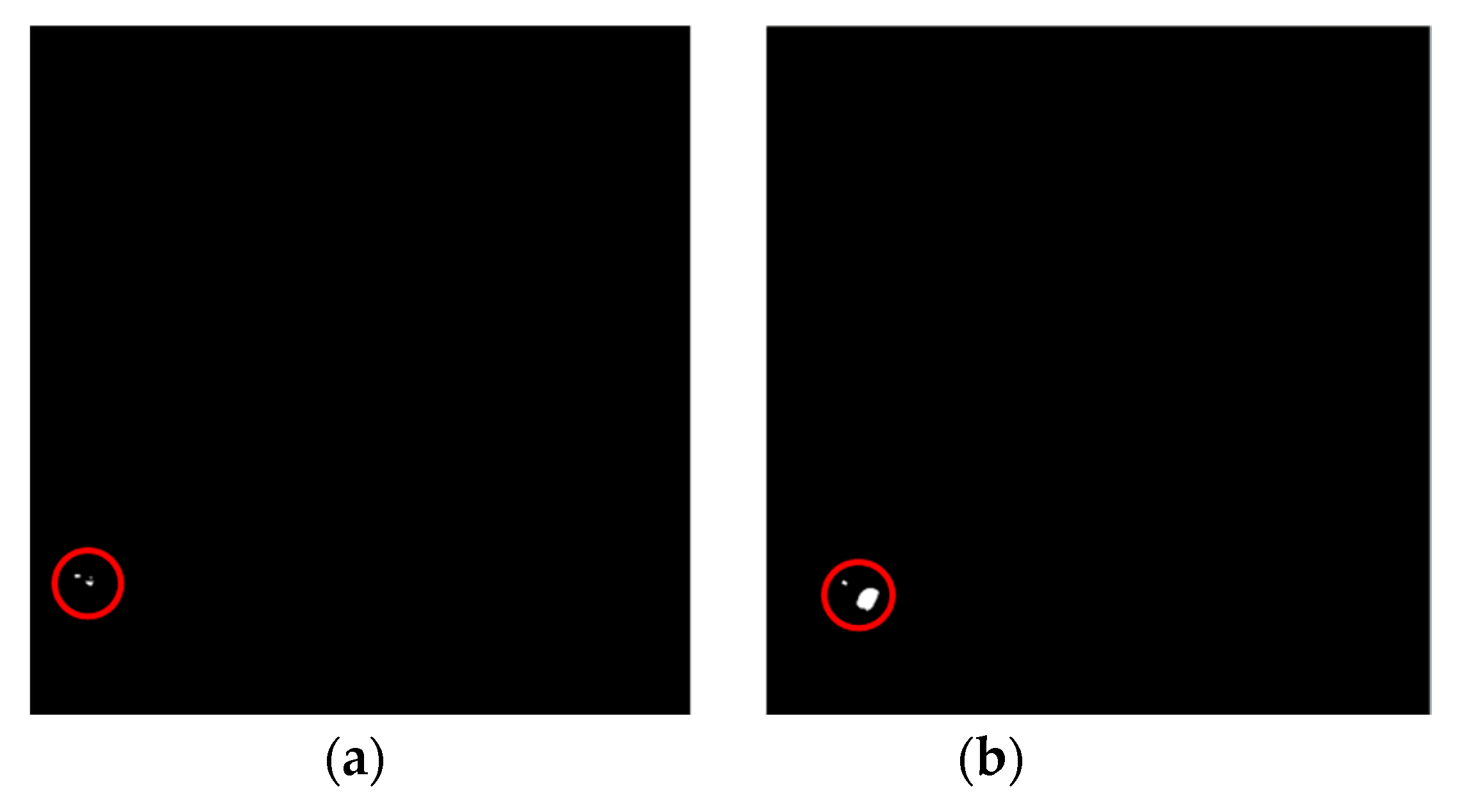
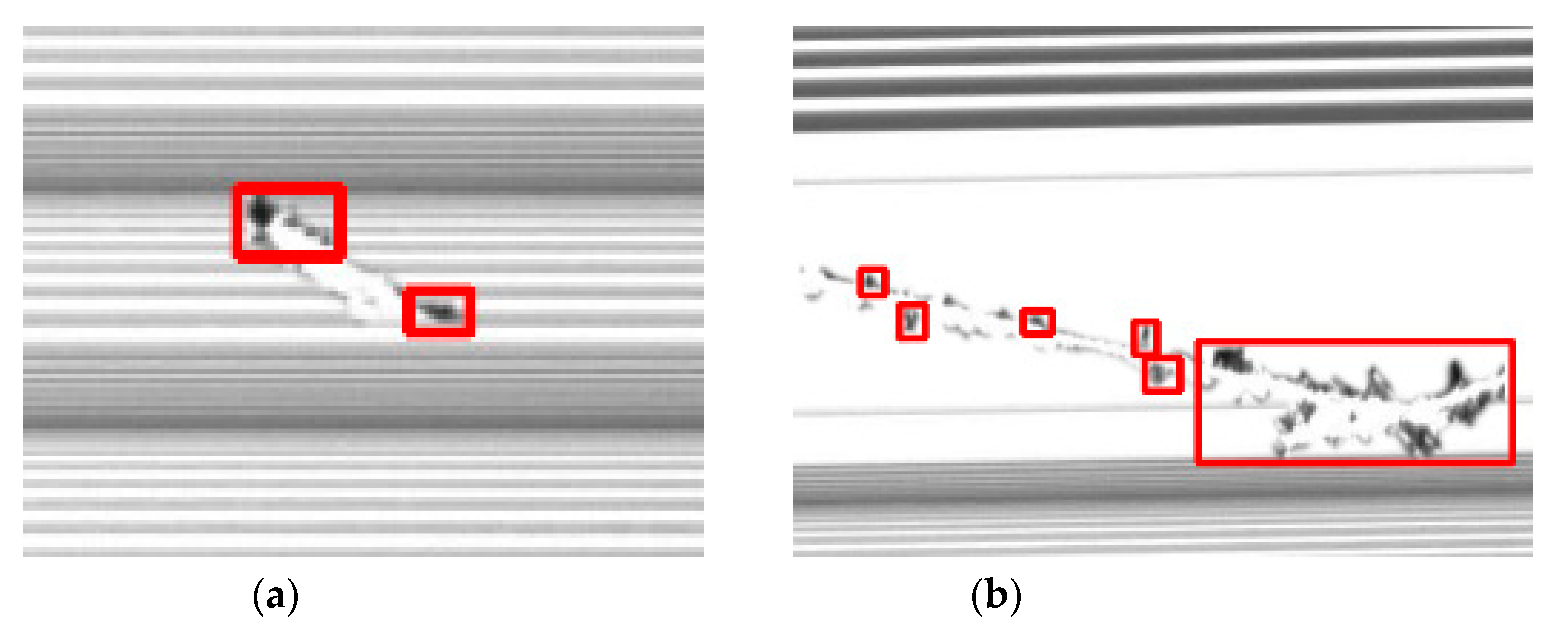
This study analyzed the seven defects that were not detected by the proposed algorithm. The seven defects occurred in six images. These defects were all scratches. From the enlarged views shown in Figure 20, it can be seen that only the black portions of the scratches were detected, while their white portions were not. This failure was because the grayscale values of the white portions were close to the grayscale values of the background. Therefore, the proposed algorithm may fail to detect scratches whose grayscale values are too close to those of the background.

4. Comparison to Other Study

Here we used the deep learning method to detect defects and compare the results with those obtained by using the proposed method in the paper. The deep learning model was Faster R-CNN with ResNet-101, and the pre-trained model was on the MS COCO dataset. The number of images used for training and validation, the learning rates, and the total training steps are listed in

Table 5. Summary of deep learning setup.

No. of synthesized images used	Training dataset: 30,159 Validation dataset: 7500
Learning rates	Initial, 0.0003 Steps > 50,000, 0.00003 Steps > 100,000, 0.000003
Total training steps	184,914

. Due to the limited number of the images we have, we synthesized the images for training and validation with 128 different defects on 18 different defect-free images. We arbitrarily chose a defect and put it at a location on one of the 18 defect-free images to obtain a synthesized image. By using different combinations of the defect, the defect-free image, and defect location, we synthesized about 40,000 images in total. Among them, 30,159 images were used for training and 7500 images for validation. The validation accuracy was greater than 99%.

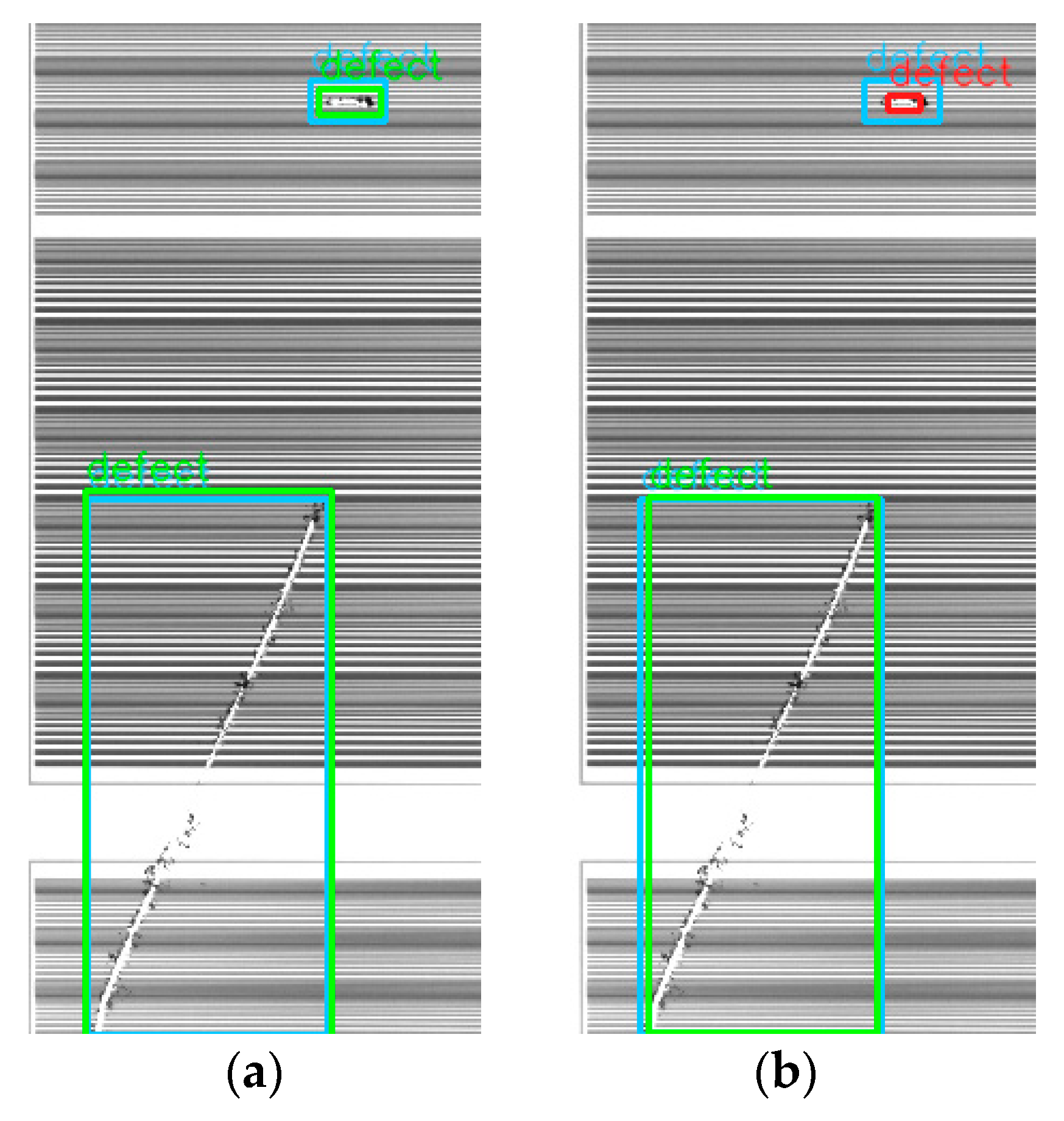
After obtaining the trained model, we applied both methods to 83 images with defects and used 0.5 as the intersection over union (IOU) threshold. The average precision (AP) for the proposed method was 0.91, and that for the deep learning method was 0.74. One image with the defect detection results is shown in Figure 21. From the figure, we can see that the defect detection by using the proposed method can correctly find the bounding boxes of the two defects in the image, but the deep learning method failed to find one. For other images, the deep learning method even missed some defects. The training dataset may cause the deep learning results with lower AP. Although we used about 30,000 images for training, the amount and the variety may not be enough to yield high AP. From the observation of the deep learning results, most of the poor predictions are related to missing defects and imprecise bounding boxes. The method proposed in this paper finds defects using the image difference, which is more robust to find the defects.

5. Conclusions

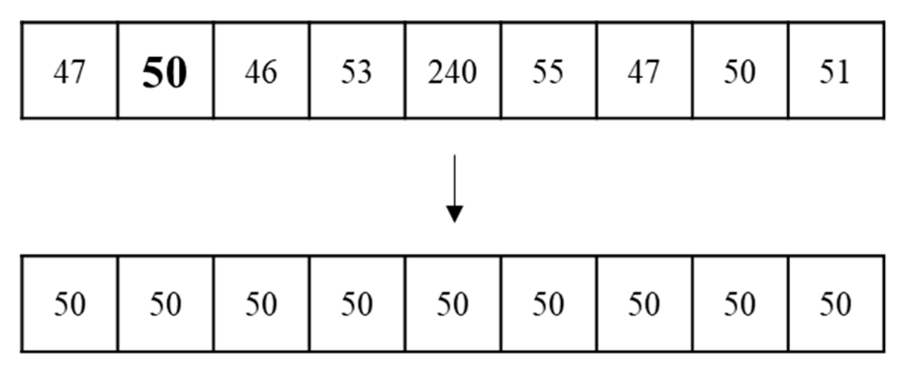
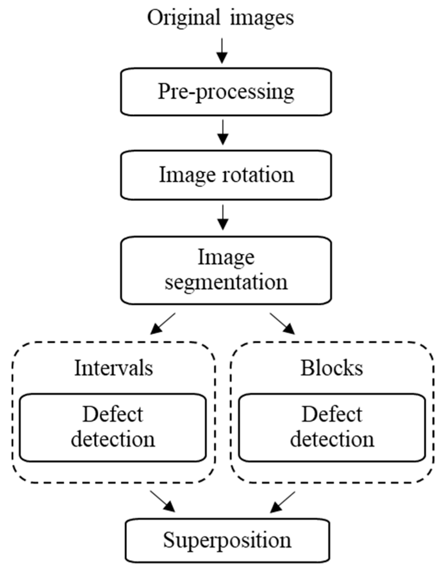
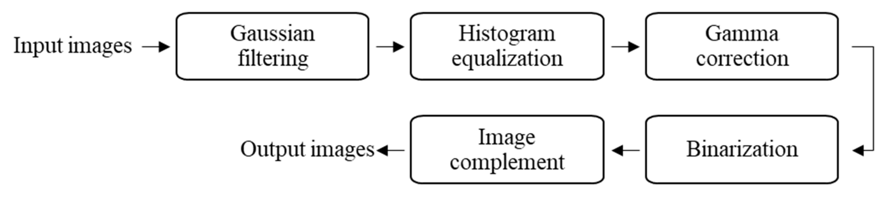
This study proposed a defect detection method for striped images using a one-dimensional median filter. After pre-processing and horizontal alignment image rotation, images were segmented into blocks and intervals. Defects were then found for the blocks and the intervals, respectively. To identify block defects, we used a one-dimensional median filter to generate standard defect-free images. The difference between the standard image and the original image was then used to find the defects. To identify interval defects, we used the image binarization to highlight the defects. Finally, the defect detection results for the blocks and intervals were superposed to obtain all the defects in the entire image. The experiment results show that the proposed method achieved an accuracy of 97.2% based on the correctness of the defect regions. The results demonstrate that the algorithm proposed in this study can effectively detect defects and correctly mark their positions. The proposed method was compared with the deep learning method, and the results show that the average precision by using the proposed method was 0.91 and that by using the deep learning method was 0.74. The proposed method has better robustness in terms of finding the correct bounding boxes for the defects.

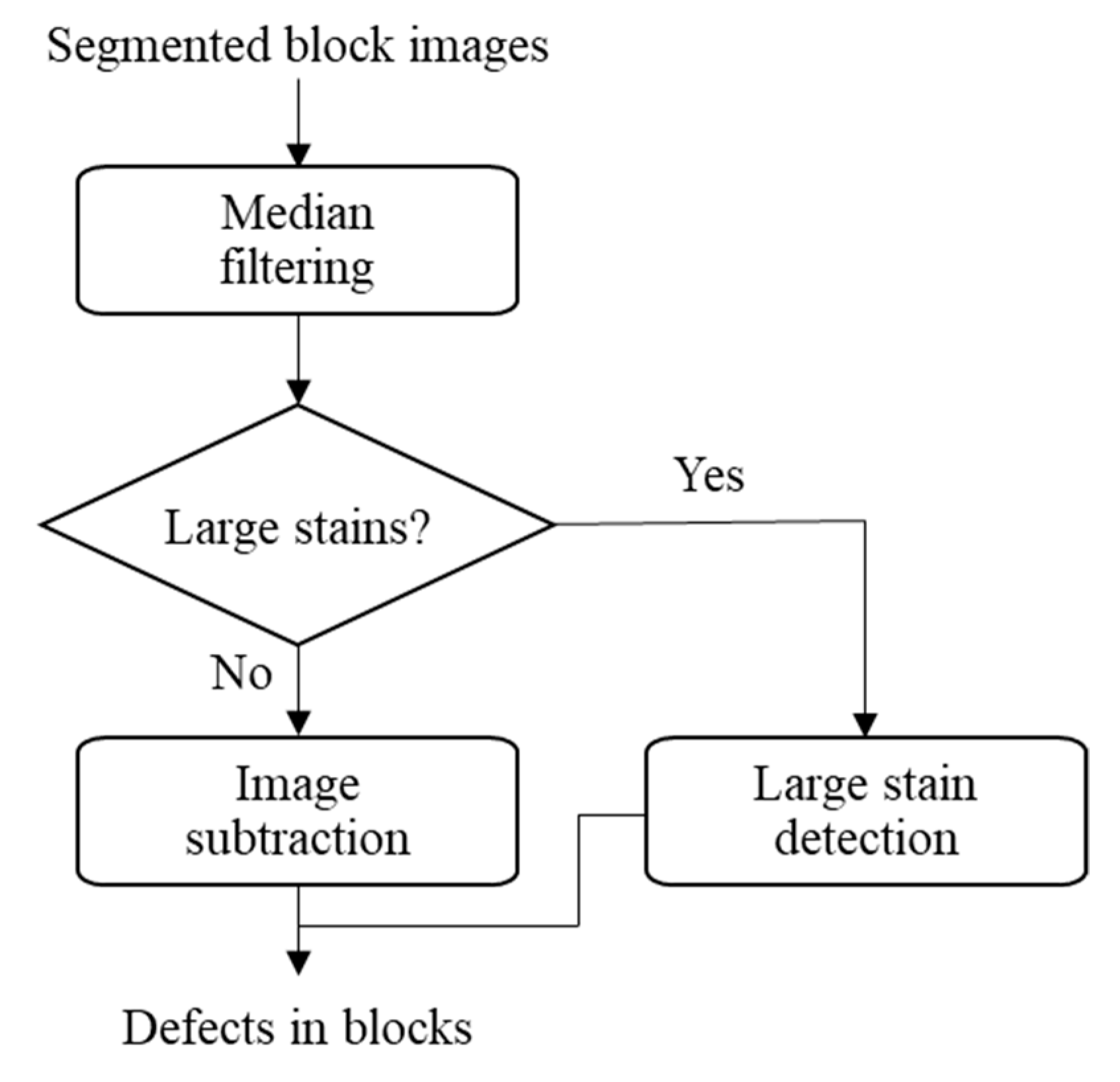
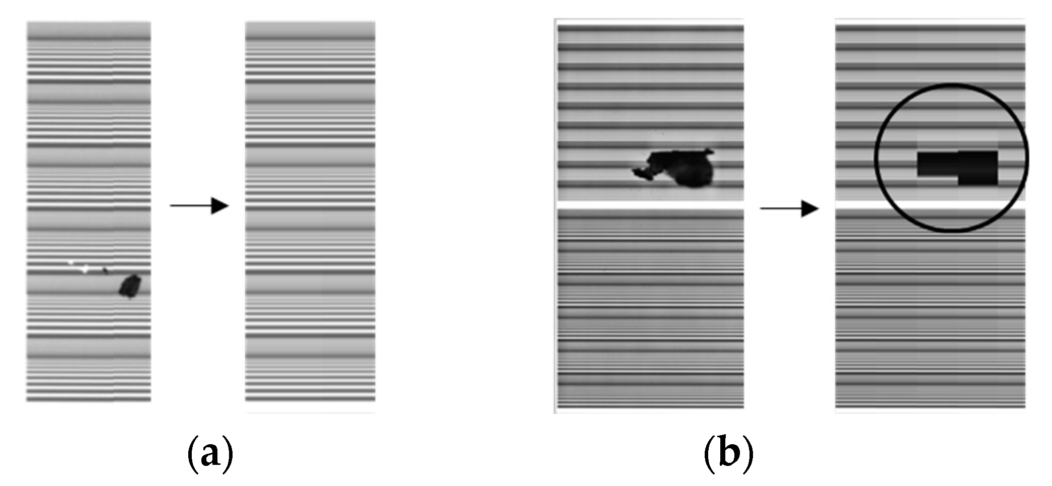
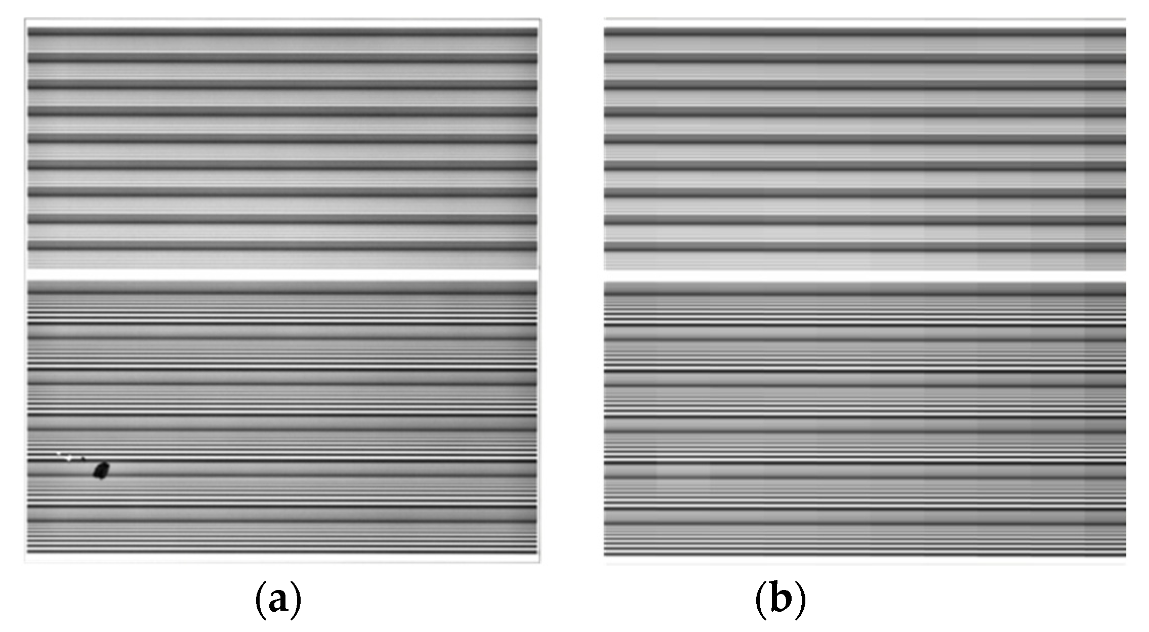
The algorithm used in this paper was developed based on the stripe characteristics of the images. If the images do not have stripes, the algorithm cannot be used. In addition, the stains need to be small (less than m/2 as discussed in the paper), which is valid for the given images. For large stains, it may not be possible to apply the median filter to recover the defect-free images. However, as long as there are some columns in a block that are not affected by the large stains, we can still use the periodic characteristics caused by the stripes along the y-direction in the stain-free columns to recover the defect-free images, which can be used to detect the large stains. However, a lot of noises will also be found. Then a particle analysis can help identify the large stains. This algorithm can be developed as a supplement to the algorithm proposed in the paper so that we can use the proposed algorithm in the paper to find the small defects and then use the supplement to find the large defects. The extension of the proposed algorithm to cover large defects and the optimization of the algorithm to reduce the processing time will be the topics for our future work.

References

1. Ngan, H.Y.T.; Pang, G.K.H.; Yung, N.H.C. Automated fabric defect detection—A review. Image Vis. Comput. 2011, 29, 442–458. [Google Scholar] [CrossRef]
2. Wang, C.C.; Jiang, B.C.; Lin, J.Y.; Chu, C.C. Machine vision-based defect detection in IC images using the partial information correlation coefficient. IEEE Trans. Semicond. Manuf. 2013, 26, 378–384. [Google Scholar] [CrossRef]
3. Li, C.H.; Chang, C.Y.; Jeng, M. Applying regional level-set formulation to postsawing four-element LED wafer inspection. IEEE Trans. Syst. Man Cybern. Part C 2011, 41, 842–853. [Google Scholar] [CrossRef]
4. Ma, Y.; Li, Q.; Zhou, Y.; He, F.; Xi, S. A surface defects inspection method based on multidirectional gray-level fluctuation. Int. J. Adv. Robot. Syst. 2017, 14, 1729881417703114. [Google Scholar] [CrossRef] [Green Version]
5. Liu, H.; Zhou, W.; Kuang, Q.; Cao, L.; Gao, B. Defect detection of IC wafer based on spectral subtraction. IEEE Trans. Semicond. Manuf. 2010, 23, 141–147. [Google Scholar]
6. Bai, X.; Fang, Y.; Lin, W.; Wang, L.; Ju, B.F. Saliency-based defect detection in industrial images by using phase spectrum. IEEE Trans. Ind. Inform. 2014, 10, 2135–2145. [Google Scholar] [CrossRef]
7. Yeh, C.H.; Wu, F.C.; Ji, W.L.; Huang, C.Y. A wavelet-based approach in detecting visual defects on semiconductor wafer dies. IEEE Trans. Semicond. Manuf. 2010, 23, 284–292. [Google Scholar] [CrossRef]
8. Chang, C.Y.; Li, C.H.; Chang, Y.C.; Jeng, M. Wafer defect inspection by neural analysis of region features. J. Intell. Manuf. 2009, 22, 953–964. [Google Scholar] [CrossRef]
9. Kyeong, K.; Kim, H. Classification of mixed-type defect patterns in wafer bin maps using convolutional neural networks. IEEE Trans. Semicond. Manuf. 2018, 31, 395–402. [Google Scholar] [CrossRef]
10. Singh, V.; Misra, A.K. Detection of plant leaf diseases using image segmentation and soft computing techniques. Inf. Process. Agric. 2017, 4, 41–49. [Google Scholar] [CrossRef] [Green Version]
11. Yang, Q. Apple Stem and Calyx Identification with Machine Vision. J. Agric. Eng. Res. 1996, 63, 229–236. [Google Scholar] [CrossRef]
12. Lai, W.-W.; Zeng, X.-X.; He, J.; Deng, Y.-L. Aesthetic defect characterization of a polymeric polarizer via structured light illumination. Polym. Test. 2016, 53, 51–57. [Google Scholar] [CrossRef] [Green Version]
13. Lee, J.-Y.; Kim, T.-W.; Pahk, H.J. Robust defect detection method for a non-periodic TFT-LCD pad area. Int. J. Precis. Eng. Manuf. 2017, 18, 1093–1102. [Google Scholar] [CrossRef]
14. Liu, M.; Liu, Y.; Hu, H.; Nie, L. Genetic algorithm and mathematical morphology based binarization method for strip steel defect image with non-uniform illumination. J. Vis. Commun. Image Represent. 2016, 37, 70–77. [Google Scholar] [CrossRef]
15. Liu, W.; Cai, Y.; Zhang, M.; Li, H.; Gu, H. Scene background estimation based on temporal median filter with Gaussian filtering. In Proceedings of the 23rd International Conference on Pattern Recognition, Cancun, Mexico, 4–8 December 2016; pp. 132–136. [Google Scholar]
16. Tsai, D.M.; Rivera Molina, D.E. Morphology-based defect detection in machined surfaces with circular tool-mark patterns. Measurement 2019, 134, 209–217. [Google Scholar] [CrossRef]
17. Tai, P.-L. Defect Detection on Striped Images by Using a One-Dimensional Median Filter. Master Thesis, National Taiwan University of Science and Technology, Taipei, Taiwan, August 2019. [Google Scholar]
Figure 1. Defects in the striped images include: (a) scratches and stains (marked with boxes). (b) Enlargement of a scratch. (c) Enlargement of a stain.
Applsci 10 01012 g001
Figure 2. (Top) The original one-dimensional array, in which the median of all the elements is 50. (bottom) The new one-dimensional array consists of the median, 50, for all its elements.
Applsci 10 01012 g002
Figure 3. Flow of the overall defect detection algorithm for striped images.
Applsci 10 01012 g003
Figure 4. Flow of pre-processing.
Applsci 10 01012 g004
Figure 5. Flow of image segmentation.
Applsci 10 01012 g005
Figure 6. (a) The original image with defects in the middle block and the intervals; (b) the block numbers and the widths of the intervals are illustrated.
Applsci 10 01012 g006
Figure 7. (a) The red lines and curves are the boundaries of the connected blocks, and a defect is marked with a blue circle; (b) the green boxes are the bounding boxes of the connected blocks; (c) The mask obtained by the bounding boxes in (b) is affected by the defect circled in (a,b).
Applsci 10 01012 g007
Figure 8. (a) The mask for the blocks. (b) The image of the blocks segmented using the mask in (a) and a defect is marked with a red circle.
Applsci 10 01012 g008
Figure 9. (a) The mask for the intervals. (b) The image of the intervals segmented using the mask in (a) and the defect is marked with a red circle.
Applsci 10 01012 g009
Figure 10. Flow of defect detection in blocks.
Applsci 10 01012 g010
Figure 11. Block image divided into sections with width m pixels.
Applsci 10 01012 g011
Figure 12. Applying the one-dimensional median filtering to the block image can remove small defects in (a) but cannot remove the large defects in (b).
Applsci 10 01012 g012
Figure 13. (a) Original image of Block 5; (b) the defect-free image of (a) obtained by using one-dimensional median filtering.
Applsci 10 01012 g013
Figure 14. (a) Results of subtracting Figure 13b from Figure 13a; (b) results of subtracting Figure 13a from Figure 13b.
Applsci 10 01012 g014
Figure 15. Flow of defect detection in intervals.
Applsci 10 01012 g015
Figure 16. (a) Segmented interval image; (b) Mask for the blocks.
Applsci 10 01012 g016
Figure 17. (a) Image with defects and noises; (b) Applying closing operation, binarization, and image complement to (a) to remove the noises and identify defects in the interval.
Applsci 10 01012 g017
Figure 18. (a) Scratches and (b) stains were identified and marked by the proposed algorithm.
Applsci 10 01012 g018
Figure 19. Evaluation criteria for regional comparison.
Applsci 10 01012 g019
Figure 20. The enlarged scratches that the proposed algorithm failed to detected: (a) in the block, and (b) in the interval.
Applsci 10 01012 g020
Figure 21. The detected defects in an image by using (a) the proposed method and (b) the deep learning method. The blue bounding box represents the ground truth; the gree one represents the bounding box predicted correctly, and the red one represents the bounding box predicted incorrectly.
Applsci 10 01012 g021