Discontinuity Capture in One-Dimensional Space Using the Numerical Manifold Method with High-Order Legendre Polynomials

Abstract

Traditional methods such as the finite difference method, the finite element method, and the finite volume method are all based on continuous interpolation. In general, if discontinuity occurred, the calculation result would show low accuracy and poor stability. In this paper, the numerical manifold method is used to capture numerical discontinuities, in a one-dimensional space. It is verified that the high-degree Legendre polynomials can be selected as the local approximation without leading to linear dependency, a notorious “nail” issue in Numerical Manifold Method. A series of numerical tests are carried out to evaluate the performance of the proposed method, suggesting that the accuracy by the numerical manifold method is higher than that by the later finite difference method and finite volume method using the same number of unknowns.

1. Introduction

Discontinuity is a very common phenomenon in fluid flow. For example, high speed fluids can produce shock waves when they pass from subsonic to supersonic speeds. Another example is the separation of two fluids of different materials by a thin film, which can also produce a discontinuity when the film is pulled out. Discontinuities are also commonly found in convection-dominated flows, and this type of discontinuity plays a very important role in fluid dynamics. Therefore, extensive research was carried out [1,2,3,4,5]. At present, in computational fluid dynamics, dealing with shock wave problems is mainly achieved by directly solving Navier-Stokes equations by increasing the computing power of the computer, such as quantum computing [6], or solving molecular dynamics problems [7,8]. However, such calculation conditions are difficult to achieve in engineering. The Methods commonly used in engineering will be discussed in detail later.

There are several numerical methods commonly used at present. The finite element method (FEM) is a numerical method that discretizes the entire problem area into units, constructs interpolation functions on the units, and solves the unknowns by Galerkin method and the principle of variation. The finite element method is a very good method for continuous solids. However, in order to solve the solid with cracks and discontinuities, the finite element method needs to refine the mesh during the solution process, which is not only complicated, but also loses accuracy. In addition, because finite elements cannot satisfy the law of conservation of mass in the element, it is not convenient to be applied in the field of fluids. The finite difference method (FDM) is a numerical method that directly differentiates and discretizes the strong form of the original equation. Because the finite difference method directly discretizes the equation, although it can be applied in the field of fluids, it requires a relatively regular solution area. For complex boundary problems, the finite difference method is not easy to use. The finite volume method (FVM) is a numerical method that uses conservation of momentum and conservation of mass to construct equations based on each volume cell. The finite volume method has the same discrete format and the same accuracy as the finite difference method in the case of a regular grid. However, compared with the finite difference method, the finite volume method can solve the problems in complex regions and complex boundary conditions, while losing a small amount of accuracy. The finite volume method is also one of the most commonly used methods in computational fluid dynamics.

Numerical discontinuity is very common in computational mechanics. The one type of discontinuity is material discontinuity, such as cracks, material interfaces, voids. In addition, another type is numerical discontinuity such as shock waves in hydrodynamics.

The traditional methods mentioned above are all based on continuity hypotheses, in which the displacement and the density are continuous. For the approximation of non-smooth solution, the above methods will result in big errors near singularities, leading to false high gradients. In order to achieve higher accuracy, a very dense deployment of elements or points must be set at the singularities.

However, any effort to study fluid dynamics by numerical simulations must face great challenges in order to get solutions with high accuracy and stability around discontinuities. Finite volume method and finite difference method are commonly used methods of computational fluid dynamics. There are still many problems about FVM and FDM to be resolved: (1) The FVM mesh must be consistent with the discontinuities; (2) The discontinuity is moving during the process of shock wave propagation Special techniques known as artificial dissipation or limiting projection have to be designed in order to avoid the “Gibbs” phenomenon caused by higher order interpolation and its accompanying spurious numerical oscillation.

However, great efforts have to be input to design such techniques. In order to achieve high accuracy near discontinuities, many non-oscillation schemes have been proposed. For example, Monotone Upstream-centered Schemes for Conservation Law (MUSCL), a kind of Total Variation Diminishing (TVD) schemes, avoids numerical oscillations by adding a flow limiter [9]. TVD schemes ensures that the physical field in the transition region is monotonic and bounded, but it does not solve the problem of numerical dissipation.

Numerical manifold methods (NMM) have been invented and applied to numerical computation and engineering by Shi et al. [10]. NMM are capable of dealing with discontinuities in a unified way. In NMM, the mathematical cover can be cut into many physical patches by the solution domain, while the local approximation is constructed directly on the physical patches. The function that constructs the local approximation can be discontinuous, so the numerical manifold method can handle discontinuity problems in a natural way. So far, many problems have been well solved by NMM, such as the seepage problems [11], the wave propagation problems [12], the two-dimensional dynamic crack propagation problems [13,14,15], the three-dimensional crack propagation problems [16], the fourth-order problem [17], the contact problem [18], and so on. It is well known that the analytic solution can be viewed as a higher-order polynomial. The higher the order of expansion, the higher the accuracy of the approximation. The NMM is also based on the partition of unit scheme, the global approximation can be established by multiplying a weight function by local approximations. Like generalized finite elements, numerical manifold methods can construct higher order global approximation by simply raising the order of the local approximations or weight function. Currently, there are two main skills for constructing high accuracy global approximations [19].

At present, the numerical manifold element method is already a very effective method in the solid field, and it is increasingly used in the field of engineering simulation. For example, hydraulic fracturing [20,21], pore medium problem [22,23,24], dynamic consolidation [25], fracture problem [26], slope stability analysis [27].

Although there are a few studies on the numerical manifold element method in fluid mechanics, it has been successfully applied to solve the incompressible and viscous Navier-Stokes equation [28,29]. However, there are no articles about applying numerical manifold element method to fluid discontinuities. Numerical manifold element method has a universal way in solving discontinuous problems, so it is very worthwhile to develop it in the field of fluid mechanics.

Facing fluid mechanics problems with the discontinuity, the interpolation of FDM or FVM will result in the slope at discontinuity. However, the NMM can show great potential to approximate the discontinuity, making it is necessary to develop NMM in fluid mechanics. This paper is an attempt of the numerical manifold element method in the field of computational fluid dynamics with discontinuities.

The main contents of this manuscript are as follows. In Section 2, the foundation of the numerical manifold method is briefly introduced. In Section 3, the construction of local and global approximations is expounded upon. The new scheme for singular patch reconstruction is presented in detail. In Section 4, the discretization of equations is carried out. In Section 5, numerical results of some tests are given and compared with other schemes. The linear dependent issue will be discussed in detail. Some remarks, conclusions, and prospects are presented in Section 6.

2. Foundation of NMM

This section only introduces the basic concepts of NMM, and more details can be found in reference [30]. In order to solve continuous and discontinuous problems in a unified framework, NMM applies two covers, namely the mathematical cover (MC) and the physical cover (PC) [30]. In this manuscript, MC will be constructed by mathematical mesh of a regular segment.

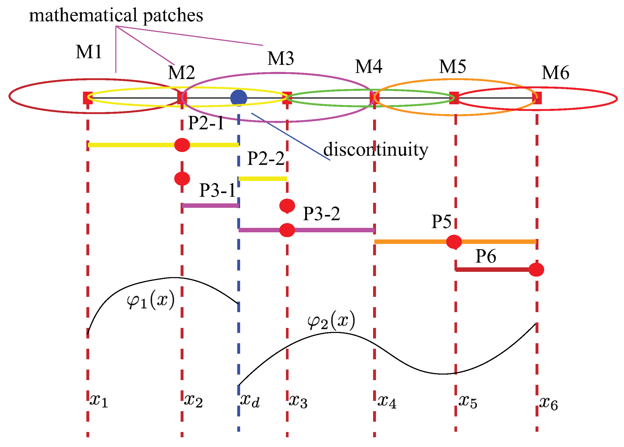
In NMM, MC is composed of a series of simply connected small domains, each of which is named as a mathematical patch (MP), consisting of all the elements or intervals sharing the same node. For example, in Figure 1, the one-dimensional problem domain $\Omega$ is divided into five intervals, each of which has two nodes. M1 (the red circle) and M3 (the purple circle) are MPs. It is noteworthy that in NMM, MC does not have to match the problem domain but needs to cover it, which means that NMM does not have to deploy a mesh that matches the shock waves, making it very suitable for dealing with the discontinuities in problems. For simplicity in presentation, here let nodes M1 and M6 coincide with the problem domain ends

The physical cover is formed by a combination of all the physical patches, which are obtained by cutting all mathematical patches with the problem region components. Here, a problem region component might be boundary segment, a discontinuity or a material interface. Cutting a MP, at least one PP can be generated. In Figure 1, for example, cutting M2 with the discontinuity marked by the blue dot, leads to the generation of $P2-1$ and $P2-2$, marked by yellow segments. Each PP corresponds to a “star point” (also called “NMM node” or “generalized node”) as exhibited with red circles in Figure 1.

In NMM, the local approximation is defined on PPs. That is to say, the degrees of freedom are attached at NMM node. For convenience, the “NMM nodes” in the rest of this article will be referred to as “nodes”. There are two types of $PPs$ in NMM as given in Figure 1. The one type is called non-singular patch which does not contain a crack tip in its domain, such as $PP2$. Another type is singular patch which contains a crack tip in its domain, such as $PP3$ and $PP5$. Different local approximations will be constructed according to different types of physical patches.

In Figure 1 $P1$ is generate by $M1$ cut by left domain boundary, $P2-1$ and $P2-2$ are generated by $M2$ cut by the discontinuity (blue dot). It should be noticed that the physical patches generated by same mathematical patch have different star points at the same position.

3. Construction of Local and Global Approximations

NMM is based on partition of unity (PU), thus the global approximation is obtained by the weighted average of the local approximations of all the physical patches, reading

$${\varphi }^{*}=\sum _{ij}{w}_i{a}_{ij}{L}_{ij}$$

(1)

where $w_i$ is the weight function of the ith mathematical patch, and the subscript i represents the ith mathematical patch. j stands for the jth physical patch cut out of the ith mathematical patch, $L_{ij}$ is the local approximation function, $a_{ij}$ are called generalized degrees of freedom of physical patch j.

The weight function $w_i$ can be any function which just needs to satisfy the PU condition $\sum w_i=1$ and the property of compact support.

The local approximation function can be any function which can express the properties of solution on the physical patch. The polynomial bases are usually chosen, since the polynomial bases are easy and simple to approximate the real solution.

In this study, for convenience, if the weight function is hat function

$$w_i=\frac{1}{2}(\frac{|x-x_c|-|x-x_b|}{|x_c-x_b|}-\frac{|x-x_b|-|x-x_a|}{|x_b-x_a|})$$

(2)

where $x_a$ and $x_c$ are the left and right boundary of ith MP, respectively. $x_b$ is the position of the star point.

The weight function has the $\delta$ property. In Figure 2, the weight function only depends on the mathematical patch, regardless of whether there is discontinuity or not in it.

3.1. Local Approximation of Zero Order

The local approximations are built on the physical patches, so the local approximation can be influenced by discontinuities. In Figure 2, the goal function to be approximated has two parts

$$\phi \left(x\right)=\left\{\begin{array}{cc}\hfill {\phi }_1\left(x\right)& x<x_d\hfill \\ \hfill {\phi }_2\left(x\right)& x\ge x_d\hfill \end{array}\right.$$

(3)

where $x_d$ represents discontinuous position.

The discontinuity at $x_d$ cut the physical patch $P2$ into $P2-1$ and $P2-2$ and cut $P3$ into $P3-1$ and $P3-2$.

We first consider the local approximation on the ordinary physical patches, such as $P5$ in Figure 2, in which no discontinuities exist. There are many options we can choose, such as MLS-based function [31]. Since polynomials can uniformly converge to any continuous function, the polynomials are chosen. The zero-degree Legendre polynomial can be used, namely, $L_{ij}=1$. The global approximation turns out to be linear interpolation

$${\varphi }^{*}=\sum _{ij}{w}_i{a}_{ij}$$

(4)

If the physical patch consists of many parts, such as $P2-1$ and $P2-2$ in Figure 2, the local approximation can be also cut into the same parts. As above, local approximation on $P2$ is first established, and then the parts both $P2-1$ and $P2-2$ inherit the origin function on interval $[x_1,x_d]$ and $[x_d,x_3]$ respectively. The number of star point has increased and the value of star points is different at same position. This property can be used to describe the discontinuity, in which the value of two sides from the interface is different.

3.2. Local Approximation of High Order

The accuracy of the local approximation depends on the size of space. The Legendre polynomials have excellent properties including orthogonality. The orthogonality can adjust the properties of coefficient matrix. The basis function $L_n\left(x\right)$ of n degree will be defined on the interval $[-1,1]$ as

$$L_n\left(x\right)=\frac{1}{2^{n}n!}\frac{{\mathrm{d}}^n}{\mathrm{d}{x}^n}{(x^2-1)}^n$$

(5)

When $n=0$, it is the above case ($L_{ij}=1$). The nodes are uniformly preset in the domain, and star points are located at different positions. The original Legendre polynomials should be moved or scaled to satisfy the boundary of mathematical patch, which can maintain the good properties of Legendre polynomials. Thus, the final high order NMM approximation is

$${\varphi }^{*}=\sum _{ijk}{w}_i{a}_{ij}^k{L}_{ij}^k$$

(6)

where k is the order of Legendre polynomials and $a_{ij}^k$ is the degrees of freedom of the kth order.

The higher order of the polynomials is used, the closer to real solution the approximation will be, due to polynomial base is dense in space $C[a,b]$ (continue function space on interval $[a,b]$).

If discontinuity occurred as mentioned above, the new physical patches generated by old patches and discontinuities will inherit the old function of original patches. In many fields, however, the increased order may result in “linear dependence” (LD) issue, in which the global matrix is rank deficient even after sufficient constraints are coerced. Encouragingly, in this paper, no LD issue is incurred while obtaining high accuracy, which will be verified in follow section.

3.3. Local Approximation on Singular Patch

The purpose of NMM to introduce the mathematical cover lies in generating the weight functions. A better global approximation can be reached by selecting proper local approximations of the physical patches. Therefore, once we know the local behaviors of solution, we can exploit them in the construction the global approximation. Supposing we know the analytical solution near the discontinuity and the the analytical solution in the neighborhood of discontinuity is $g_l\left(x\right)$, we can further use the property of partition of unit and the weight function s, then the global approximation is defined below

$${\varphi }^{*}=\prod _l(1-s_l\left(x\right))\sum _{ijk}{w}_i{a}_{ij}^k{L}_{ij}^k+\sum _l{s}_l\left(x\right)g_l\left(x\right)$$

(7)

where s is the weight function and can be any function that less than or equal to 1. The value of $s_l$ is more than zero at the lth singular patch, but is zero at other domains.

For example, s can be selected as

$$s_l=e^{-k{(x-x_l)}^2}$$

(8)

where k is a positive number, $x_l$ is the position of the lth discontinuity.

4. Discrete Equations

The basic idea of NMM is to construct the local approximation, and further form global approximation. Substituting the global approximation into the original functions or equations can obtain the coefficient $a_{ij}$. Next, we will explain how to construct the solution and the process of solving.

4.1. Known Function with Discontinuities

Suppose the exact solution is $f\left(x\right)$ with discontinuities of first kind and the NMM approximate solution is

$$f^{*}=\sum _{ij}{w}_i{a}_{ij}{L}_{ij}$$

(9)

where the subscript i denotes the ith mathematical patch and j the jth physical patch in each mathematical patch, $L_{ij}$ are Legendre polynomials, and $a_{ij}$ is the value at each star point of physical patch.

To get the weak form of the equation, a test function space must be specified. The form of test function can be any base of compact space on piecewise continuous function space, but not all bases are suitable because LD issue may be caused [32]. Giving the test function space $\left\{w_l{L}_{lm}\right\}$, which will be verified not causing LD problem in the following sections, we will get weak form as below:

$${\int }_{\Omega }{f}^{*}{w}_l{L}_{lm}\mathrm{d}\Omega ={\int }_{\Omega }f{w}_l{L}_{lm}\mathrm{d}\Omega$$

(10)

following that, we can get a linear equations system

$$\left\{\begin{array}{cc}\hfill K_{kn}& =w_i{L}_{ij}{w}_l{L}_{lm}\hfill \\ \hfill b_k& ={\int }_{\Omega }f{w}_l{L}_{lm}\mathrm{d}\Omega \hfill \end{array}\right.$$

(11)

where k and n represent the positions of physical patches, and both of them are closely related to $i,j$ and $l,m$.

Figure 3 gives a method to calculate the coefficient, which is basic in NMM approximating a solution.

This method can easily capture discontinuity, but there are still some problems to be resolved. Like NMM in solid, we must first confirm where discontinuity is. In fracture mechanics, we can determine the position of discontinuity by initial crack and propagation. In hydrodynamics, there are also some methods to determine the position of discontinuity, such as the exact solution of Riemann problem, and the capture of shock wave.

4.2. The Derivative

Some equations contain derivative, such as the advection equation:

$$\frac{\partial u}{\partial t}+\frac{\partial f\left(u\right)}{\partial x}=0$$

(12)

or Euler equation

$$\left\{\begin{array}{cccc}\frac{\partial \rho }{\partial t}\hfill & \hfill +& \frac{\partial \rho v}{\partial x}\hfill & \hfill =0\\ \frac{\partial \rho v}{\partial t}\hfill & \hfill +& \frac{\partial \left(\rho v^2\right)}{\partial x}+c^2\frac{\partial \rho }{\partial x}\hfill & \hfill =0\end{array}\right.$$

(13)

which contain the derivative term $\partial \phi /\partial x$.

The derivative can be expressed as below:

$$\begin{array}{cc}\hfill \frac{\partial f^{*}}{\partial x}& =\sum _{ij}{a}_{ij}\frac{\partial \left(w_i{L}_{ij}\right)}{\partial x}\hfill \\ \hfill & =\sum _{ij}{a}_{ij}(\frac{\partial w_i}{\partial x}{L}_{ij}+w_i\frac{\partial L_{ij}}{\partial x})\hfill \end{array}$$

(14)

where $f^{*}$ is a scaler variable.

5. Numerical Tests

Both the robustness and accuracy of the proposed NMM-1D-LK (Legendre base K order 1D NMM) model are verified by a series of experiments such as linear advection equations and analytical function. In this section, all physical units have been standardized, and $m,n$ express the total number of the mathematical patches and physical patches in the computational model, respectively.

For the numerical tests, relative error based on numerical methods is expressed as follows:

$$e_d=\sqrt{\frac{{\int }_{\Omega }{(u^{ex}-u^{num})}^2\mathrm{d}\Omega }{{\int }_{\Omega }{\left(u^{ex}\right)}^2\mathrm{d}\Omega }}$$

(15)

where the $u^{ex}$ represents the exact solution, and $u^{num}$ represents the numerical solution.

The integral is sometimes not easy to be calculated, the following formula is used:

$$e_d=\sqrt{\frac{{\sum }_{i=0}^n{(u^{ex}-u^{num})}^2}{n}}$$

(16)

where n shows the number of sample points.

5.1. Checking the Linear-Dependence Issue and Stability

To checking the linear dependence issue, a series examples are given. First, we need to check whether the exact solution is a continue function $f=1$ on interval $[0,10]$. All the physical patches are not cut. As shown in Figure 4, as the number of physical patches is increased, and the coefficient matrix has a proper rank when the physical patches are not cut. The physical patch numbers are $2,5,10,20,50,80,160$, respectively. The number of physical patches is equal to that of mathematical patches when no cutting is involved.

As shown in Figure 5, the artificial discontinuities are added at position points of $1,2,3,4$, which are only used to cut the physical patches, but the exact solution is still continuous. PPs is equal to rank with the increasing of PPs and unknowns, thus artificial discontinuities will not produce LD problem.

The next example is to demonstrate the ability of NMM to approximate the discontinuous function which is discontinuous at $3.5,5,7.5$, as expressed below:

$$f\left(x\right)=\left\{\begin{array}{cc}\hfill 1& x\in [0,2,5)\cup [5,7.5)\hfill \\ \hfill \frac{1}{2}& x\in [2.5,5)\cup [7.5,10]\hfill \end{array}\right.$$

(17)

The numbers of initial mathematical patches are $2,16,32$, and the analytical solution is given in Figure 6. In Figure 6a, all physical patches are not cut, and in Figure 6b, the physical patches are only cut at $2.5$, and that of Figure 6c are cut at both $2.5$ and 5, and that of Figure 6d are cut at $2.5,5,7,5$, showing that the NMM approximation has guaranteed the exact solution. We can see if the physical patches are not be cut, only locals are influenced. In Figure 7, the initial MPs is $2,16,32$, it shows that although the physical patch is not be cut, the number of physical patches is equal to the rank, with no linear dependence incurred. So, the robustness is very well.

5.2. The Convergency with More Initial Mathematical Cover

NMM contains two kinds of convergences, including the point number and the order of local approximation.

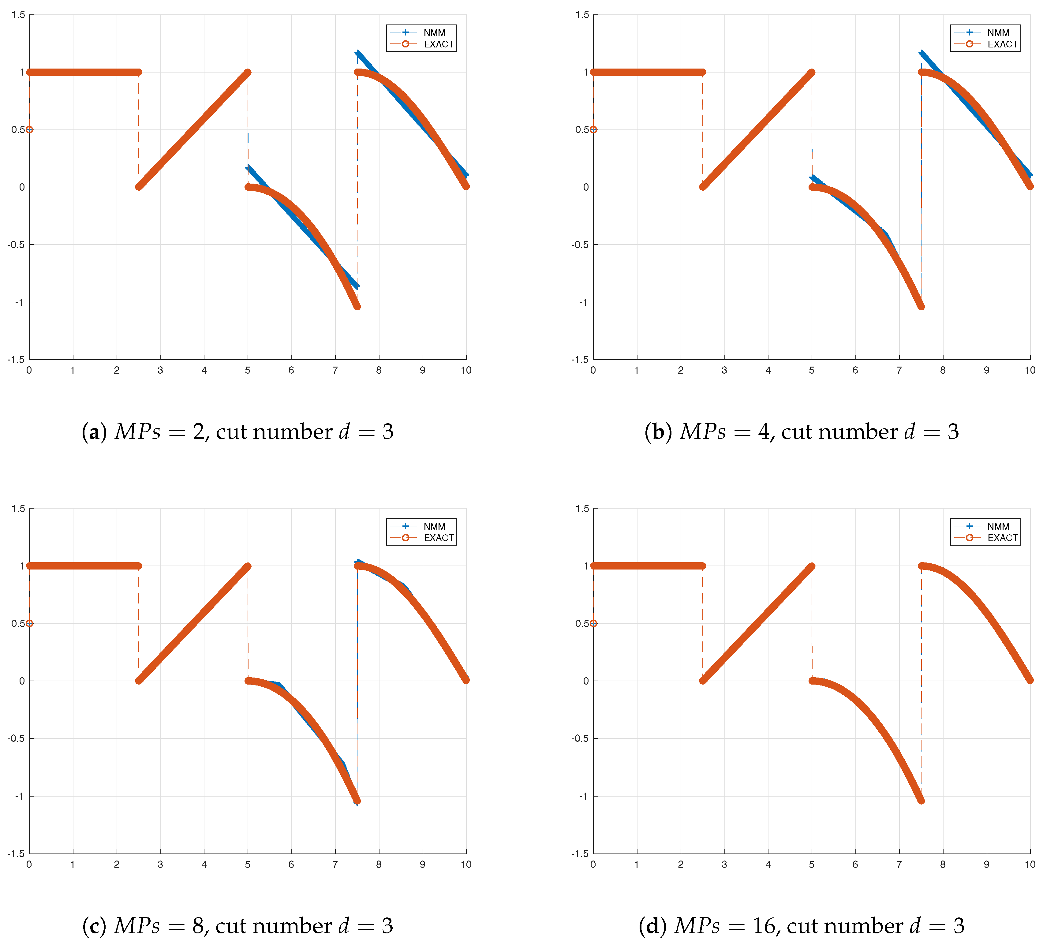
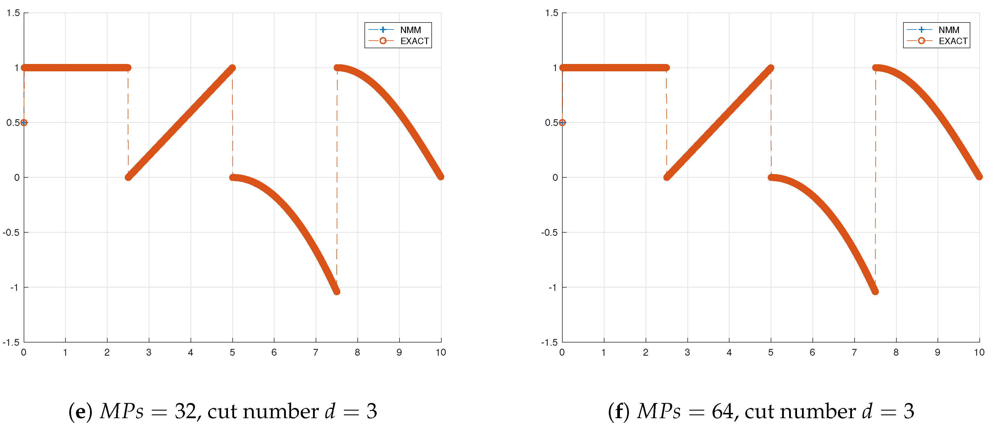
As exhibited in Figure 8 the object function is below according to points number:

$$f\left(x\right)=\left\{\begin{array}{ccc}1\hfill & \hfill & x\in [0,2,5)\hfill \\ \frac{(2x-5)}{5}\hfill & \hfill & x\in [2.5,5)\hfill \\ \frac{{(x-5)}^2}{6}\hfill & \hfill & x\in [5,7.5)\hfill \\ cos\left(\frac{\pi }{5}x-\frac{3\pi }{2}\right)\hfill & \hfill & x\in [7.5,10]\hfill \end{array}\right.$$

(18)

The numbers of mathematical cover are $2,4,8,16,32,64$ as show in Figure 8a–f, and

Table 1. The convergency of NMM with initial mathematical cover, the error is decreasing when the initial MPs is increasing.

MPs Number	Discontinuities Number	PPs Number	Err	lg(Err)
2	3	8	0.05	−1.301029996
4	3	10	0.352	−1.453457337
8	3	14	0.0139	−1.8569852
16	3	22	0.0034	−2.468521083
32	3	38	8.17 × 10−4	−3.087549428
64	3	70	2.01 × 10−4	−3.696587929

summarizes that the error has reduced with the increasement of mathematical cover. Although the initial mathematical cover is less, more physical patches will be generated by cutting the original PPs.

The next examination is to verify the relation between the error and the order of local approximation.

5.3. The Convergency with Higher Order Local Approximation

The object in this example is the same as the previous one. Constant function, polynomial of the first degree, polynomial of the second degree, cosine function, are tested in four parts. If the local approximation is zero order, then the solution will at least approximate the first two part. Meanwhile, the first three functions can be approximated more accurately if the degree of the local Legendre polynomials is one. All the cases above only have two mathematical covers, but the preprocessing produce more physical patches to satisfied the problem domain and the boundary. The related result can be seen in Figure 9a,b, the zero-order case and the first order case, which have error $0.0499$ and $0.0041$ respectively.

5.4. 1D Advection Equations

This example exhibits a linear advection equation:

$$\frac{\partial u}{\partial t}+c\frac{\partial u}{\partial x}=0$$

(19)

When the wave speed $c=1$, the initial condition is

$$f(x,0)=\left\{\begin{array}{cc}\hfill \frac{e^{-{(x-ct-3)}^2}}{10}& x\in [0,3)\hfill \\ \hfill \frac{3e^{-{(x-ct-3)}^2}}{10}& x\in [3,10]\hfill \end{array}\right.$$

(20)

The calculation results are shown in Figure 10a,b. Figure 10a indicates the analytical solution and some general finite volume methods, such as Upwind scheme, Lax Wendroff, Beam Warming, Fromm, Minmod phi, Superbee, MC phi, van Leer, and analytical solution at $t=0.5$, and the discontinuity can be always been maintained by these methods. Figure 10b shows the result of NMM.

We can see that NMM can approximate the exact solution well and has higher accuracy when discontinuity occurs. NMM has successfully shown more flexibility in using analytical solutions such as the speed of shock wave calculated by the Ranking condition.

6. Conclusions

In this paper, a general NMM is developed in general equations with initial discontinuity, where the local approximation is a composition of Legendre polynomials. The hat function is used to construct the PU. We tested NMM using several examples, and there are some conclusions shown as follows:

• NMM can approximate the solution using different local approximation, and the local approximation can be any order.
• The higher order NMM has bigger kernel space with providing better precision.
• NMM can be successfully used to deal with the discontinuity capture, due to the divisible physical patches.
• Although there are discontinuities, the “rank problem” (linear dependence) will not occur when the physical patches are cut. The uniqueness and existence of solution can be verified by numerical examples.
• For dealing with discontinuities, we can cut the physical patches at discontinuities, and add more equations at discontinuities. We can also cover the discontinuity with mathematical patches by using exact solver such as Riemann solver.
• The speed of the discontinuities should be determined by the Ranking condition when discontinuities occur.