Abstract
In this study, a numerical model is proposed for the analysis of a simply supported structural cable. Smoothed particle hydrodynamics (SPH)—a mesh-free, Lagrangian method with advantages for analysis of highly deformable bodies—is utilized to model a cable. In the proposed numerical model, it is assumed that a cable has only longitudinal stiffness in tension. Accordingly, SPH equations derived for solid mechanics are adapted for a structural cable, for the first time. Besides, a proper damping parameter is introduced to capture the behavior of the cable more realistically. In order to validate the proposed numerical model, different experimental and numerical studies available in the literature are used. In addition, novel experiments are carried out. In the experiments, different harmonic motions are applied to a uniformly loaded cable. Results show that the SPH method is an appropriate method to simulate the structural cable.
1. Introduction
Cable is a general name for structural elements with a high ratio of length per diameter. This special geometry makes cables flexible elements in transverse direction. In other words, a cable has almost zero bending stiffness compared to its tension stiffness. It can be formed by many different materials such as steel wires or fibers or a combination of both. These geometric and structural properties make cable indispensable elements for many structures. Cables are widely used in civil engineering structures (e.g., tele skis, prestressing and post-tensioning process, guyed towers, cable stayed bridges, transmission lines, mooring lines) as the main component of them. Therefore, an accurate analysis of cables is very important for safer civil engineering structures.
Analysis of cables has been the interest of many researchers. Different analysis methods have been proposed to simulate highly nonlinear cable elements. The nonlinearity is mostly geometric due to a cable’s structural properties. Nonlinearity of the cable was directly considered in various studies by using the finite element method. For example, a method called a method of imaginary reactions, which considers the geometric nonlinearity, developed by [1]. The same method was also used to solve the issue of a cable having different support conditions in [2]. Besides, closed-form solutions were proposed which consider the nonlinearity of the cable by assuming a deflected shape [3]. For an example of closed-form solutions, the nonlinearity was presupposed with an equivalent Young’s modulus approach [4]. On the other hand, linear shape assumptions were also proposed [5]. This type of solution assumes the cable element is weightless, thus, the cable behaves like a structural bar element. Instead of closed-form solutions and linear approaches, different finite element methods have been proposed. Among the finite element models, a two-node cable element was used in different studies. In [1,2], an initial reaction was assumed to find the geometry of cable and reaction was changed until the boundary condition of the problem, which is the real form of the catenary cable, was satisfied. The authors in [6] carried out geometric nonlinear analysis of cables by using a two-node element with a displacement control method. In [7], a simple two-node straight line cable element was proposed and compared with a multi-node finite element model, which was also the topic of [8]. Besides finite element models including a catenary cable element were also used for dynamic analysis in [9,10]. In addition, two different catenary cable elements, named as continuous and discrete, were proposed [11]. In a further research of Demir [12], finite element method combined with contact mechanics was used to model multi-segment cables which are in contact with a truss system.
Although studies about cables have been mostly performed by mesh-based methods, meshless methods were also used. A solution technique using the element-free Galerkin (EFG) method was proposed for cable reinforced membrane structures [13]. In that study, a penalty method was used to model the sliding between cable and membrane. In [14], an analysis about overhead power line cables was carried out. In the study, a meshless finite difference method (MFDM) was proposed to simulate cables. In another study, Bai and Niedzwecki proposed a meshless method for the model of extensible slender rods which can be regarded as a cable with a small bending stiffness [15]. The method was named as local radial point interpolation method (LRPIM). After the buckling of the column, catenary cable and an entangled cable were solved as validation cases.
Among the meshless methods, smoothed particle hydrodynamics (SPH) is one of the most popular ones. SPH was originally introduced by Lucy [16] and Gingold and Monaghan [17] for astrophysical problems. Subsequently, SPH has been successfully applied to various fields such as open channel [18,19,20] and pipe flows [21], fluid–structure interaction [22,23,24,25], fluid sloshing [26,27,28,29,30], soil mechanics [31], rock mechanics [32] and solid mechanics [33,34,35].
Particle-based methods eliminate the disadvantage of mesh-based methods, which needs mesh regenerations for large deflections and crack propagations, by discretizing the domain with particles. Thus, it is preferred to simulate flows including free surfaces, large deflection problems and crack propagation problems with particle-based methods. As a result of a large deflection problem including rigid body motion due to small transverse stiffness, cables can be considered as a very suitable structural element to be modeled by particle-based methods.
In the present study, the SPH method is implemented with an additional damping term to simulate the dynamic behavior of a structural cable element. As far as the authors’ best knowledge, this is the first study in which a cable is simulated with the SPH method. In addition, a series of novel experiments are conducted for validation purposes. In the experiments, the dynamic response of a cable element under harmonic motion is investigated.
The paper is organized as follows:
- First, the numerical model in which SPH is formulated for the simulation of cable is presented in Section 2.
- The numerical model is validated by comparing the results with different experiments found in the literature in Section 3. Novel experiments conducted for this study are also presented in this section.
- Damping parameters are briefly discussed in Section 4.
- Conclusions are drawn in Section 5.
2. Numerical Model
SPH is a particle-based method, so the continuum is represented by the particles. Using the SPH interpolation, the continuity equation in the Lagrangian approach for the generic particle can be represented as [36,37].
where is the material derivative of the density of th particle, is the mass of th particle, is the velocity difference between particles and and represents the gradient of the kernel function. Kernel function is originally shown by where is the position difference between two neighboring particles and is the smoothing length. In the present study, Wendland C2 kernel with a support domain of 2 is used. is the number of particles and is the speed of the sound. The second term at the right-hand side of the continuity equation is added to remove the numerical oscillations in the pressure field as proposed in [38].
is the diffusive term and the equation is given as:
where is the difference of the position vectors between particles and and is the renormalized density gradient and calculated by
SPH approximation of momentum equation can be represented for each direction as:
where is the Kronecker tensor, is the gravitational acceleration and is the stress tensor and is represented as
where the first term and the second term of the right side are the isotropic and deviatoric parts of the stress tensor, respectively. Pressure, , can be calculated from equation of state in which pressure of a particle is found from the variation of density [39].
where is the bulk modulus of the material. Deviatoric stress can be calculated as:
where is the Young’s modulus and is the rate of transformation vector and calculated as:
is defined for a global coordinate system. In local coordinates of each particle, has only unidirectional strain for a cable model.
In the momentum equation, is the artificial viscosity [40] which is used to reduce the unphysical oscillations in the numerical model.
where and are empirical coefficients taken as 0.2 and 1, respectively.
A damping term denoted as is added into the momentum equation. In this term, is the unstretched cross-sectional area of the cable and is a constant representing the rate of the damping. for each direction can be stated as:
Time is discretized by leap-frog algorithm and maximum step size is calculated from the Courant–Friedrichs–Lewy (CFL) condition [41,42].
3. Validation
To validate the numerical model, different experimental and numerical studies available in the literature are used. In addition, novel experiments are carried out.
3.1. Case 1
A well-known case used in many studies [1,6,10,11,43,44,45,46], is preferred for the statistical validation of the numerical model. Parameters of the model are given in Table 1 and Figure 1.

Table 1.
Parameters used in case 1.
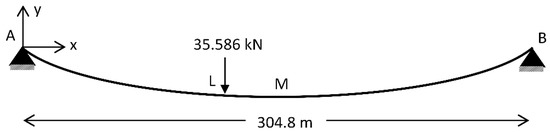
Figure 1.
Model of case 1.
Coordinates of points L and M on a cable under catenary action are (121.92 m, −29.276 m) and (152.4 m, −30.48 m), respectively. An external load 35.586 kN is applied at point L of the cable after taking its catenary form under self-weight. Displacement of point L after the application of external load is used as the validation parameter in the literature.
For the numerical model, the number of particles is found to be 312 after a convergence test. The cable is initially defined as linear and the right support is initially located at 0 m and 312.73 m. By moving the right support to its original position (0 m, 304.80 m), the cable is allowed to sag to its natural catenary form. After oscillations vanish and the cable reaches its final form under self-weight, the external point load shown in Figure 1 is applied at point L. Figure 2 shows the time history of the positions of L in y direction. External load is applied at the 150th second when the oscillations completely vanish. Final displacement of point L can be seen in Table 2. According to the table, calculated final displacement of point L is consistent with the data in the literature. Since the support is moved instantly at the beginning of the simulation, the initial oscillations are very high as can be seen in Figure 2. High initial oscillations may be avoided by defining the initial configuration of the particles similar to the natural catenary form of the cable. However, the oscillations do not create a convergence problem. In addition, they completely vanish thanks to the damping parameter proposed in the present study.
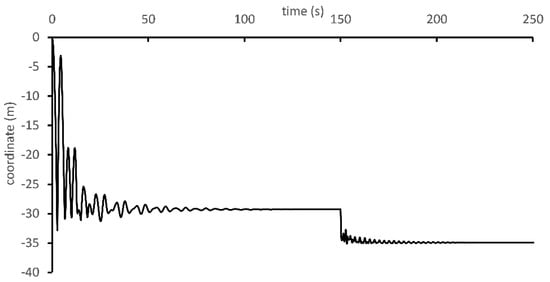
Figure 2.
Time history of coordinate of point L in y direction.
Table 2.
Final displacement of point L.
3.2. Case 2
An experiment from the literature [9], in which free vibration of a suspended cable was investigated, is used to validate the numerical model dynamically. The experimental setup is given in Figure 3 and parameters of model are given in Table 3. After instant removal of additional mass defined at the midpoint of the cable, the displacement of the same point is measured.
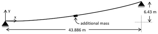
Figure 3.
Model of case 2.
Table 3.
Parameters used in case 2.
The number of particles used to simulate the experiments is 44, as obtained from a convergence test. The second support coordinate is defined at 43.835 m and 6.43 m initially, and the cable is defined between these supports linearly. The second support is relocated to its original position shown in Figure 3. The cable takes its catenary form under its self-weight and the additional mass. Then, mass is removed, and time history of midpoint displacement is calculated.
The displacement history of the free vibration at the midpoint of the cable is given in Figure 4. In the figure, the experimental and numerical data in [9] and the present numerical results labeled as SPH are shown. The first peak is slightly overestimated by the SPH method. Other peaks are predicted satisfactorily.
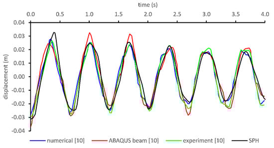
Figure 4.
Displacement in y direction at the midpoint of a suspended catenary cable in Case 2.
3.3. Experiment
In addition to the verification cases procured from the previous studies, an experimental study available in the literature is repeated, and a novel benchmark experiment is designed in the context of this study. In both experiments, the same cable was used which is specifically designed to validate the particle-based methods. In the design of the experimental setup, spherical weights were placed throughout the cable with the same intervals. The distance between each spherical weight was designed as 2.6 mm to satisfy the assumption that adjacent spherical weights do not contact with each other during the dynamic motion of the cable. Center-to-center distance between adjacent spherical weights was 10.6 mm and each sphere had a mass of 0.285 g including the mass of cable. Thus, the cable model had a 0.2656 N/m self-weight. Bending stiffness of the cable was assumed to be zero. A uniformly loaded cable model designed in accordance with the particle-based models was achieved. Tensile modulus of the cable was recorded as 109 GPa.
A high-definition camera was used to digitize the motion of the cable with the help of an image processing technique. The camera can capture 60 frames per second with 720 pixels. Some intermediate spherical weights on the cable were marked and their motions were recorded and digitized.
3.3.1. Experiment 1
This experiment is inspired by the experiments available in the literature. It was first presented by [47], used in [48] and repeated in the study of [49]. It is a basic experiment for the investigation of dynamic motion of cables. In the previous versions of this experiment, the cable was released from the support of a catenary position defined in Figure 5 and the dynamic motion of it was supplied via camera. Snapshots from a camera were given. No additional numerical data were presented.
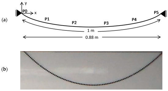
Figure 5.
Initial geometry of the cable in experiment 1 of (a) schematic view and (b) real image.
In the research of [47], experimental data were supplied by using the recorded snapshots via camera. However, cable positions were not given in equally spaced time intervals [47]. A numerical solution was also presented with given time intervals. In [48], the experimental data supplied by [47] was used to verify the cable model. Positions of a free-falling cable for specified time intervals were presented as numerical results of that research. The experiment of Fried [47] was repeated in [49]. In that study, configuration of the cable was compared with the experimental snapshots. In this research, time intervals of numerical analysis were supplied, however time instants of experimental snapshots were not presented.
A brief discussion of numerical methods used to simulate the free-falling cable is given as follows. In the research of Coyette and Guisset [48], the finite element method was used with the following assumptions: cables possess only axial stiffness, material is linearly elastic and only small strains are involved. The same assumptions were used in the finite element model of Fried [47] which was called a chain model. Lazzari et al. [49] also used the finite element method for the cable and Akaike-Iwatani model [50] for wind effect on cable. Notably, none of these studies included the damping effect in their finite element model. Similar to the previous studies conducted with the finite element method, SPH equations are derived with the same assumptions. Since a cable has no stiffness in its transverse direction, either singularity of stiffness matrix or high displacements can be observed. This is the main drawback of finite element models. Proper algorithms should be proposed to deal with this problem as in [6]. The nature of SPH minimizes this type of problem.
Initial geometry of the cable was defined as in previous studies mentioned above. A cable with a 1 m length was supported at its ends as illustrated in Figure 5. Supports were placed at the same elevation, and the distance between the supports in x direction was defined as 0.88 m. The cable is supported at end points, P0 and P5. A cable with 95 spherical weights was suspended as defined in Figure 5 and released from P5. Intermediate points were defined through the geometry of the cable with the cable length measured from P0 as given in Table 4 where P5 is the free end.
Table 4.
Positions of intermediate points of cable in experiment 1.
The experiment was repeated in the context of this research to digitize the motion of the cable in detail. Accordingly, the displacements of specified intermediate points throughout the cable are supplied. The main contribution of this experiment is to give the digitized time history of a free-falling cable.
In the numerical model, 95 particles were used. Due to the Lagrangian nature of the SPH method, the positions of all the particles were followed. Therefore, the number of particles used in the simulations was taken to be the same as the number of spherical weights, although a convergence analysis was performed and according to the convergence analysis it was found that less particles can be used. Convergence analysis results are given for the following experiment.
Figure 6 and Figure 7 show the displacement of intermediate points and the free end. The simulated displacements of intermediate points are close to the experimental data. However, the displacement of the free end is slightly overestimated in SPH. The reason for this slight difference is the particle approximation and kernel integration errors at the free end of the cable.
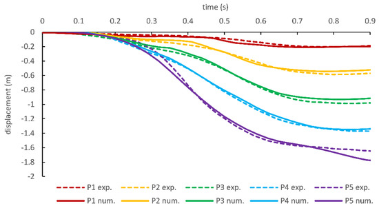
Figure 6.
Displacement in x coordinates of internal points on cable.
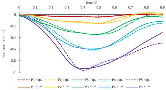
Figure 7.
Displacement in y coordinates of intermediate points on cable.
Displacement of P5 (free-end) is compared with the literature data in Figure 8 and Figure 9 (comparison of displacement of intermediate points is not possible due to the lack of reproducibility of previous studies). As mentioned above, time intervals were not clearly stated for the experiments available in the literature, thus numerical data were compared qualitatively. Previous numerical data available in the literature are scaled with respect to time based on the experiment carried out in this study for a quantitative comparison. It should be mentioned that scale factor is constant for each study. According to the figure, it can be said that SPH can predict the dynamic motion of the cable reasonably well.
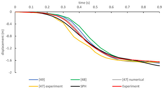
Figure 8.
Comparison of free-end displacement in x direction.
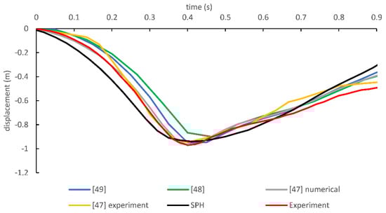
Figure 9.
Comparison of free-end displacement in y direction.
3.3.2. Experiment 2
The second experiment is a novel setup designed in the context of this study for dynamic verification of the proposed numerical method. A cable with a 1.272 m length was supported at its ends as illustrated in Figure 10. The distances between the supports in x and y directions were 1.2 m and 0.22 m, respectively.
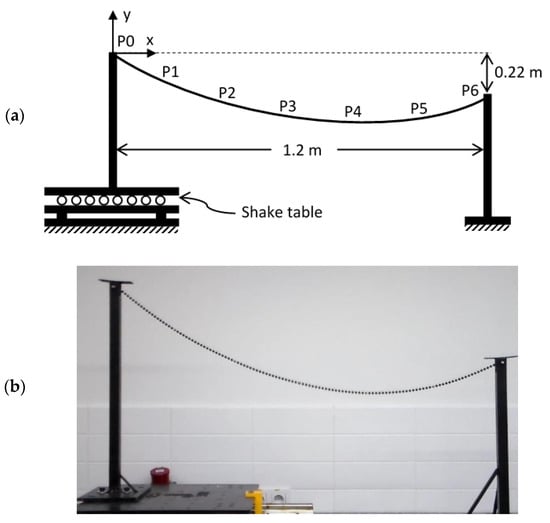
Figure 10.
Setup of experiment 2 of (a) schematic view and (b) real image.
P6 was fixed on the ground while P0 was fixed on a shake table which has a motion in the x-direction. The cable was suspended between these supports and a catenary shape was formed. Coordinates of the initial catenary shape of the cable are given in Table 5. After achieving a stationary catenary shape, two different excitations with the same amplitude of 25 mm and with frequencies of 1.0 and 1.5 Hz were applied to P0 via the shake table. These harmonic motions are referred to as Type1 and Type2, for frequencies 1.0 and 1.5 Hz, respectively.
Table 5.
Positions of intermediate points of cable in experiment 2.
The displacement in y direction of P3 was used for convergence analysis. The number of particles was defined as being 2 times the number of spherical weights and half of it. Analyses were repeated for both motion types as seen in Figure 11. Although no significant difference is observed for different numbers of particles for Type1, a noise is seen at about 2.5 s and 4.5 s for Type2. The noise exists for a greater number of particles (121 and 242). Nevertheless, a further analysis was carried out by increasing the number of particles (482). This same noise still occurs, so the number of particles is enough for the convergence analysis. For a greater number of particles, some particles in numerical analysis were in a position where no mass was defined in the experimental setup. Nevertheless, convergence parameter shows similar results for a greater number of particles than 61. In all the simulations, the number of 121 particles was preferred, because each spherical weight in the experiments was represented by an SPH particle.
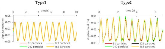
Figure 11.
Convergence analysis results for both motion types.
The simulated and measured displacement history of the defined points can be seen in Figure 12 and Figure 13 for Type1 and Type2, respectively. In the figures, black and red continuous lines show the experimental and numerical data, respectively. Due to the harmonic excitations, the cable started to displace. The simulated excitation-driven motion of the cable perfectly matches with the experimental data in terms of the period and amplitude.
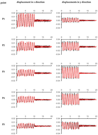
Figure 12.
Numerical (red) and experimental (black) comparison of time (s) (horizontal axis) vs. displacement (m) (vertical axis) graph of specified nodes on cable under harmonic motion Type1.
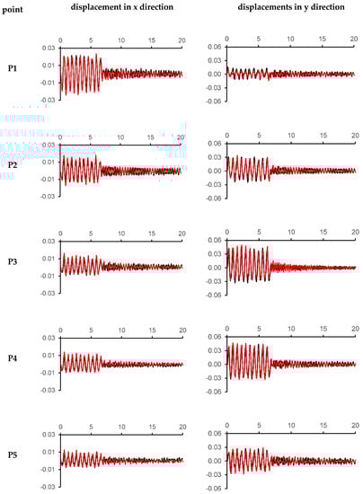
Figure 13.
Numerical (red) and experimental (black) comparison of time (s) (horizontal axis) vs. displacement (m) (vertical axis) graph of specified nodes on cable under harmonic motion Type2.
After the end of excitation-driven motion, oscillations start. The oscillations should end after a while due to friction and damping. A damping term was added to the numerical model for a gradual decrease in oscillations. As expected, numerical oscillations were more regular than experimental ones. Besides, the periods of oscillations were the same for both harmonic motions (Type1 and Type2); it was 0.45 s for numerical analysis and 0.42 s for experimental investigations. Although a perfect match was obtained in the excitation-driven part of the motion of cable, there was a slight difference in the oscillations part as indicated.
Additionally, reactions in x and y directions for each support at P0 and P6 are given in Figure 14. There are two verification conditions for a cable in static catenary form. First, the magnitude of reactions in x directions of both supports must be equal for any cable in its catenary action. This condition is verified for both harmonic motions, as seen in Figure 14. Second, the summation of magnitude of reactions in y direction of both supports must be equal to the weight of the hanging cable. In this experiment, the summation was 0.338 N which was equal to the total weight of the cable.
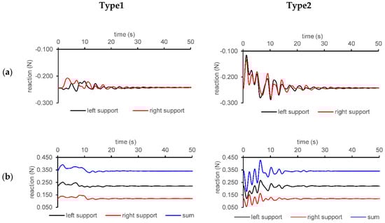
Figure 14.
Time history of magnitudes of reactions on supports in (a) x and (b) y direction.
4. Discussion on Damping Parameter
The dynamic motion of a disturbed cable continues without damping even after the removal of external loads. Therefore, a damping parameter is defined in the proposed method to mimic the nature of the dynamic behavior of a cable. In the well-known governing equation of the motion of solids, there is a damping contribution which is achieved by multiplication of the velocity with damping matrix. Rayleigh damping [51] is widely used to determine a damping matrix. In that method, the damping matrix is preferably defined with the mass and/or stiffness matrix [52,53,54]. In the proposed method, the mass of particles is used to define a damping for the motion. Accordingly, mass times velocity term is defined to model the damping effect, as seen in Equation (12).
As seen in Figure 15, the disturbed cable oscillates after the end of harmonic motion applied by the shake table. The amplitude and period of these oscillations are different from the experimental results. After application of the damping term, closer results to the experimental data were achieved. As shown in Figure 15, the excitation-driven part of the motion is not significantly affected by the damping term. This damping term consists of a problem-dependent parameter, , as shown in Equation (5) as in the Rayleigh damping method. There have been studies that sought to define the constants of the Rayleigh method experimentally and analytically. Yaqiang et al. [55] determined Rayleigh constants for some fiber-reinforced polymer (FRP) cables experimentally. Maji and Qiu [56,57] also carried out experiments for measuring and understanding the damping characteristics of a cable. In addition, Zhu and Meguid [58] studied the damping behavior of a cable, especially on 6 × 37 IWRC (independent wire rope core), experimentally and analytically. In all studies, damping parameters were either determined for special cable products experimentally or by an estimation made analytically as mentioned in [59]. Rayleigh constants can also be estimated numerically by modal analysis which is often made by the finite element method. However, there is no modal analysis made by the SPH method. Authors prefer to assume the damping parameter,, is between 0.03 and 0.05 which satisfies the consistent damping rate observed in the experiments and leave the broad damping concept for further research.
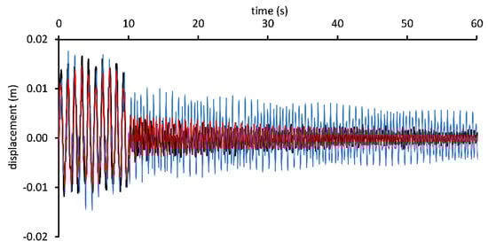
Figure 15.
Displacement of P1 under Type1 excitation for experiment (black) and numerical solution without damping (blue) and with damping (= 0.04) (red).
5. Conclusions and Future Works
In this paper, a numerical model is proposed to simulate the dynamic motion of a structural cable. In the numerical model, SPH is used. First, the numerical model was validated with for the case of which static solutions were available. Then, another case was used to validate the model under dynamic motion. Although, there are many problems available in the literature in validating the model, such approaches are limited in showing the real capability of the proposed numerical method. For example, the results of experiments in the literature were presented only for a limited time, or the displacement of only one point on the cable was presented. For these reasons, novel experiments were conducted. The main contribution of the experiments is to present the displacement of the whole cable profile by giving the displacement history of intermediate points on the cable. In addition, an extended time history analysis is provided to investigate the dynamic motion of the cable which does not end for a long time after the excitation vanishes.
In the numerical model, a proper damping parameter is proposed. Damping becomes effective when the excitations are removed. Therefore, the results while the excitation is still applied are very similar, independent of the damping. However, oscillations observed in the experiments after the excitation ends cannot be captured in the numerical model without a proper damping parameter. After the addition of the damping parameter, results closer to the experimental data were obtained. To the best of the authors’ knowledge, this is the first study that investigates the damping effect of the cable.
Although validations show that SPH, with a proper damping parameter, can be used to model the dynamic motion of the cable satisfactorily, there are some limitations of the numerical model. The limits of the damping parameter should be investigated in detail. Since more computational study should be performed and new experiments should be carried out to investigate the effect of damping parameters appropriately, it is left for a future study. In addition, the current version of the proposed numerical model can simulate the single-segment cables. Another future work will be focused on the application of the numerical model for multi-segment cables which includes additional intermediate roller supports or pulleys resulting in a frictional force to be modeled.
Author Contributions
Investigation, A.E.D. and A.D.; Methodology, A.D.; Software, A.E.D.; Validation, A.E.D. and A.D.; Writing—original draft, A.E.D. and A.D. Revision, A.E.D. and A.D. All authors have read and agreed to the published version of the manuscript.
Funding
This research received no external funding.
Conflicts of Interest
The authors declare no conflict of interest.
References
- Michalos, J.; Birnstiel, C. Movements of a cable due to changes in loading. Trans. Am. Soc. Civ. Eng. 1962, 127, 267–281. [Google Scholar]
- Demir, A. Form Finding and Structural Analysis of Cables with Multiple Supports. Master’s Thesis, Middle East Technical University, Ankara, Turkey, 2011. [Google Scholar]
- Ernst, H.J. Der E-Modul von Seilen unter Brucksichtigung des Durchhangers. Der Bauing. 1965, 40, 52–55. [Google Scholar]
- Liew, J.Y.R.; Punniyakotty, N.M.; Shanmugam, N.E. Limit-State Analysis and Design of Cable-Tensioned Structures. Int. J. Space Struct. 2001, 16, 95–110. [Google Scholar] [CrossRef]
- Cleary, P.W.; Rudman, M. Extreme wave interaction with a floating oil rig: Prediction using SPH. Prog. Comput. Fluid Dyn. 2009, 9, 332–344. [Google Scholar] [CrossRef]
- Yang, Y.B.; Tsay, J.-Y. Geometric nonlinear analysis of cable structures with a two-node cable element by generalized displacement control method. Int. J. Struct. Stab. Dyn. 2007, 7, 571–588. [Google Scholar] [CrossRef]
- Chunjiang, W.; Renpeng, W.; Shilin, D.; Ruojun, Q.; Wang, C.; Wang, R.; Dong, S.; Qian, R. A New Catenary Cable Element. Int. J. Space Struct. 2003, 18, 269–275. [Google Scholar] [CrossRef]
- Chen, Z.H.; Wu, Y.J.; Yin, Y.; Shan, C. Formulation and application of multi-node sliding cable element for the analysis of Suspen-Dome structures. Finite Elem. Anal. Des. 2010, 46, 743–750. [Google Scholar] [CrossRef]
- Chang, S.-P.; Park, J.-I.; Lee, K.-C. Nonlinear dynamic analysis of spatially suspended elastic catenary cable with finite element method. KSCE J. Civ. Eng. 2008, 12, 121–128. [Google Scholar] [CrossRef]
- Thai, H.-T.T.; Kim, S.-E.E. Nonlinear static and dynamic analysis of cable structures. Finite Elem. Anal. Des. 2011, 47, 237–246. [Google Scholar] [CrossRef]
- Salehi, A.A.M.; Shooshtari, A.; Esmaeili, V.; Naghavi Riabi, A. Nonlinear analysis of cable structures under general loadings. Finite Elem. Anal. Des. 2013, 73, 11–19. [Google Scholar] [CrossRef]
- Demir, A. Multi-Segment Continuous Cables with Frictional Contact Along Their Span. Ph.D. Thesis, Middle East Technical University, Ankara, Turkey, 2017. [Google Scholar]
- Noguchi, H.; Kawashima, T. Meshfree analyses of cable-reinforced membrane structures by ALE–EFG method. Eng. Anal. Bound. Elem. 2004, 28, 443–451. [Google Scholar] [CrossRef]
- Cecot, W.; Milewski, S.; Orkisz, J. Determination of Overhead Power Line Cables Configuration by FEM and Meshless FDM. Int. J. Comput. Methods 2018, 15. [Google Scholar] [CrossRef]
- Bai, Y.; Niedzwecki, J.M. Meshfree analysis of structures modeled as extensible slender rods. Eng. Struct. 2018. [Google Scholar] [CrossRef]
- Lucy, L.B. A numerical approach to the testing of the fission hypothesis. Astron. J. 1977, 82, 1013–1024. [Google Scholar] [CrossRef]
- Gingold, R.A.; Monaghan, J.J. Smoothed particle hydrodynamics: Theory and application to non-spherical stars. Mon. Not. R. Astr. Soc. 1977, 181, 375–389. [Google Scholar] [CrossRef]
- Gu, S.; Bo, F.; Luo, M.; Kazemi, E.; Zhang, Y.; Wei, J. SPH simulation of hydraulic jump on corrugated riverbeds. Appl. Sci. 2019, 9, 436. [Google Scholar] [CrossRef]
- Shu, A.; Wang, S.; Rubinato, M.; Wang, M.; Qin, J.; Zhu, F. Numerical modeling of debris flows induced by dam-break using the smoothed particle hydrodynamics (SPH) method. Appl. Sci. 2020, 10, 2954. [Google Scholar] [CrossRef]
- Zheng, X.; Ma, Q.; Shao, S. Study on SPH viscosity term formulations. Appl. Sci. 2018, 8, 249. [Google Scholar] [CrossRef]
- Hou, D.Q.; Tijsseling, A.S.; Bozkus, Z. Dynamic force on an elbow caused by a traveling liquid slug. J. Press. Vessel Technol. Trans. ASME 2014, 136. [Google Scholar] [CrossRef]
- Demir, A.; Dinçer, A.E. MPS ve FEM Tabanlı Akışkan-Yapı Etkileşimi Modelinin Çoruh Nehri Üzerindeki Ardıl Baraj-Yıkılma Problemine Uygulanması. Doğal Afetler ve Çevre Dergisi 2017, 3, 64–69. [Google Scholar] [CrossRef]
- Demir, A.; Dinçer, A.E.; Bozkus, Z.; Tijsseling, A.S. Numerical and experimental investigation of damping in a dam-break problem with fluid-structure interaction. J. Zhejiang Univ. Sci. A 2019, 20, 258–271. [Google Scholar] [CrossRef]
- Dinçer, A.E.; Demir, A.; Yavuz, C. A Preliminary study for fluid structure interaction model by smoothed particle hydrodynamics and contact mechanics. In Proceedings of the 37th IAHR World Congress, Kuala Lumpur, Malaysia, 13–18 August 2017. [Google Scholar]
- Dinçer, A.E.; Demir, A.; Bozkus, Z.; Tijsseling, A.S. Fully Coupled Smoothed Particle Hydrodynamics-Finite Element Method Approach for Fluid-Structure Interaction Problems With Large Deflections. J. Fluids Eng. Trans. ASME 2019, 141, 081402. [Google Scholar] [CrossRef]
- Dinçer, A.E. Investigation of the Sloshing Behavior Due to Seismic Excitations Considering Two-Way Coupling of the Fluid and the Structure. Water 2019, 11, 2664. [Google Scholar] [CrossRef]
- Dinçer, A.E. Experimental and numerical investigation of hyper-elastic submerged structures strengthened with cable under seismic excitations. Eur. J. Environ. Civ. Eng. 2020, 1–20. [Google Scholar] [CrossRef]
- Demir, A. Hydro-elastic analysis of standing submerged structures under seismic excitations with SPH-FEM approach. Lat. Am. J. Solids Struct. 2020, 17. [Google Scholar] [CrossRef]
- Zhao, Y.; Li, H.-N.; Zhang, S.; Mercan, O.; Zhang, C. Seismic Analysis of a Large LNG Tank Considering Different Site Conditions. Appl. Sci. 2020, 10, 8121. [Google Scholar] [CrossRef]
- Zheng, X.; You, Y.; Ma, Q.; Khayyer, A.; Shao, S. A comparative study on violent sloshing with complex baffles using the ISPH method. Appl. Sci. 2018, 8, 904. [Google Scholar] [CrossRef]
- Nonoyama, H.; Moriguchi, S.; Sawada, K.; Yashima, A. Slope stability analysis using smoothed particle hydrodynamics (SPH) method. Soils Found. 2015, 55, 458–470. [Google Scholar] [CrossRef]
- Niroumand, H.; Mehrizi, M.E.M.; Saaly, M. Application of SPH Method in Simulation of Failure of Soil and Rocks Exposed to Great Pressure. Soil Mech. Found. Eng. 2017, 54, 216–223. [Google Scholar] [CrossRef]
- Antoci, C.; Gallati, M.; Sibilla, S. Numerical simulation of fluid-structure interaction by SPH. Comput. Struct. 2007, 85, 879–890. [Google Scholar] [CrossRef]
- Shutov, A.; Klyuchantsev, V. On the application of SPH to solid mechanics. J. Phys. Conf. Ser. 2019, 1268, 012077. [Google Scholar] [CrossRef]
- Limido, J.; Espinosa, C.; Salaün, M.; Lacome, J.L. SPH method applied to high speed cutting modelling. Int. J. Mech. Sci. 2007, 49, 898–908. [Google Scholar] [CrossRef]
- Dinçer, A.E. Numerical Investigation of Free Surface and Pipe Flow Problems by Smoothed Particle Hydrodynamics. Ph.D. Thesis, Middle East Technical University, Ankara, Turkey, 2017. [Google Scholar]
- Dinçer, A.E.; Bozkuş, Z.; Tijsseling, A.S. Prediction of Pressure Variation at an Elbow Subsequent to a Liquid Slug Impact by Using Smoothed Particle Hydrodynamics. J. Press. Vessel Technol. Trans. ASME 2018, 140. [Google Scholar] [CrossRef]
- Marrone, S.; Antuono, M.; Colagrossi, A.; Colicchio, G.; Le Touzé, D.; Graziani, G. δ-SPH model for simulating violent impact flows. Comput. Methods Appl. Mech. Eng. 2011, 200, 1526–1542. [Google Scholar] [CrossRef]
- Monaghan, J.J. Simulating Free Surface Flows with SPH. J. Comput. Phys. 1994, 110, 399–406. [Google Scholar] [CrossRef]
- Liu, G.R.G.; Liu, M.B. Smoothed Particle Hydrodynamics: A Mesh-Free Particle Method, 1st ed.; World Scientific Publishing Co. Pte. Ltd.: Singapore, 2003; ISBN 981-238-456-1. [Google Scholar]
- Anderson, J.D. Computational Fluid Dynamics: The Basics with Applications; McGraw-Hill: New York, NY, USA, 1995. [Google Scholar]
- Hirsch, C. Numerical Computation of Internal and External Flows: The Fundamentals of Computational Fluid Dynamics; Elsevier: Amsterdam, The Netherlands, 2007; ISBN 9780750665940. [Google Scholar]
- Andreu, A.; Gil, L.; Roca, P. A new deformable catenary element for the analysis of cable net structures. Comput. Struct. 2006, 84, 1882–1890. [Google Scholar] [CrossRef]
- Jayaraman, H.B.; Knudson, W.C. A curved element for the analysis of cabe structures. Trans. Am. Soc. Civ. Eng. 1962, 127, 267–281. [Google Scholar]
- O’Brien, W.T.; Francis, A.J. Cable movements under two-dimensional loads. J. Struct. Div. ASME 1964, 90, 89–124. [Google Scholar]
- Tibert, G. Numerical Analyses of Cable Roof Structures; KTH: Stockholm, Sweden, 1999. [Google Scholar]
- Fried, I. Large deformation static and dynamic finite element analysis of extensible cables. Comput. Struct. 1982, 15, 315–319. [Google Scholar] [CrossRef]
- Coyette, J.P.; Guisset, P. Cable network analysis by a nonlinear programming technique. Eng. Struct. 1988, 10, 41–46. [Google Scholar] [CrossRef]
- Lazzari, M.; Saetta, A.V.; Vitaliani, R.V. Non-linear dynamic analysis of cable-suspended structures subjected to wind actions. Comput. Struct. 2001, 79, 953–969. [Google Scholar] [CrossRef]
- Iwatani, Y. Simulation of multidimensional wind fluctuations having any arbitrary power spectra and cross-spectra. J. Wind Eng. 1982, 11, 5–18. [Google Scholar] [CrossRef]
- Song, Z.; Su, C. Computation of Rayleigh Damping Coefficients for the Seismic Analysis of a Hydro-Powerhouse. Shock Vib. 2017, 2017, 2046345. [Google Scholar] [CrossRef]
- Liu, M.; Gorman, D.G. Formulation of Rayleigh damping and its extensions. Comput. Struct. 1995, 57, 277–285. [Google Scholar] [CrossRef]
- Hall, J.F. Problems encountered from the use (or misuse) of Rayleigh damping. Earthq. Eng. Struct. Dyn. 2006, 35, 525–545. [Google Scholar] [CrossRef]
- Kazaz, İ. Seismic deformation demands on rectangular structural walls in frame-wall systems. Earthq. Struct. 2016, 10, 329–350. [Google Scholar] [CrossRef]
- Yaqiang, Y.; Xin, W.; Zhishen, W. Experimental Study of Vibration Characteristics of FRP Cables for Long-Span Cable-Stayed Bridges. J. Bridg. Eng. 2015, 20, 4014074. [Google Scholar] [CrossRef]
- Maji, A.; Qiu, Y. Experimental Study of Cable Vibration Damping BT—Dynamic Behavior of Materials; Proulx, T., Ed.; Springer: New York, NY, USA, 2011; Volume 1, pp. 329–336. [Google Scholar]
- Maji, A.K.; Qiu, Y.Z. Experimental and Numerical Investigation of Axially Preloaded Carbon Fiber Cable Vibration. J. Aerosp. Eng. 2014, 27, 4014010. [Google Scholar] [CrossRef]
- Zhu, Z.H.; Meguid, S.A. Nonlinear FE-based investigation of flexural damping of slacking wire cables. Int. J. Solids Struct. 2007, 44, 5122–5132. [Google Scholar] [CrossRef]
- Yang, Y.; Fahmy, M.F.M.; Pan, Z.; Guan, S.; Zhan, Y. Analytical estimation on damping behaviors of the Self-Damping fiber reinforced polymer (FRP) cable. Structures 2020, 25, 774–784. [Google Scholar] [CrossRef]
Publisher’s Note: MDPI stays neutral with regard to jurisdictional claims in published maps and institutional affiliations. |
© 2020 by the authors. Licensee MDPI, Basel, Switzerland. This article is an open access article distributed under the terms and conditions of the Creative Commons Attribution (CC BY) license (http://creativecommons.org/licenses/by/4.0/).