Article

Using BiLSTM Networks for Context-Aware Deep Sensitivity Labelling on Conversational Data

by
Antreas Pogiatzis
* and
Georgios Samakovitis
*
School of Computing and Mathematical Sciences, University of Greenwich, Old Royal Naval College, Park Row, Greenwich, London SE10 9LS, UK
*
Authors to whom correspondence should be addressed.
Appl. Sci. 2020, 10(24), 8924; https://doi.org/10.3390/app10248924
Submission received: 31 October 2020 / Revised: 2 December 2020 / Accepted: 8 December 2020 / Published: 14 December 2020
(This article belongs to the Special Issue Applied Machine Learning)

Abstract

:
Information privacy is a critical design feature for any exchange system, with privacy-preserving applications requiring, most of the time, the identification and labelling of sensitive information. However, privacy and the concept of “sensitive information” are extremely elusive terms, as they are heavily dependent upon the context they are conveyed in. To accommodate such specificity, we first introduce a taxonomy of four context classes to categorise relationships of terms with their textual surroundings by meaning, interaction, precedence, and preference. We then propose a predictive context-aware model based on a Bidirectional Long Short Term Memory network with Conditional Random Fields (BiLSTM + CRF) to identify and label sensitive information in conversational data (multi-class sensitivity labelling). We train our model on a synthetic annotated dataset of real-world conversational data categorised in 13 sensitivity classes that we derive from the P3P standard. We parameterise and run a series of experiments featuring word and character embeddings and introduce a set of auxiliary features to improve model performance. Our results demonstrate that the BiLSTM + CRF model architecture with BERT embeddings and WordShape features is the most effective (F1 score 96.73%). Evaluation of the model is conducted under both temporal and semantic contexts, achieving a 76.33% F1 score on unseen data and outperforms Google’s Data Loss Prevention (DLP) system on sensitivity labelling tasks.

1. Introduction

Diminishing information privacy in communication ecosystems often requires consumers to directly manage their own preferences. Yet, this easily becomes a tedious task considering the amount of information exchanged on a daily basis. Research indicates that, most often, consumers lack the information to take appropriate privacy-aware decisions [1], and even where sufficient information is available, long-term privacy is traded-off for short-term benefits [2] (indicatively, a Facebook-focused empirical user study pointed out that 20% of participants and 50% of interviewees reported direct regret after posting sensitive information publicly) [3]. Automatically identifying sensitive information is critical for privacy-preserving technologies. Sensitive data most often appear as unstructured text, making it vulnerable to privacy threats, due to its parseable and searchable format. This work solely concentrates on text data.
The sensitivity of a piece of information is directly shaped by the context it is provided in. For the purposes of this analysis, we offer a taxonomy of four distinct context classes, for use as sensitivity categories. We derive these respectively by the meaning, interaction, precedence, and preference associated with any piece of information:
Semantic Context: formed on the basis of the semantic meaning of a term. As, for instance, in the case of homonyms or homographs, the semantic meaning of a sequence affects its sensitivity.
Agent Context: depending upon the agents participating in the transmission of information. Here, the relationship between participating actors determines sensitivity. For instance, patient–doctor sharing of medical history is non-sensitive for this set of actors, but sensitive otherwise.
Temporal Context: defined by information precedence that affects the significance of a term. Here, previously introduced definitions of a term qualify its sensitivity. If, for example, a string sequence is introduced as a password, it carries higher sensitivity than if it was introduced as a username.
Self Context: defined by the user’s personal privacy preferences. Notably, what is considered private varies across users due to cultural influences, personal experiences, professional statute, etc. For example, ethnic origin may be considered sensitive information for one individual but not for another.
The above list of context classes is not exhaustive, nor are these mutually exclusive. One or more contexts may simultaneously influence sensitivity differently. Information may, however, be sensitive, regardless of context (e.g., credit-card numbers, email, passwords, insurance numbers). In this work, we use sensitive information as any coherent sequence of textual data from which a third party can elicit information that falls under the categories proposed in the P3P standard (Table 1).
This paper proposes a context-aware predictive deep learning model that can annotate sensitive tokens in a sequence of text data, more formally defined as a “token sensitivity labelling” task. We develop our models for semantic and temporal contexts, as this provides an adequate proof-of-concept, and as incorporating all four contexts requires extraneous methodologies, which are planned for future work. We reduce the problem of sensitivity annotation to a multi-class classification problem and follow deep learning techniques that were proven effective in similar labelling tasks, such as Named Entity Recognition (NER) and Part-of-Speech (POS) tagging [5,6,7]. We develop a context-aware classifier based on the BiLSTM + CRF architecture with word embeddings and WordShape as features. We address dataset limitations by developing data generation algorithms to combine synthetic and real data, and experimentally identify the best performing model architecture and feature combination. The models are first evaluated on a dataset generated with the assistance of synthetic sensitive data, reaching an F1 score of 96.73%. We evaluate our model in two settings: (i) one addressing sensitive information annotation under the influence of temporal context and; (ii) one comparing against Google’s DLP system with semantic context variations. In the former our model reaches an F1 score of 76.33%, and in the latter, results highlight the resiliency of our system on semantic noise by outperforming Google’s DLP in all sensitive information type annotation. We summarise the key contribution of this work as:
  • The introduction of the four context classes (Semantic, Agent, Temporal, Self) as a taxonomy to suitably represent the relationship between candidate sensitive tokens and their textual surroundings (sentence or wider textual sequence). In addition to allowing for context differentiation (for instance, depending on the nature of privacy settings), the taxonomy may be used as a framework for applying sensitivity tiers (for instance by overlaying different types of context-awareness depending on the strictness of privacy settings).
  • The use of BiLSTM-CRF multi-class annotation of sensitive tokens in a context-aware manner, (an approach that, to the best of our knowledge has scarce representation in the literature), the implementation of which outperforms an industry-strength system in sensitivity labelling along at least one context class. (More specifically, our approach differentiates from normal NER (Named-Entity Recognition) tagging in two ways: (a) Although it is technically still a sequence labelling task, it is fundamentally different in the same way that CWI (Complex Word Identification) tagging differs from NER. Our sensitivity labelling is context-aware whereas NER is not. (b) Our work includes a data generation strategy, something that would not be needed in the case of NER).
  • A dataset enrichment methodology to address the scarcity of public annotated data with sensitivity labelling, which uses real-world conversational data as seeds to generate a large-enough training set while mitigating any sensitivity class imbalances.
Notably, our work aims to investigate the performance of our BiLSTM + CRF architecture for context-aware token sensitivity labelling, as opposed to discovering the optimum model for the task; this is clearly reflected in the experimental design where variants of that model are evaluated in temporal and semantic contexts. In the absence of similar research for more complex architectures, comparisons with other similar BiLSTM-based architectures are performed to initially investigate the behaviours of simpler models.) The paper is organised into eight sections: Section 2 first provides the background and related work, followed by a discussion of our methodological approach and model background (Section 3); we then devote Section 4 to our dataset creation strategy, and follow up with our experimental design (Section 5). Implementation and results are outlined in Section 6, and our model is then evaluated (Section 7). A discussion on our contributions, limitations and future work is ultimately offered in Section 8.

2. Related Work

The majority of the literature on sensitivity labelling is associated with Data Loss Prevention (DLP) systems [8,9,10,11,12], notably focusing on classifying sensitivity at the document level. Other research uses sensitivity classification for confidential information redaction on declassified documents [13,14,15], where classification is often performed at finer granularity that reaches the token level. More general applications include quantifying information leakage in Open Social Networks (OSNs) for privacy- preserving technologies [16,17].
Earlier work on text sensitivity annotation focused on heuristics. Sweeney [18] introduced a template matching approach with boolean hashtables to capture Personally Identifiable Information (PII) in medical records with 99–100% accuracy; however, this approach is challenging when dealing with unstructured data and requires manual work to be expanded to other domains. Gomez-Hidalgo et al. [11] used NER to pinpoint sensitive tokens in a corpus. Although their assumptions about the sensitive nature of Named Entities are reasonable, static NER is context-free and only captures a limited part of sensitive content. Sanchez et al. [19] presented an information-theoretic approach by introducing the concept of information content (IC), defined later in Section 3.4. They annotated as sensitive any noun-phrase with an IC value higher than a threshold β . Again, this is a context-free approach and using only IC as a sensitivity measure is problematic in some cases, as it is directly related to the size and content of the corpus used.
A different approach for text sensitivity annotation uses statistical machine learning models. The work of Hart et al. offered a DLP system, which can classify sensitive enterprise documents using a Support Vector Machine (SVM) classifier trained on a WikiLeaks-based corpus [10]. Later, MacDonald et al. built a novel SVM sensitivity classifier by mixing concepts from both NLP and machine learning for government document declassification, using POS n-gram tags as a sensitivity load indicator [15]. Alzhrani et al. [9] proposed another DLP system with more fine-grained granularity. Their work effectively combined unsupervised and supervised methods to create a similarity-based classifier operating on a paragraph level and trained on an ad-hoc annotated WikiLeaks corpus. Building on their previous work, MacDonald et al. further enhanced their SVM classifier by introducing pre-trained Word2Vec and GLoVe word embeddings [20,21] and found that word embeddings can significantly contribute to a more accurate model. Our work is the closest to their approach.
Research using deep learning for textual sensitivity annotation is relatively sparse, with only a few authors moving to that direction. Ong et al. built a context-aware DLP system, which follows a hierarchical structure to achieve fine-grained granularity [8], and used LSTM neural networks to achieve binary sensitivity classification at the token level. Despite the novelty of their hierarchical approach, we argue that the dataset size used for the experiments may fall short of the requirements for deep learning applications. Jiang et al. [17] used LSTM networks for identifying personal health experiences from tweets. Similarly, previous work underlines the high utility of word embeddings and LSTM/BiLSTM networks for textual data mining and classification through social media posts and other sources [22,23,24]. Although these are framed in other problem domains, their results highlight the advantages of deep learning methodologies against conventional machine learning models for similar tasks.

3. Background and Approach

We assess the performance of specific BiLSTM variants in classifying and labelling information sensitivity in a particular context. Token relationships in this problem definition are sequential; therefore, we focus on sequential models such as BiLSTM and CRF, with supervised training. We chose a bidirectional LSTM, over simple LSTM, for better modelling of temporal nuances in a corpus, as BiLSTMs perform forward and backwards passes on sequential data and model data dependencies in both directions. Finally, we introduce auxiliary features, namely, POS tags, Information Content (IC) and WordShape (WS).

3.1. LSTM Networks

First, we define the BiLSTM Recurrent Neural Network (RNN) more formally. A recurrent neural network is a special type of normal artificial neural network (ANN) which is capable of modelling sequential data by having recurrent connections [25]. In essence, it maintains a hidden state, which can be considered as a “memory” of previous inputs. This is driven by the fact that each neuron represents an approximation function of all previous data.
Figure 1 illustrates the architecture of a simple RNN. The input units { , x t 1 , x t , x t + 1 , } where x = ( x 1 , x 2 , x 3 , , x N ) , are connected to the hidden units h t = ( h 1 , h 2 , , h M ) in the hidden layer, via connections defined by weight matrix W I H . Every hidden unit is connected to the next one with recurrent connections given by W H H . Each hidden unit is therefore formulated by:
h t = f H ( o t )
where:
o t = W I H + W H H h t 1 + b h
F h is a non-linear function such as tanh, ReLU or sigmoid, etc., and b H is the bias vector. The hidden layer is also connected with the output layer with weights W H O . Lastly the outputs y t = ( y 1 , y 2 , , y P ) are defined by:
y t = f O ( W H O h t + b o )
In the same manner as the hidden layer, f O is the activation function and b is the bias vector.
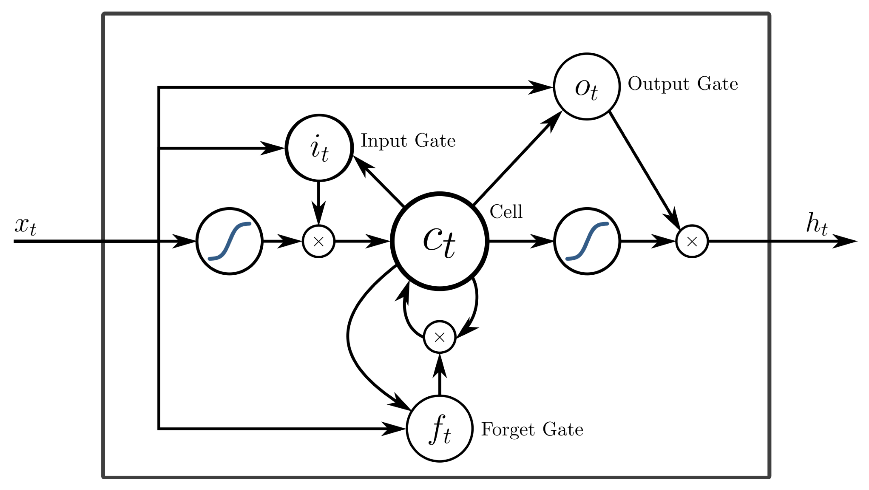
Although, this model maintains a memory of previous states, in practice it suffers from the vanishing gradient problem, thus becoming impractical for long-term dependencies [27]. A special type of RNN called Long Short Term Memory (LSTM) was published in 1997, which overcomes this issue [28]. LSTM cells follow a more sophisticated mechanism with the introduction of a complex cell that utilises “forget” gates to selectively choose what to forget. An illustration of the LSTM is given in Figure 2.
The state of an LSTM memory unit adopts the following mathematical formulation:
i t = σ ( W x i + W h i h t 1 + W c i c t 1 + b i ) f t = σ ( W x f x t + W h f h t 1 + W c f c t 1 + b f ) c t = f t c t 1 + i t t a n h ( W x c x t + W h c h t 1 + b c ) o t = σ ( W x o x t + W h o h t 1 + W c o c t + b o ) h t = o t t a n h ( c t )
To clarify, the subscripts correspond to the initials of what each matrix represents (i.e., W h f is the hidden forget weight matrix). Additionally, f, i, o and c correspond to the forget, input, output and cell gate vectors. With these in mind, an LSTM network would resemble the initial RNN architecture provided above but with LSTM cells instead.
However, due to its architecture an LSTM network can only perform forward passes on sequential data, which ultimately means that the data dependencies are only modelled uni-directionally. An intuitive way to overcome this limitation is to use an exact replica of the LSTM network but in reverse. Thus, combining these two together, a Bidirectional LSTM (BiLSTM) is created which can be used to model dependencies bidirectionally.

3.2. Embeddings

Embeddings provide an efficient mechanism for encoding the semantic and temporal context information. They were proven very effective in practical neural network applications for encoding complex data structures to information-rich continuous vectors in latent space. Examples include mappings from word to vectors [20,21,29], document to vectors [30], graphs to vectors [31], etc. Especially word vectors have become the norm in neural networks for Natural Language Processing (NLP). We address two main types of embeddings: context-free and contextual. Context-free embeddings are static and do not capture any context about the word. Conversely, a contextual embedding encapsulates information about the surrounding context of the word, hence assigning embedding vectors v i for each of the i contexts in the embedding space.

3.3. Conditional Random Fields

Conditional Random Fields (CRFs) is a discriminative model mostly used for labelling and separating sequential data [7]. The underlying concept of CRFs attempts to model a conditional probability distribution over a label sequence given an already observed sequence. The use of Conditional Random Fields (CRFs) in this work is inspired by state-of-the-art results of Neural CRFs [32] particularly combined with BiLSTMS in fundamental sequence labelling NLP tasks such as NER and POS tagging [6,33]. Neural CRFs implement neural networks to extract high-level features for use as inputs to CRFs for labelling. CRFs’ architecture models the conditional distribution P(x|y) over a label sequence, given an already observed sequence, rather than the joint distribution P(x,y), thus outperforming traditional machine learning models, such as Hidden/Maximum Entropy Markov Models (HMMs, MEMMs) [7], in sequential labelling.

3.4. Auxiliary Features (POS, IC, WS)

Although relying solely on word embeddings for prediction can deliver acceptable performance, we propose three additional features to enrich the learning significance of the semantic and syntactic abstraction of word embeddings: POS tags, Information Content (IC) and WordShape (WS).
MacDonald et al. [15] showed that specific POS n-gram sequences can be correlated with sensitive information. This provided an incentive to use POS tags as auxiliary features in this work. We extract the POS tags of the sequences using SpaCy’s v2.1 (https://github.com/explosion/spaCy) POS tagger, preferred for its speed, industrial strength and convenience.
Information Content (IC) offers a quantitative metric for general purpose sensitivity [19]. IC estimates the information carried by a specific token t in a given context, relying on the information-theoretic assumption that rare terms typically convey more information than general terms (e.g., “surgeon” vs. “doctor”). Thus, we expect that incorporating IC in our model can better classify sensitive tokens of particular classes. An example is labelling passwords: due to their random nature, the embeding of a password will most often result in the Out-Of-Vocabulary (OOV) embedding. Hence, apart from the surrounding context, there is nothing differentiating it from other OOV tokens. With this in mind, introducing IC features can be advantageous. As this, however, directly depends on the size and content of the corpus used to calculate the information content, a massive general corpus is required for general purpose estimations. To extract the IC of tokens we used the Bing search engine API (https://azure.microsoft.com/en-gb/services/cognitive-services/bing-web-search-api/). Notably, Google could be more accurate, since it maintains the largest and most updated page index to date. Yet, it was not possible to use Google’s search API for this project due to its API restrictions on repetitive use. As suggested by Sanchez et al. [19] only nouns are queued for the IC extraction as the rest of the part-of-speech types have a dynamic meaning that effectively makes search engine queries unreliable for IC calculation. These tokens are assigned an IC value of 0 by default.
Lastly, a morphological word feature, WordShape, was introduced in our experiments. We use the term WordShape as the textual representation of a word’s morphology, which is implemented through transforming words into character sequence templates. This can contribute to learning the sensitivity correlations with structured data such as credit-card numbers, national insurance numbers, and phone numbers. To generate the WordShape features, SpaCy’s v2.1 parser was used (https://spacy.io/usage/linguistic-features).

4. Dataset Creation

Public annotated datasets for token sensitivity labelling are rare. Even where such data can be collected, the subjects’ privacy is at risk through deanonymisation [34]. We therefore generate synthetic data for training purposes. Training deep learning models on synthetic data often comes with generalisability challenges due to overfitting, although recently, several scholars successfully trained such models on synthetic data in real-world settings [35]. In this paper, we developed a methodology (Section 4.2) to generate a large-enough synthetic annotated dataset, combining real-world conversational data with random sensitive information. At the highest level, two data generation approaches are used: (1) One featuring sensitivity classes that are redacted by default and (2) one with sensitivity classes that are not redacted by default. For the former, consider the data generation process for the “Online contact information” sensitivity class. For example, we choose “email” for the topic. We populate a list of conversational patterns relevant to that topic, (‘my email …’, ‘You can contact me at’, …) and use that list to search in Reddit threads using Google’s BigQuery. Then, we generate a synthetic concrete value for the sensitive part (i.e., the email address), combine it with the conversational pattern used for the query and inject it into the results as part of the conversation (comments chain). Because Google BigQuery redacts sensitive terms, we cannot ascertain their original position. Hence, the modified sentence arrays are injected at a random index. In the latter case (sensitivity classes not redacted by default) we follow a slightly different approach. Again, we use the related conversational pattern to search in Reddit threads, but this time the sensitive part is already included in the comments after the pattern. Therefore, we generate concrete values beforehand and include them in the filtering process. For instance, the “Religion” topic has a pattern “I believe in” and concrete values “Christianity”, “Buddhism”, etc., which are used as part of the query. Then we annotate the position of the sensitive concrete value and expand it until the next verb or noun is found in the sentence. Lastly, we annotate the conversational pattern “I believe in” along with the next noun. This is not a fail-proof methodology but it generated an acceptable format of the dataset that is tested in our experiments. Our synthetic datasets are derived from real conversational data from Reddit. Where used, manual annotations are part of the training process, in the same way as, for instance, human annotation in object recognition. With this approach, we increase the size of the dataset with much lower effort than that for gathering more real-world data, and we also mitigate sensitivity class imbalance [36,37,38]. We then test our proposed dataset on real unseen data.

4.1. Sensitivity Classes

To increase the semantic significance of our sensitivity classification we used 13 distinct sensitivity classes, based on the categories specified in W3C’s Platform for Privacy Preferences (P3P) [4] presented in Table 1. Note that the P3P specification originally defined 17 categories but we intentionally omitted 4 as they were very open-scoped; These are Navigation and Click-stream Data, Interactive Data, Content and Other. This made it easier to automate the aggregation of data for unambiguously defined sensitivity classes for dataset creation. It also allowed to examine model performance for each sensitivity class individually, and potentially extract more relevant insights. The choice to use the W3C P3P classes was made to (i) leverage existing legal and social expertise that informed the development of the platform, and (ii) support the openness and extensibility of our methods by allowing third-party user applications to be built on top of our work. Since P3P works with other standardised languages, such as APPEL (a P3P Preference Exchange Language), a third party automated process can use this language to trigger an action on leakage of annotated sensitive data.

4.2. Data Generation Process

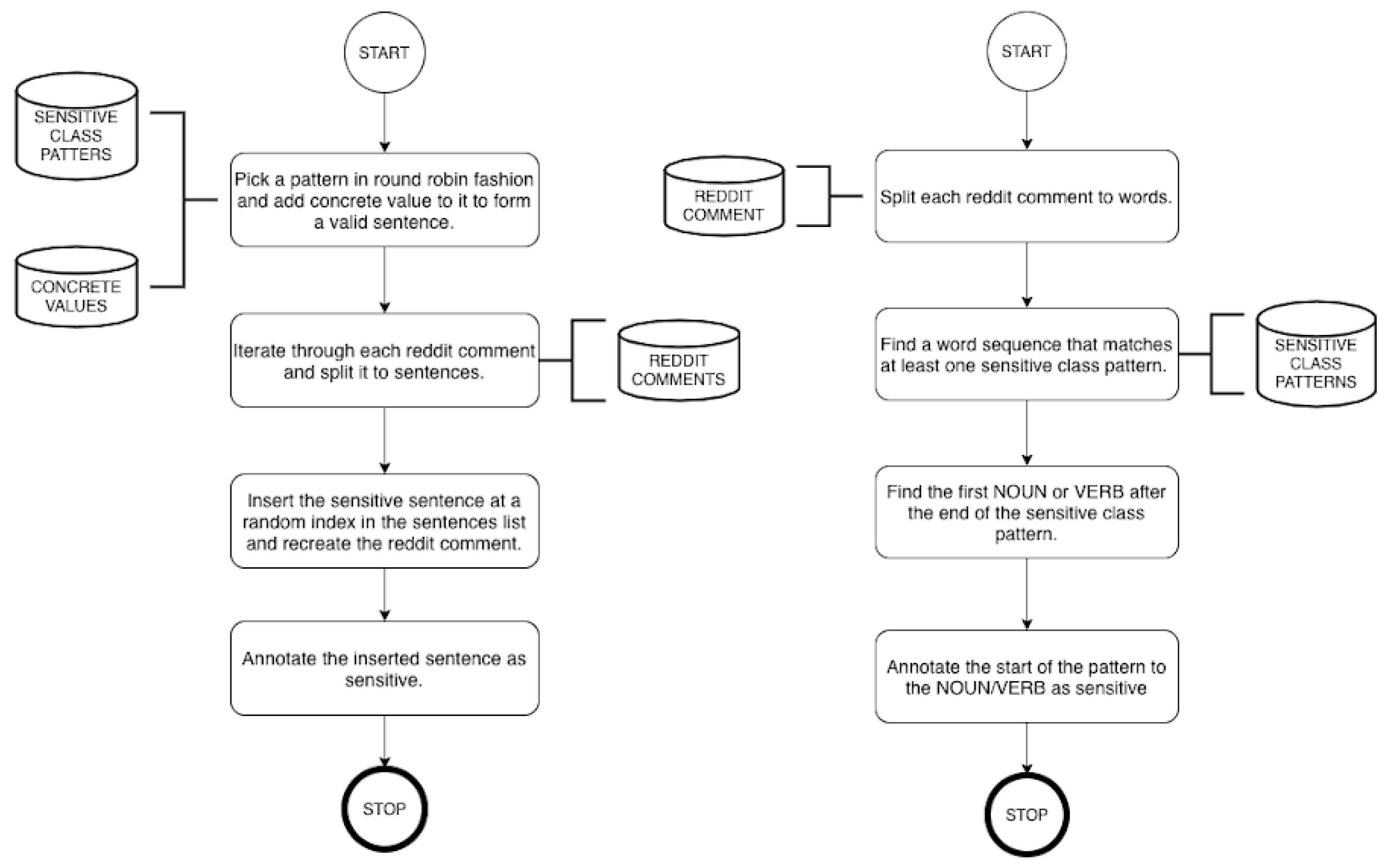
For our synthetic data generation, we extracted real-world text data from a main discussion theme and then injected sensitive data at random positions. For dataset creation purposes sensitivity classes are further divided into relevant topics, thus achieving higher granularity: for instance, the Financial Information sensitivity class would include topics like Payment History, Credit Card Numbers, Account Balance, etc. The process was repeated per topic in each sensitivity class. Because the source used for the real-world data redacts sensitive information by design, the injected text was automatically annotated as sensitive and the rest of the corpus as non-sensitive. To cover still for sensitivity classes that leak secondary private information (e.g., Preference), we developed an alternative algorithm for annotating such, not so obvious, sensitive data. A very high level flow chart of both algorithms is shown in Figure 3.
Note that the algorithms require three distinct datasets: (i) the sensitive text patterns of the topic (also used to query the data in the first place); (ii) the concrete values and; (iii) the conversational data associated with the topic. To aggregate real conversational data from the web, we utilised the publicly available Reddit comments dataset as given by Google’s BigQuery (https://bigquery.cloud.google.com/dataset/fh-bigquery:reddit_comments). The rich querying capabilities of BigQuery allowed convenient filtering for specific topics by relevant keywords.
Figure 3 (left), outlines the algorithm for augmenting our dataset with artificially created sentences that include at least one sensitive term. A sensitive term is encoded as a unique token, and then replaced with a concrete value. Concrete values are the actual mock values that make the sentence sensitive, for example, passwords, email, address These were randomly generated using Mockaroo (https://mockaroo.com/), a generation engine for realistic data.Then, the Reddit comments are split into sentences and the newly created sensitive sentence is injected at a random index within the sentence array. That sentence is annotated as sensitive and the remaining sequence as non-sensitive. The algorithm in Figure 3 (right) annotates sensitive information already present in Reddit comments. We selectively built a collection of phrases that correspond to a topic in a sensitivity class and then used these to query the Reddit comments. The phrases are then matched per comment, and all tokens from the matching phrase until the next verb or noun, are annotated as sensitive.
After data generation, we built an annotated dataset of multiple sensitivity classes. Table 1 shows the number of annotated tokens per sensitivity class in the dataset. The classes are notably imbalanced because an upper bound constraint on how many records can be generated per topic was introduced. While this constraint was imposed to avoid overfitting the model to one specific topic, the observed imbalance is realistic as it is often seen in real-world datasets [39]. Overall, 12% of the total tokens in the dataset are annotated as sensitive, with the remaining 88% labelled as non-sensitive.

5. Experimental Design

Our experiments attempt to answer three questions: (i) Which of our BiLSTM + CRF model architectures and word embeddings combination is better suited for the task; (ii) whether character embeddings contribute to increased accuracy on the model; and (iii) whether IC, POS tags and WordShape features increase model performance. For that purpose, 11 distinct BiLSTM + CRF model variations were derived for experimentation, as shown in Table 2. In addition, five simpler models were selected for bench marking against the main BiLSTM-CRF variants.
We chose the hyperparameters of the models based on empirical results [40] and preliminary experiments. The input sequences were trimmed to 205 timesteps (maximum sequence length in the dataset) and 128 units of BiLSTM cells were used, followed by a dropout layer of 40%. For experiments with character embeddings, a character input sequence of 32 length was used in a 1D convolutional layer with a kernel of size 3, followed by a dropout layer of 50% and a Global Max Pooling layer. Training was performed in batches of 128 for 100 epochs but an early stopping callback was employed to interrupt training if validation loss was not improved for 5 consecutive epochs.
The test subset consists of 10% of the dataset and was entirely left out for use as a completely unbiased evaluation dataset. The remaining 90% was further split to 80% training (used to fit the classifier weights), and 20% validation data for tuning the hyperparameters. For preprocessing, the text was converted to lowercase, all contractions were reversed and punctuation removed. Unlike conventional preprocessing pipelines, where a stopword removal stage is involved, we decided to keep the stopwords, as they are part of our automated annotation process when creating the dataset.
EXPERIMENT A:Model design and word embeddings: Interestingly, there is a wide range of BiLSTM applications in NLP often featuring state-of-the-art results [41,42,43]. Similarly, the integration of BiLSTM with a CRF layer is also rapidly gaining research attention and has delivered promising results in NLP tasks [6,33,44]. For the above reason, Experiment A focuses on reviewing the performance effect of word embeddings on BiLSTM + CRF models (see EXP. A5–A7 in Table 2). Four alternative variants (EXP. A1–A4) were also used, to offer a basis for comparison.
Even though existing literature has demonstrated the advantages of using contextualised word embeddings in numerous occasions [45,46,47], we perform this experiment to support this hypothesis for this problem setting as well. Of the many available word embedding extraction techniques [48] we shortlisted 3 methods for the evaluation, as a sufficient minimum to cover for all pre-training and contextualisation possibilities. The first uses initially random vectors to derive embeddings in the training process, and is here referred to as Randomised Word Embedding (RWE). The vocabulary of the RWE embeddings was built on the training split of our dataset. RWE is later used as a baseline for comparing with pre-trained word embeddings. The remaining two choices were pre-trained word embeddings, namely GLoVe and BERT [5,21] to cover context-free and contextualised embeddings, respectively. GLoVe is a popular context-free word embeddings model and BERT comes from Google’s BERT, a language model that achieved state-of-the-art performance in many standard NLP tasks. In the case of BERT, the output of the last encoder layer was used as embeddings.
EXPERIMENT B:Character embeddings: Character-level embeddings were successfully combined with word embeddings to improve performance before [49,50]. As the integration of character embeddings allows for learning language-agnostic morphological features, we attempt to quantify the resulting performance improvement, if any.
It has been shown that LSTM and Convolutional Neural Network (CNN) character embeddings exhibit similar performance improvements when combined with BiLSTM models, with a slight advantage for CNN [51]. We implement character embeddings through an additional extension model based on a one-dimensional convolution layer. The output of the extension model is concatenated with the input of the best-performing embedding types.
EXPERIMENT C:Auxiliary features experiment:Section 3.4 provides a detailed account of the three auxiliary features (POS, IC, WS) used to enhance model performance, and also articulated sources and selection strategies. In the experimental setting, we introduce 7 feature variations on top of the best performing BiLSTM + CRF model architecture. The aim is to practically evaluate the contribution of these features (and their combination) on performance. The variations are illustrated in Table 2 (bottom).

6. Results

Micro-averaged Precision, Recall and F1 metrics have been used for performance evaluation as they are widely used in similar sequence labelling tasks [52,53,54] and perform better on imbalanced datasets [55]. Table 2 summarises the results for the entire set of experiments carried out, separated in three sections, with the corresponding models and their performance.
EXPERIMENT A:Model design and word embeddings: As a baseline, a CRF model with casing and word morphology features was used. Table 2 shows that all of our proposed models outperform the baseline CRF. Of these, predictably, RWE performs the poorest. GLoVe embeddings deliver a substantial improvement, with BERT embeddings giving the best results across all three metrics, most likely due to its contextualised nature. On aggregate, results indicate that adding a CRF layer improves the performance of all models slightly. In summary, although the increase of the F1 metric is very marginal, there is a consistent improvement throughout all variants in experiment A when introducing a CRF layer. We observe that BiLSTM BERT + CRF is the best performing CRF-enriched model in regards to model architecture and embeddings.
EXPERIMENT B:Character embeddings: Despite our expectation for the contrary, results revealed that character embeddings cause performance deterioration. Reasons for this may be: (a) that the supplementary trainable parameters increased the model’s complexity and learning the underlying correlations between the data points became more challenging, and (b) that the CNN and pooling architecture is perhaps by design unsuitable for this problem setting. The remaining experiments were conducted without CNN character embeddings.
EXPERIMENT C:Auxiliary features experiment: For the third part of the experiment we used POS tags, IC and WordShape as auxiliary features for the classification. Overall, it is observed that the combination of two or more auxiliary features offers a slight performance advantage against single feature models. Yet, the performance metrics when using those features are not dissimilar from the initial BiLSTM + CRF model with BERT embeddings, except when using WordShape features exclusively. Thus, based on the Recall and F1 metrics, we identify WordShape as a better suited auxiliary feature that can be used with BiLSTM + CRF model. Accordingly, we chose to incorporate WordShape features for further evaluation experiments.

7. Evaluation

Based on the experimental results presented in Section 6 we evaluate BiLSTMBERT+WS + CRF against temporal and semantic context sensitivity labelling.
For temporal context sensitivity labelling, the final model is evaluated on a dataset that was manually built and annotated. Manual annotation is time-consuming and thus the dataset is small compared to the synthetic one. It consists of 60 text sequences, specifically written in a way that token sensitivity is directly dependent on temporal context.
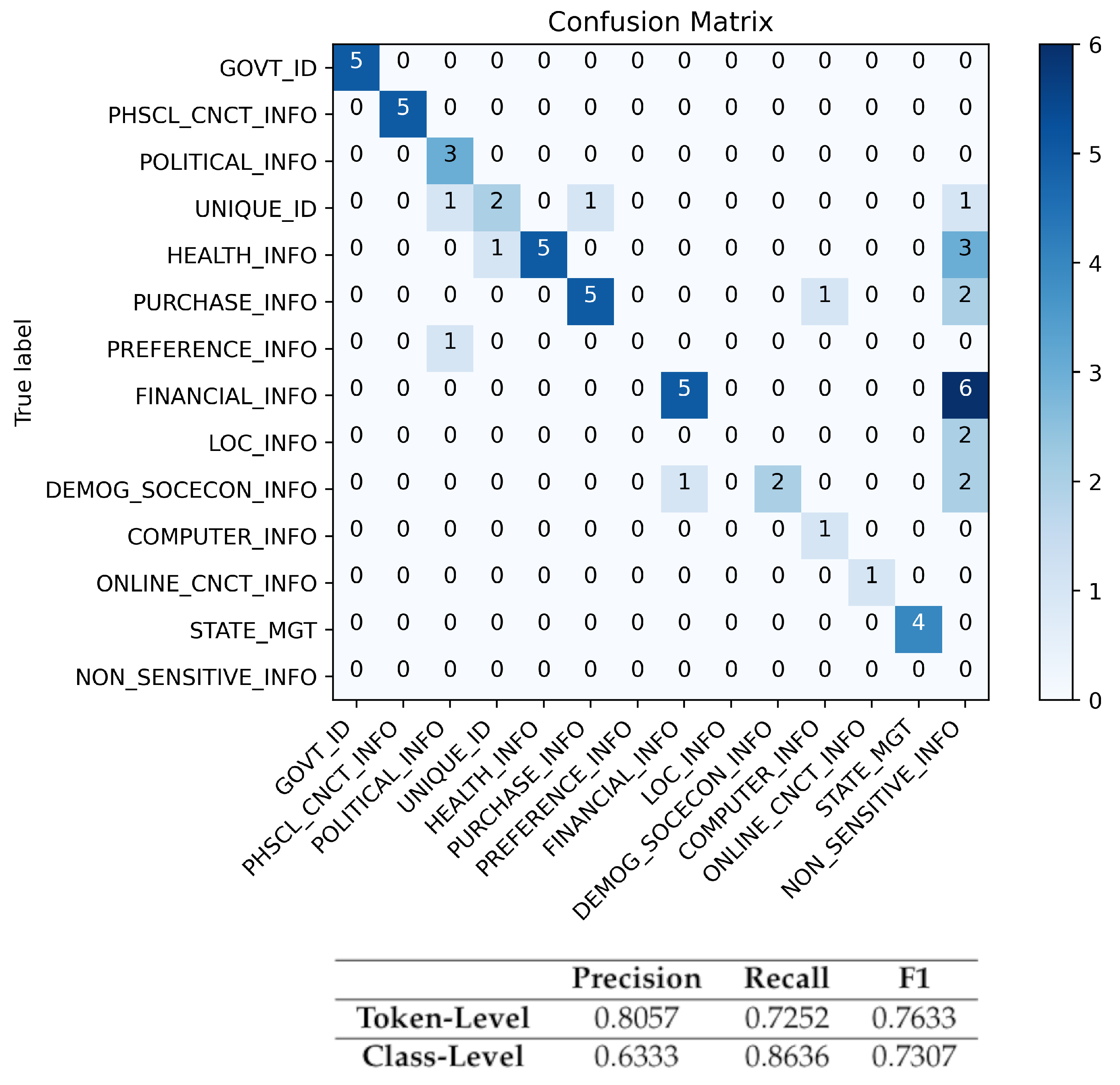
Due to manual annotation, there were cases where stopwords were annotated as sensitive tokens but not picked up by the model, or vice versa, causing a drop in the evaluation metrics. A confusion matrix (Figure 4) on class-level (rather than token level) granularity offers a better evaluation that is invariant to annotation discrepancies. In effect this demonstrates whether the model managed to identify the sensitivity class of the text. Figure 4 illustrates that the majority of sensitivity types are classified correctly. Most of the incorrect classifications are confused with the NON_SENSITIVE class. Note that the hardest classes to classify are the DEMOG_SOCECON_INFO and POLITICAL_INFO. Additionally, it is important to highlight that the 76.33% and 73.07% F1 score in token-level and class-level experiments, respectively (Figure 4), support our hypothesis that a BiLSTM model can be used for temporal context sensitivity annotation.
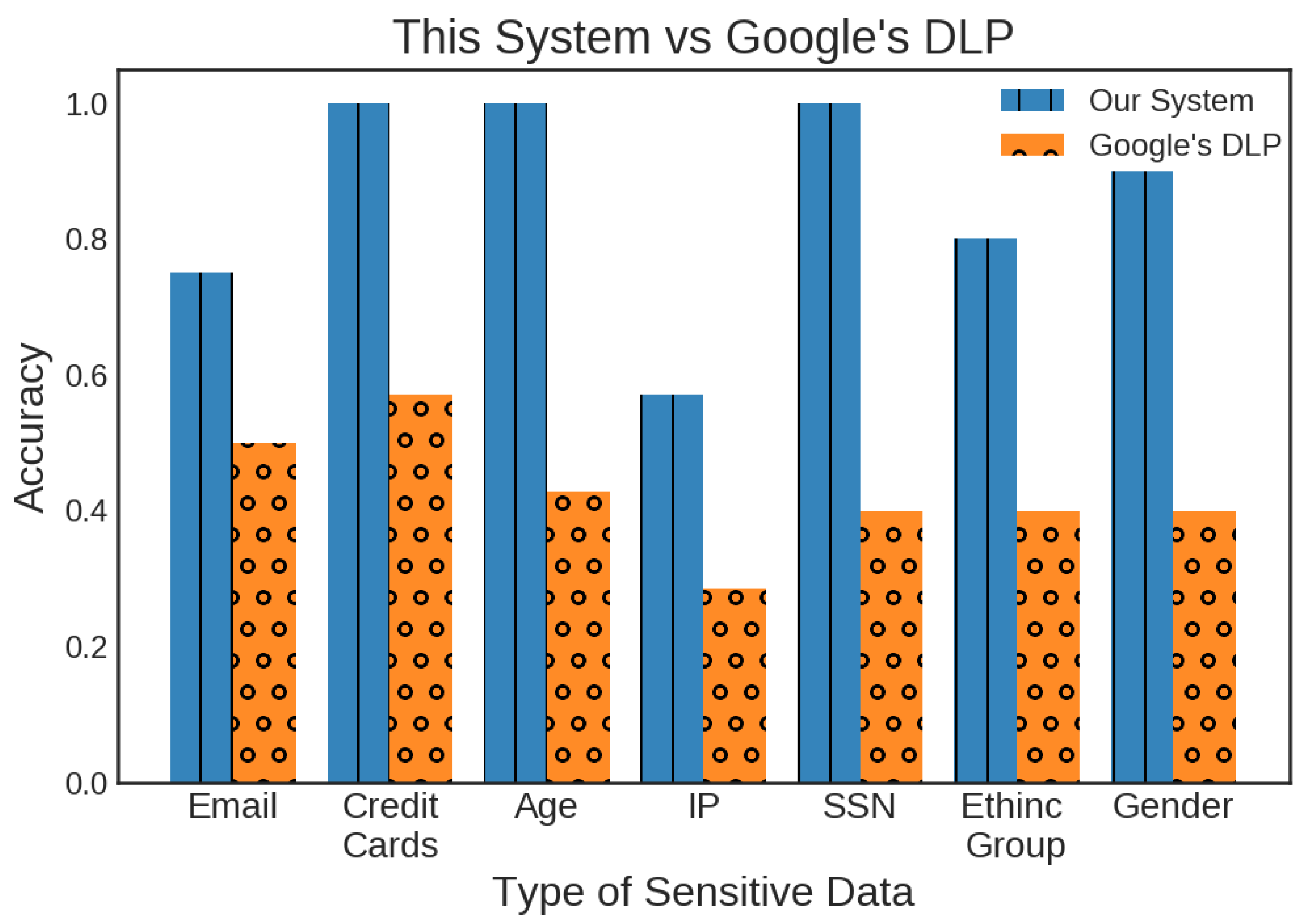
For our Semantic Context Evaluation, we performed a comparative evaluation against Google’s DLP system (https://cloud.google.com/dlp/), which provides industrial-strength sensitive data annotation for over 80 sensitive data types. Google DLP is chosen for its industrial strength and was seen as a suitable benchmark for semantic evaluation since it also uses an automated methodology. To perform an as accurate as possible comparison, we test the performance of the two systems (our model and DLP) solely on sensitive data types, which are common between the two. Google DLP is provided as a platform with standard functionality, allowing solely for user intervention in (i) selecting InfoTypes (equivalent to topics of our Sensitivity Classes) and; (ii) creating templates to support a more structured data detection approach. To that end, another dataset was created manually, containing text sequences that include sensitive tokens affected by semantic context (as an example of a sample in this dataset, consider the sentences “I am a male” and “I am a man”, they both reveal the same gender information but the wording is different). In the absence of sizeable overlap between the two systems on sensitivity topics, we select only those commonly appearing in both. These are: Email, Credit Cards, Age, IP, SSN, Ethnic Group and Gender.
Results of our comparison are provided in Figure 5. For all sensitive data types, our system outperforms Google’s DLP service. Particularly it was observed that, when noise that can affect the syntactic but not the semantic meaning of sensitive data was added, Google’s DLP fails to annotate the sensitive tokens. On the contrary, our system exhibits resilience against such noise with a relative accuracy advantage over the Google DLP of 42.65%.

8. Discussion

Sensitive information labelling is a prominent problem when designing privacy-aware decision systems. Automated sensitivity labelling is especially relevant when considering users as custodians of their own personal data. With this in mind, we developed our model to enhance sensitivity annotation by first offering a taxonomy of four context classes (semantic, agent, temporal and self), and then using these to implement context-aware labelling.
Our model does not come without limitations, and future work should: involve the full set of context classes; extend the auxiliary features experiments to evaluate tweaked models such as plain BiLSTM (without CRF); incorporate additional word, sentence and character embeddings; and perform testing and validation on more extensive datasets. Yet, the work presented in this paper can essentially serve as a framework for building similar models within alternative well-defined problem domains.
The impact of our work is manifold, although we acknowledge potential risks that typically come with advancements in understanding and extracting sensitive information. While our models contribute to more accurate context-aware sensitivity labelling, our choice to adopt P3P sensitivity classes also supports openness and extensibility to third party applications, offering a platform for others to further develop suitable methods. It furthermore demonstrates promising results from using deep learning techniques in text sensitivity annotation, an area that is sparsely addressed in the literature. We believe that further expanding our approach will offer a more concrete future direction for privacy-preserving information exchange.

Author Contributions

This paper was accomplished based on the collaborative work of the authors. A.P. performed the experiments and analysed the data. Experiment interpretation and paper authorship were jointly performed by A.P. and G.S. All authors have read and agreed to the published version of the manuscript.

Funding

This research received no external funding.

Conflicts of Interest

The authors declare no conflict of interest.

Abbreviations

The following abbreviations are used in this manuscript:
BERTBidirectional Encoder Representations from Transformers
BiLSTMBidirectional Lond-Short Term Memory
CNNConvolutional Neural Network
CRFConditional Random Field
CWIComplex Word Identification
DLPData Loss Prevention
ICInformation Context
LSTMLong Short Term Memory
RNNRecurrent Neural Network
NERNamed Entity Recognition
OOVOut-of-Vocabulary
POSPart of Speech
SVMSupport Vector Machine
WSWordShape

References

  1. Acquisti, A.; Adjerid, I.; Balebako, R.; Brandimarte, L.; Cranor, L.F.; Komanduri, S.; Leon, P.G.; Sadeh, N.; Schaub, F.; Sleeper, M.; et al. Nudges for privacy and security: Understanding and assisting users’ choices online. ACM Comput. Surv. (CSUR) 2017, 50, 1–41. [Google Scholar] [CrossRef] [Green Version]
  2. Acquisti, A.; Grossklags, J. Privacy and rationality in individual decision making. IEEE Secur. Priv. 2005, 3, 26–33. [Google Scholar] [CrossRef]
  3. Wang, Y.; Norcie, G.; Komanduri, S.; Acquisti, A.; Leon, P.G.; Cranor, L.F. I regretted the minute I pressed share: A qualitative study of regrets on Facebook. In Proceedings of the Seventh Symposium on Usable Privacy and Security, Pittsburgh, PA, USA, 20–22 July 2011; ACM: New York, NY, USA, 2011; p. 10. [Google Scholar]
  4. Cranor, L.; Dobbs, B.; Egelman, S.; Hogben, G.; Humphrey, J.; Langheinrich, M.; Marchiori, M.; Presler-Marshall, M.; Reagle, J.M.; Schunter, M.; et al. The Platform for Privacy Preferences 1.1 (P3P1.1) Specification; Note NOTE-P3P11-20061113; World Wide Web Consortium: Cambridge, MA, USA, 2006. [Google Scholar]
  5. Devlin, J.; Chang, M.W.; Lee, K.; Toutanova, K. Bert: Pre-training of deep bidirectional transformers for language understanding. arXiv 2018, arXiv:1810.04805. [Google Scholar]
  6. Ma, X.; Hovy, E. End-to-end sequence labeling via bi-directional lstm-cnns-crf. arXiv 2016, arXiv:1603.01354. [Google Scholar]
  7. Lafferty, J.; McCallum, A.; Pereira, F.C. Conditional Random Fields: Probabilistic Models for Segmenting and Labeling Sequence Data. Available online: https://repository.upenn.edu/cis_papers/159/ (accessed on 13 June 2020).
  8. Ong, Y.J.; Qiao, M.; Routray, R.; Raphael, R. Context-Aware Data Loss Prevention for Cloud Storage Services. In Proceedings of the 2017 IEEE 10th International Conference on Cloud Computing (CLOUD), Honolulu, CA, USA, 25–30 June 2017; pp. 399–406. [Google Scholar] [CrossRef]
  9. Alzhrani, K.; Rudd, E.M.; Boult, T.E.; Chow, C.E. Automated Big Text Security Classification. In Proceedings of the 2016 IEEE Conference on Intelligence and Security Informatics (ISI), Tucson, AZ, USA, 28–30 September 2016. [Google Scholar]
  10. Hart, M.; Manadhata, P.; Johnson, R. Text classification for data loss prevention. In Proceedings of the 11th International Conference on Privacy Enhancing Technologies, Waterloo, ON, Canada, 24 July 2011; Springer: Berlin/Heidelberg, Germany, 2011. [Google Scholar]
  11. Gomez-Hidalgo, J.M.; Martin-Abreu, J.M.; Nieves, J.; Santos, I.; Brezo, F.; Bringas, P.G. Data leak prevention through named entity recognition. In Proceedings of the 2010 IEEE Second International Conference on Social Computing, Minneapolis, MN, USA, 20–22 August 2010; pp. 1129–1134. [Google Scholar]
  12. Alneyadi, S.; Sithirasenan, E.; Muthukkumarasamy, V. Word N-gram based classification for data leakage prevention. In Proceedings of the 2013 12th IEEE International Conference on Trust, Security and Privacy in Computing and Communications, Melbourne, Australia, 16–18 July 2013; pp. 578–585. [Google Scholar]
  13. McDonald, G.; Macdonald, C.; Ounis, I.; Gollins, T. Towards a classifier for digital sensitivity review. In European Conference on Information Retrieval; Springer: Berlin/Heidelberg, Germany, 2014; pp. 500–506. [Google Scholar]
  14. McDonald, G.; Macdonald, C.; Ounis, I. Enhancing sensitivity classification with semantic features using word embeddings. In European Conference on Information Retrieval; Springer: Berlin/Heidelberg, Germany, 2017; pp. 450–463. [Google Scholar]
  15. McDonald, G.; Macdonald, C.; Ounis, I. Using part-of-speech n-grams for sensitive-text classification. In Proceedings of the 2015 International Conference on The Theory of Information Retrieval, Northampton, MA, USA, 27–30 September 2015; ACM: New York, NY, USA, 2015; pp. 381–384. [Google Scholar]
  16. Caliskan Islam, A.; Walsh, J.; Greenstadt, R. Privacy detective: Detecting private information and collective privacy behavior in a large social network. In Proceedings of the 13th Workshop on Privacy in the Electronic Society, Scottsdale, AZ, USA, 3 November 2014; ACM: New York, NY, USA, 2014; pp. 35–46. [Google Scholar]
  17. Jiang, K.; Feng, S.; Song, Q.; Calix, R.A.; Gupta, M.; Bernard, G.R. Identifying tweets of personal health experience through word embedding and LSTM neural network. BMC Bioinform. 2018, 19, 210. [Google Scholar] [CrossRef] [PubMed]
  18. Sweeney, L. Replacing personally-identifying information in medical records, the Scrub system. In Proceedings of the AMIA Annual Fall Symposium 1996, Washington, DC, USA, 30 October 1996; American Medical Informatics Association: Bethesda, MD, USA, 1996; p. 333. [Google Scholar]
  19. Sánchez, D.; Batet, M.; Viejo, A. Detecting sensitive information from textual documents: An information- theoretic approach. In International Conference on Modeling Decisions for Artificial Intelligence; Springer: Berlin/Heidelberg, Germany, 2012; pp. 173–184. [Google Scholar]
  20. Mikolov, T.; Sutskever, I.; Chen, K.; Corrado, G.S.; Dean, J. Distributed representations of words and phrases and their compositionality. In Advances in Neural Information Processing Systems; ACM: New York, NY, USA, 2013; pp. 3111–3119. [Google Scholar]
  21. Pennington, J.; Socher, R.; Manning, C.D. GloVe: Global Vectors for Word Representation. In Proceedings of the 2014 Conference on Empirical Methods in Natural Language Processing (EMNLP), Doha, Qatar, 25–29 October 2014; pp. 1532–1543. [Google Scholar]
  22. Ali, F.; El-Sappagh, S.; Kwak, D. Fuzzy Ontology and LSTM-Based Text Mining: A Transportation Network Monitoring System for Assisting Travel. Sensors 2019, 19, 234. [Google Scholar] [CrossRef] [PubMed] [Green Version]
  23. Ali, F.; El-Sappagh, S.; Islam, S.R.; Ali, A.; Attique, M.; Imran, M.; Kwak, K.S. An intelligent healthcare monitoring framework using wearable sensors and social networking data. Future Gener. Comput. Syst. 2021, 114, 23–43. [Google Scholar] [CrossRef]
  24. Ayvaz, E.; Kaplan, K.; Kuncan, M. An Integrated LSTM Neural Networks Approach to Sustainable Balanced Scorecard-Based Early Warning System. IEEE Access 2020, 8, 37958–37966. [Google Scholar] [CrossRef]
  25. Bengio, Y.; Simard, P.; Frasconi, P. Learning long-term dependencies with gradient descent is difficult. IEEE Trans. Neural Netw. 1994, 5, 157–166. [Google Scholar] [CrossRef] [PubMed]
  26. Salehinejad, H.; Sankar, S.; Barfett, J.; Colak, E.; Valaee, S. Recent advances in recurrent neural networks. arXiv 2017, arXiv:1801.01078. [Google Scholar]
  27. Hochreiter, S. The vanishing gradient problem during learning recurrent neural nets and problem solutions. Int. J. Uncertain. Fuzziness Knowl. Based Syst. 1998, 6, 107–116. [Google Scholar] [CrossRef] [Green Version]
  28. Hochreiter, S.; Schmidhuber, J. Long short-term memory. Neural Comput. 1997, 9, 1735–1780. [Google Scholar] [CrossRef] [PubMed]
  29. Shi, B.; Fu, Z.; Bing, L.; Lam, W. Learning Domain-Sensitive and Sentiment-Aware Word Embeddings. arXiv 2018, arXiv:1805.03801. [Google Scholar]
  30. Le, Q.; Mikolov, T. Distributed representations of sentences and documents. In Proceedings of the International Conference on Machine Learning, Beijing, China, 21–26 June 2014; pp. 1188–1196. [Google Scholar]
  31. Narayanan, A.; Chandramohan, M.; Venkatesan, R.; Chen, L.; Liu, Y.; Jaiswal, S. graph2vec: Learning Distributed Representations of Graphs. arXiv 2017, arXiv:1707.05005. [Google Scholar]
  32. Artieres, T. Neural conditional random fields. In Proceedings of the Thirteenth International Conference on Artificial Intelligence and Statistics, Sardinia, Italy, 13–15 May 2010; pp. 177–184. [Google Scholar]
  33. Lample, G.; Ballesteros, M.; Subramanian, S.; Kawakami, K.; Dyer, C. Neural architectures for named entity recognition. arXiv 2016, arXiv:1603.01360. [Google Scholar]
  34. Narayanan, A.; Shmatikov, V. How to break anonymity of the netflix prize dataset. arXiv 2006, arXiv:cs/0610105. [Google Scholar]
  35. Emam, K.; Mosquera, L.; Hoptroff, R. Practical Synthetic Data Generation: Balancing Privacy and the Broad Availability of Data; O’Reilly Media, Incorporated: Sebastopol, CA, USA, 2020. [Google Scholar]
  36. Hu, G.; Peng, X.; Yang, Y.; Hospedales, T.M.; Verbeek, J. Frankenstein: Learning deep face representations using small data. IEEE Trans. Image Process. 2018, 27, 293–303. [Google Scholar] [CrossRef] [Green Version]
  37. Das, A.; Gkioxari, G.; Lee, S.; Parikh, D.; Batra, D. Neural Modular Control for Embodied Question Answering. arXiv 2018, arXiv:1810.11181. [Google Scholar]
  38. Patki, N.; Wedge, R.; Veeramachaneni, K. The synthetic data vault. In Proceedings of the 2016 IEEE International Conference on Data Science and Advanced Analytics (DSAA), Montreal, QC, Canada, 17–19 October 2016; pp. 399–410. [Google Scholar]
  39. Kaur, H.; Pannu, H.S.; Malhi, A.K. A Systematic Review on Imbalanced Data Challenges in Machine Learning: Applications and Solutions. ACM Comput. Surv. 2019, 52. [Google Scholar] [CrossRef] [Green Version]
  40. Cheng, G.; Peddinti, V.; Povey, D.; Manohar, V.; Khudanpur, S.; Yan, Y. An Exploration of Dropout with LSTMs. In Proceedings of the Interspeech, Stockholm, Sweden, 20–24 August 2017. [Google Scholar]
  41. Wang, A.; Singh, A.; Michael, J.; Hill, F.; Levy, O.; Bowman, S.R. Glue: A multi-task benchmark and analysis platform for natural language understanding. arXiv 2018, arXiv:1804.07461. [Google Scholar]
  42. Talman, A.; Yli-Jyrä, A.; Tiedemann, J. Natural Language Inference with Hierarchical BiLSTM Max Pooling Architecture. arXiv 2018, arXiv:1808.08762. [Google Scholar]
  43. Bohnet, B.; McDonald, R.T.; Simões, G.; Andor, D.; Pitler, E.; Maynez, J. Morphosyntactic Tagging with a Meta-BiLSTM Model over Context Sensitive Token Encodings. arXiv 2018, arXiv:1805.08237. [Google Scholar]
  44. Reimers, N.; Gurevych, I. Reporting Score Distributions Makes a Difference: Performance Study of LSTM-networks for Sequence Tagging. arXiv 2017, arXiv:1707.09861. [Google Scholar]
  45. Si, Y.; Wang, J.; Xu, H.; Roberts, K. Enhancing Clinical Concept Extraction with Contextual Embedding. arXiv 2019, arXiv:1902.08691. [Google Scholar] [CrossRef] [Green Version]
  46. MacAvaney, S.; Yates, A.; Cohan, A.; Goharian, N. CEDR: Contextualized Embeddings for Document Ranking. arXiv 2019, arXiv:1904.07094. [Google Scholar]
  47. Reimers, N.; Schiller, B.; Beck, T.; Daxenberger, J.; Stab, C.; Gurevych, I. Classification and Clustering of Arguments with Contextualized Word Embeddings. In Proceedings of the 57th Annual Meeting of the Association for Computational Linguistics, Florence, Italy, 28 July–2 August 2019; Association for Computational Linguistics: Florence, Italy, 2019; pp. 567–578. [Google Scholar] [CrossRef]
  48. Gutiérrez, L.; Keith, B. A Systematic Literature Review on Word Embeddings. In International Conference on Software Process Improvement; Springer: Berlin/Heidelberg, Germany, 2018; pp. 132–141. [Google Scholar]
  49. Xin, Y.; Hart, E.; Mahajan, V.; Ruvini, J. Learning Better Internal Structure of Words for Sequence Labeling. arXiv 2018, arXiv:1810.12443. [Google Scholar]
  50. Yuan, H.; Yang, Z.; Chen, X.; Li, Y.; Liu, W. URL2Vec: URL Modeling with Character Embeddings for Fast and Accurate Phishing Website Detection. In Proceedings of the 2018 IEEE International Conference on Parallel Distributed Processing with Applications, Ubiquitous Computing Communications, Big Data Cloud Computing, Social Computing Networking, Sustainable Computing Communications (ISPA/IUCC/BDCloud/SocialCom/SustainCom), Melbourne, Australia, 11–13 December 2018; pp. 265–272. [Google Scholar] [CrossRef]
  51. Zhai, Z.; Nguyen, D.Q.; Verspoor, K. Comparing CNN and LSTM character-level embeddings in BiLSTM-CRF models for chemical and disease named entity recognition. arXiv 2018, arXiv:1808.08450. [Google Scholar]
  52. Tjong Kim Sang, E.F.; De Meulder, F. Introduction to the CoNLL-2003 Shared Task: Language-Independent Named Entity Recognition. In Proceedings of the Seventh Conference on Natural Language Learning at HLT-NAACL 2003, Edmonton, Canada, 31 May–1 June 2003; pp. 142–147. [Google Scholar]
  53. Zhu, S.; Yu, K. Encoder-decoder with focus-mechanism for sequence labelling based spoken language understanding. In Proceedings of the 2017 IEEE International Conference on Acoustics, Speech and Signal Processing (ICASSP), New Orleans, LA, USA, 5–9 March 2017; pp. 5675–5679. [Google Scholar]
  54. Pahuja, V.; Laha, A.; Mirkin, S.; Raykar, V.; Kotlerman, L.; Lev, G. Joint learning of correlated sequence labelling tasks using bidirectional recurrent neural networks. arXiv 2017, arXiv:1703.04650. [Google Scholar]
  55. Johnson, J.M.; Khoshgoftaar, T.M. Survey on deep learning with class imbalance. J. Big Data 2019, 6, 27. [Google Scholar] [CrossRef]
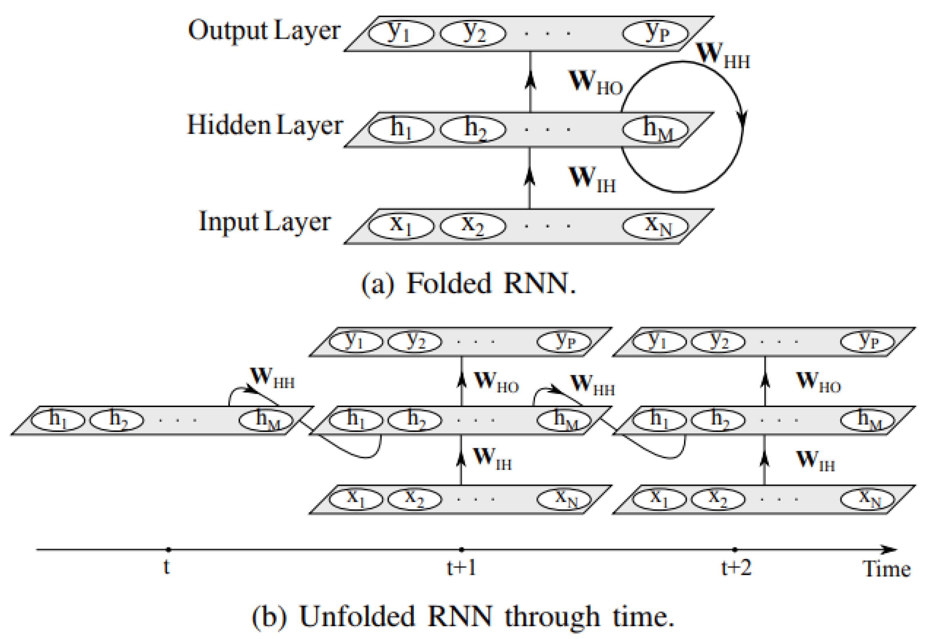
Figure 1. Simple Recurrent Neural Network (RNN) architecture. For the sake of simplicity biases are ignored. Source: [26].
Applsci 10 08924 g001
Figure 2. Long Short Term Memory (LSTM) unit. For the sake of simplicity biases are ignored.
Applsci 10 08924 g002
Figure 3. Synthetic data generation (i) when sensitive data is redacted by default (left) and (ii) when it is not (right).
Applsci 10 08924 g003
Figure 4. Confusion matrix for temporal context evaluation.
Applsci 10 08924 g004
Figure 5. Comparative evaluation between our system and Google’s Data Loss Prevention (DLP) system.
Applsci 10 08924 g005
Table 1. Sensitivity classes used for multi-class classification. (Source: P3P Standard [4]) and the count of sensitive tokens in our dataset per class.
Sensitivity ClassDescriptionLabelCount
Physical Contact InformationInformation that allows an individual to be contacted or located in the physical world—such as telephone number or address.PHSCL_CNCT_INFO14,108
Online Contact InformationInformation that allows an individual to be contacted or located on the Internet—such as email. Often, this information is independent of the specific computer used to access the network. (See the category “Computer Information”)ONLINE_CNCT_INFO30,248
Unique IdentifiersNon-financial identifiers, excluding government-issued identifiers, issued for purposes of consistently identifying or recognising the individual. These include identifiers issued by a Web site or service.UNIQUE_ID10,594
Purchase InformationInformation actively generated by the purchase of a product or service, including information about the method of payment.PURCHASE_INFO13,712
Financial InformationInformation about an individual’s finances including account status and activity information such as account balance, payment or overdraft history, and information about an individual’s purchase or use of financial instruments including credit or debit card information.FINANCIAL_INFO19,258
Computer InformationInformation about the computer system that the individual is using to access the network—such as the IP number, domain name, browser type or operating system.COMPUTER_INFO8143
Demographic and Socioeconomic DataData about an individual’s characteristics—such as gender, age, income, postal code, or geographic region.DEMOG_SOCECON_INFO26,013
State Management MechanismsMechanisms for maintaining a stateful session with a user or automatically recognising users who have visited a particular site or accessed particular content previously—such as HTTP cookies.STATE_MGT5666
Political InformationMembership in or affiliation with groups such as religious organisations, trade unions, professional associations, political parties, etc.POLITICAL_INFO21,341
Health InformationInformation about an individual’s physical or mental health, sexual orientation, use or inquiry into health care services or products, and purchase of health care services or products.HEALTH_INFO23,516
Preference DataData about an individual’s likes and dislikes—such as favorite colour or musical tastes.PREFERENCE_INFO43,048
Location DataInformation that can be used to identify an individual’s current physical location and track them as their location changes—such as GPS position data.LOC_INFO15,795
Government-issued IdentifiersIdentifiers issued by a government for purposes of consistently identifying the individual.GOVT_ID14,108
Table 2. Model variations and performance metrics of the experiments. (Top Section): Conditional Random Fields (CRF) layer and embeddings combination results. (Middle Section): Character embeddings model extension experiment results. (Bottom Section): Auxiliary features variations experiment results.
MODELEMBEDDINGSAUX. FEATURESRESULTS
BiLSTMCRFCNNRWEGLoVeBERTPOSICWSPrecisionRecallF1
EXP. A1 X 0.80680.57790.6581
2X X 0.89860.93150.9147
3X X 0.93470.95990.9471
4X X 0.94520.96890.9569
5XX X 0.91130.93370.9224
6XX X 0.94510.95580.9504
7XX X 0.95680.96930.9630
EXP B.8X X X 0.95680.95760.9572
9XXX X 0.96340.95580.9596
EXP C.10XX XX 0.95480.96850.9616
11XX X X 0.96110.96180.9614
12XX X X0.96400.97060.9673
13XX XXX 0.96390.96250.9631
14XX X XX0.96350.96290.9632
15XX XX X0.96280.96150.9622
16XX XXXX0.96110.97040.9657
Publisher’s Note: MDPI stays neutral with regard to jurisdictional claims in published maps and institutional affiliations.