Article

Fluctuations in the Homogeneity of Cell Medium Distinguish Benign from Malignant Lymphocytes in a Cellular Model of Acute T Cells Leukemia

Racah Institute of Physics, The Hebrew University, Jerusalem 9190401, Israel
*
Author to whom correspondence should be addressed.
Appl. Sci. 2020, 10(24), 8894; https://doi.org/10.3390/app10248894
Submission received: 25 October 2020 / Revised: 5 December 2020 / Accepted: 10 December 2020 / Published: 13 December 2020
(This article belongs to the Section Applied Biosciences and Bioengineering)

Abstract

:
Intracellular mechanical work facilitates multiple cell functions, such as material transport, cell motility, etc., and is indicative of the cell’s physiological condition. Still, the characterization of intracellular mechanical work and resultant dynamics remain hard to determine in intact label-free cells. For that, we imaged live T cells via bright-field microscopy and studied fluctuations in the homogeneity of their intracellular medium. Specifically, we characterized medium homogeneity and dynamics by using the information entropy of its related intensity gray levels (termed Gray Level Information Entropy (GLIE)) and spectral analysis of GLIE fluctuations, respectively. First, we provide simple examples of particle motion, to demonstrate the utility of our approach. Using this approach, we could further study and distinguish mitochondrial dysfunction and ATP depletion state in live Jurkat cells. The relation of our results to intracellular dynamics was confirmed by comparison to image correlation spectroscopy (ICS) results in the same cells. Importantly, GLIE fluctuations combined with spectral analysis enabled differentiation of malignant Jurkat cells from benign lymphocytes with 86% accuracy for single cells and 95% for populations of 10 cells each. Our approach can serve for label-free live-cell study and diagnostics of important pathophysiological conditions, such as mitochondrial dysfunction and malignancy.

1. Introduction

Cells rely on ATP consumption and mechanical work for their multiple functions, such as material transport, cell motility, etc. [1,2]. This mechanical work may dominate intracellular dynamics in comparison to thermal agitation in time scales longer than 100 ms [3,4]. Molecular motors, such as myosin, produce directed and undirected motion inside cells, as they move along the viscoelastic cytoskeleton and generate ATP-dependent forces [2,5]. Such forces, acting at multiple sites and times on the cytoskeleton, have an incoherent fraction that produces complex modes of vibration of that cytoskeleton. These vibrations can generate a complex motion of intracellular structures, e.g., vesicles or organelles that are embedded inside the cytoskeleton mesh and are typically larger than the mesh size (around 50 nm) [4]. The resultant motion is “random-walk-like” (not necessarily with white noise characteristics) [3]. This motion is the result of multiple forces that act at different times and spatial points on the cytoskeleton. Therefore, it reflects a summation of many forces that relate to the extent of mechanical activity of the cell. Thus, by monitoring intracellular dynamics, one can expose the degree of mechanical work and motion in that cell [6]. Cellular mechanical activity and intracellular dynamics relate to the cell’s physiological condition—mainly regarding energy production [4,7,8] and mode of metabolism (e.g., normal vs. malignant cell metabolism) [4,9,10]. They also relate to intracellular rheology parameters, such as elasticity and viscosity [3].
Previously, Guo et al. [4] described how mechanical work and motion are reduced after cellular ATP depletion. These parameters were higher in malignant cells, relative to benign cells. Their work utilized tracking of intracellular injected nano-particles, vesicles and proteins complexes in multiple benign and malignant cells. Indeed, intracellular particle tracking is a powerful experimental tool for evaluation of cell dynamics [9,10,11,12]. The analysis of that intracellular dynamic’s characteristics could reveal cellular pathophysiology conditions, such as malignancy, activation, or mitochondrial dysfunction and ATP depletion. Still, this method has some prominent disadvantages that prevent the application of this method for clinical use. Disadvantages include the need to apply thresholds to the original images in order to rely on a specific range of pixel intensities (while ignoring the other pixels data). Then, this process requires collecting a large number of trajectories that usually have a broad distribution of motion characteristics. The analysis in this approach is very time consuming and difficult to automate. This makes that approach more suitable for laboratory research than for clinical use. Other experimental methods to analyze intracellular dynamics, such as Optical Coherence Tomography (OCT) speckle decorrelation [13] or Diffusion NMR spectroscopy [14], require much more advanced experimental setup.
In addition to particle tracking, time-dependent fluctuations in general characteristics of the medium, such as homogeneity or information entropy, may depend on intracellular motion. By that, they could also applied for the study of intracellular dynamics [15]. Through this approach, all pixels of a cell image can be considered for analysis. In contrast, when using particles tracking, only a selection of specific pixels that characterize the contour of particles are followed. That kind of process, which relies on a small number of selected pixels, requires high resolution and low errors of localization. Monitoring changes in pixels’ homogeneity or in their Gray Level Information Entropy (GLIE) is less optically demanding because there is no need to follow the motion of the delicate contour line of particles. Instead, GLIE fluctuations monitor the general chance of all image pixels to experience changes in gray levels due to particles motion. Evaluation of cell dynamics through GLIE fluctuation analysis enabled differentiation of live from dead cells [16] and exploration of a range of cellular physiological conditions that included malignancy [8,15].
Complex intracellular dynamics often result in anomalous diffusion [12,17,18]. Brownian diffusion and multiple types of anomalous diffusion can be related by analytical models to a Power Spectral Density (PSD) description of motion that obeys the following general formula: P o w e r   ( f , ) = D f β , where f represents frequency, β relates to the power of diffusion and D represents a constant that is correlated to the diffusion coefficient (Kα) [19,20,21]. PSD (or Amplitude Spectral Density (ASD)) analysis of motion with its fitted power formula enables the determination of specific motion characteristics, including the diffusion coefficient, the power of diffusion and a break in ergodicity [19,20,21].
Here, we aim to combine the detection and characterization of intracellular motion by monitoring GLIE changes of the inspected medium with the PSD analysis of these changes and their power-fits. In that way, we wish to combine the sensitivity of GLIE changes in the detection of intracellular motion with the efficiency of PSD analysis in resolving this motion. We first study theoretically the sensitivity of our analysis of pixels GLIE through simple examples of particle motion. Next, we test experimentally, in living cells, the response of GLIE fluctuation parameters to a state of reduced intracellular dynamics due to mitochondrial dysfunction and ATP depletion. Finally, we explore the possible use of GLIE fluctuation parameters to differentiate malignant lymphocytes (Jurkat cells) from benign lymphocytes.
Previous studies have used information embedded in pixel intensities from static images of fixed cells [22,23,24], fixed tissues [25] or from radiological images [26]. In contrast, our method uses time-dependent pixels data. Focusing on fluctuations in such dynamic data may provide more direct insight into the cell dynamics and mechanical work.
We expect that the simplicity of our approach and its “label free” nature will make it an important new tool for studying multiple physiological conditions in cells, such as mitochondrial dysfunction and malignancy.

2. Materials and Methods

2.1. Materials

Complete Medium (medium): RPMI-1640, heat-inactivated fetal calf serum (FCS), penicillin, streptomycin, glutamine, sodium pyruvate and HEPES from Biological Industries (Kibbutz Beit Haemek, Israel). Rotenone and 2-deoxy-d-glucose from Sigma-Aldrich (St. Louis, MO, USA). Anti-human CD3 from eBioscience Inc. (ThermoFisher scientific, Waltham, MA, USA). Phorbol myristate acetate (PMA) and ionomycin from Invitrogen eBioscience (ThermoFisher scientific) were used.

2.2. Cell Line

Jurkat (human leukemic) E6.1 (CD4+) T cells were available to this study from previous research in the lab. Jurkat cells were maintained in RPMI-1640 medium supplemented with 10% FCS, 100 U/mL penicillin, 100 μg/mL streptomycin, 2% glutamine, 2% sodium pyruvate and 2% HEPES.
Human lymphocytes were a kind gift from the lab of Dr. Anat Globerson Levin at the Sourasky medical center in Tel-Aviv. The primary T cells were isolated from peripheral blood and expanded with IL2. These cells were maintained in RPMI-1640 medium supplemented with 10% FCS, 100 U/mL penicillin, 100 μg/mL streptomycin, 2% glutamine, 2% sodium pyruvate and 2% HEPES plus 100 units/mL of IL2.
Cells were maintained in a humidified atmosphere with a 5% CO2/air mixture, at 37 °C.

2.3. Sample Preparation

For imaging, coverslip preparation was as follows: Coverslips (#1.5 glass chambers, iBidi, Fitchburg, WI, USA) were washed with acidic ethanol, at room temperature (RT), for 10 min, and dried at 37 °C for 1 h. Coverslips were than incubated at RT for 15 min with 0.01% poly-l-lysine (Sigma) diluted in water. This was followed by vacuum aspiration of the poly-l-lysine solution and drying of the coverslips at 37 °C for 1 h. Finally, cells were suspended in imaging buffer (composed of RPMI without phenol red + 10% serum + 25 mM Hepes), at a concentration of 1 million and 100,000–500,000 cells, and were applied to the coverslips.

2.4. Treatment of Jurkat Cells with Rotenone and 2-Deoxy-d-glucose for ATP Depletion

Upon completion of measurements in all the cells and after recording the location of each cell, 0.2 μM Rotenone final concentration and 10 mM 2-deoxy-d-glucose final concentration were added to the imaging buffer [27,28]. The samples were than incubated for 30 min on the microscope stage, at the same conditions that were kept during measurements. At the end of incubation, each cell was measured again, according to its recorded location. We excluded cells that may have changed their location or that their intactness could not have been verified. This procedure for ATP depletion minimally increased the percentage of dead cells from 5.3% to 7%. For that purpose, we used Propidium Iodide (PI) staining.

2.5. Treatment of Primary T Cells Anti CD3

Upon completion of measurements in all the cells and after recording the location of each cell, anti-human CD3 (eBioscience Inc.) 20 μg/mL was added to the cells imaging buffer medium. The sample was then incubated for 30 min, on the microscope stage, at the same conditions that were kept during measurements. At the end of incubation, each cell was measured again, according to its recorded location. Cells that may have change their location or could not been verified specifically were excluded.

2.6. Treatment of Primary T Cells with PMA

Upon completion of measurements in all the cells, PMA and ionomycin (Invitrogen eBioscience Cell Stimulation Cocktail (500x)) 2 μL/mL were added to the cells imaging buffer medium. The sample was than incubated for 60 min, on the microscope stage, at the same conditions that were kept during measurements. At the end of incubation, cells were measured again.

2.7. Cells Fixation

PFA 4% was added to the cells medium while on the coverslips in a ratio of 3/2 for 45 min incubation. Afterward, all liquids were gently aspirated and replaced with imaging buffer.

2.8. PI Staining

Cell viability and plasma membrane integrity were evaluated by staining with Propidium Iodide (PI). PI (final concentration 2.5 μg/mL) was added to the imaging buffer within the coverslip and incubated for 10 min, in the dark, at room temperature. PI was excited by a 488 nm laser, and its fluorescent emission was imaged, using a green (510–530 nm) channel of the microscope.

2.9. Microscope

We conducted bright-field microscopy of live T cells, using an eclipse Ti Nikon microscope, equipped with a (CFI-SR-HP) Apochromat TIRF X100 NA 1.49 (WD 0.12 mm) oil immersion objective (Nikon Instruments, Melville, NY, USA). Images were collected, using an EMCCD Ixon+ camera (Andor, Belfast, UK). The pixel width was 160 nm. Image stacks were generated by taking 200 serial images with acquisition time of 200 ms per frame. Image binning of 8 bit was used for GLIE analysis.

2.10. Image Correlation Spectroscopy (ICS) Calculations

The spatial correlations were calculated according to a generalized spatiotemporal correlation function [29]:
δ i ( x , y , t ) = i ( x , y , t ) < i ( x , y , t ) > t
r ( ξ , η , τ ) = < δ i ( x , y , t ) δ i ( x + ξ , y + η , t + τ ) > < i ( x , y , t ) > t < i ( x , y , t + τ ) > t + τ
where x ,   y   and   t are the spatial and time coordinates; ξ ,   η   and   τ are the spatial (horizontal and vertical) and temporal lags, respectively; and i   stands for light intensity. All correlation values were normalized, using the corresponding zero correlations. For each stack of 200 images, a ROI (region of interest) of 50 × 50 pixels was defined at the center of each cell. Then, the normalized spatial correlation values of the horizontal and the vertical axis were defined for each ROI in each image. The first 6 spatial lags of each axis were excluded due to a significant influence of the point-spread function (PSF) on the correlation values in these short spatial lags. For the remaining 18 spatial lags of each axis, a discrete Fourier transform (DFT) analysis was conducted for each lag for the 200 time-dependent correlation results. Next, the DFT analysis results of the 18 × 2 lags of the two axes were averaged for each frequency to produce the average correlations DFT results of each cell under each condition (before and after ATP depletion). The DFT (or ASD) results of each cell and condition were fitted to a power-law equation: A m p l i t u d e = a F r e q u e n c y b . This enabled the calculation of the following parameters: a, b, and the Sum of Squared estimate of Errors (SSE) of the power fit. The Sum of Amplitudes (SA) parameter was calculated by summation of all amplitudes of the ASD.

2.11. Gray Level Information Entropy (GLIE) Fluctuation Calculations

For each stack of 200 images, an ROI of 50 × 50 pixels was defined at the center of each cell in the ATP depletion experiment (Section 3.2). For the malignant vs. primary T cells experiment (Section 3.3), an ROI of 40 × 40 pixels at the center of each cell was used due to smaller size of the primary lymphocytes. Accordingly, the ROIs were divided to 100 or 64 units of 5 × 5 pixels for further calculations of GLIE. GLIE values for each 5 × 5 pixels unit were calculated as follows: E = P i L n ( P i ) , where P i is the probability to obtain intensity, i, and summation is over all intensity values. For each 5 × 5 pixels unit, the 200 time-dependent GLIE results were analyzed by DFT. Then, the 100 or 64 DFT analysis results of all the 5 × 5 pixels units of an ROI were averaged for each frequency and each cellular condition to produce the average DFT (or ASD) results of that ROI (or cell). The DFT (or ASD) results of each cell and condition were fitted to a power-law formula: A m p l i t u d e = a F r e q u e n c y b to enable the calculation of the parameters a, b, and the Sum of Squared estimate of Errors (SSE) of the power fit. The Sum of Amplitudes (SA) parameter was calculated by summation of all amplitudes of the ASD. To calculate the average GLIE parameter, all 200 time-dependent GLIE values of each 5 × 5 pixels unit were averaged. Then, all the average values of all 5 × 5 pixels units of the ROI were averaged again to obtain the average GLIE value of that ROI or cell.
DFT analyses and fitting (“one term power series model fit”) were carried out, using Matlab R2017b (MathWorks). Calculations of spatial correlation of image ROIs were assisted by the ImageJ plugin Microscopy Image Correlation Spectroscopy (MICS) 2013 toolkit.

2.12. Statistical Analyses

The acquired data were exported to Excel spreadsheets (Microsoft Office Professional plus 2010, Microsoft Inc., Redmond, WA, USA) for graph and table presentation and for statistical analysis with Real Statistic Resource pack. Significance of differences between groups was calculated, using Analysis of Variance (ANOVA) single factor function or t-test for paired two samples, with statistical significance set at p < 0.05. The magnitudes of deviations from the mean are represented as Standard Errors of the Mean (SEM). SEM = S D N .

3. Results

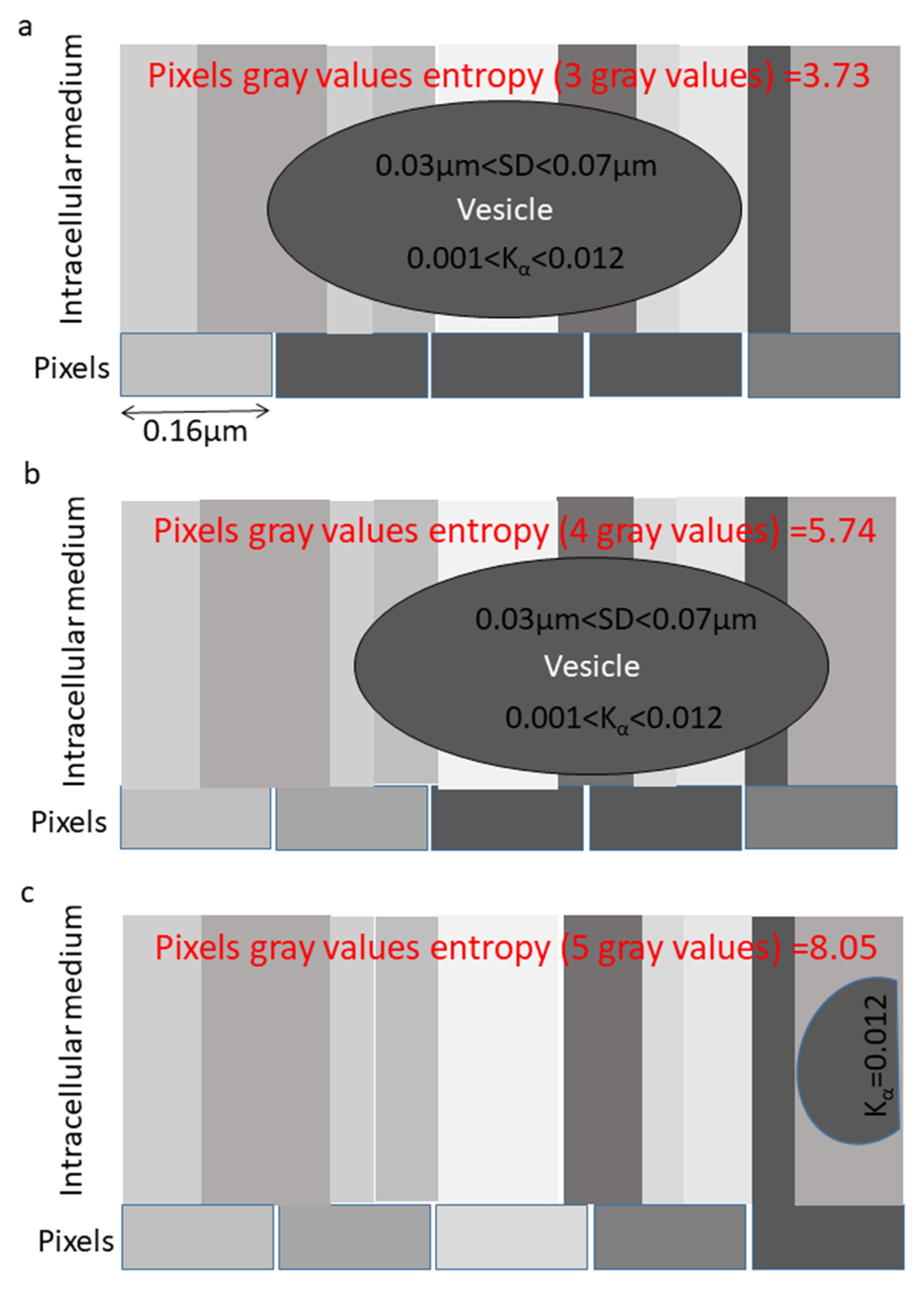
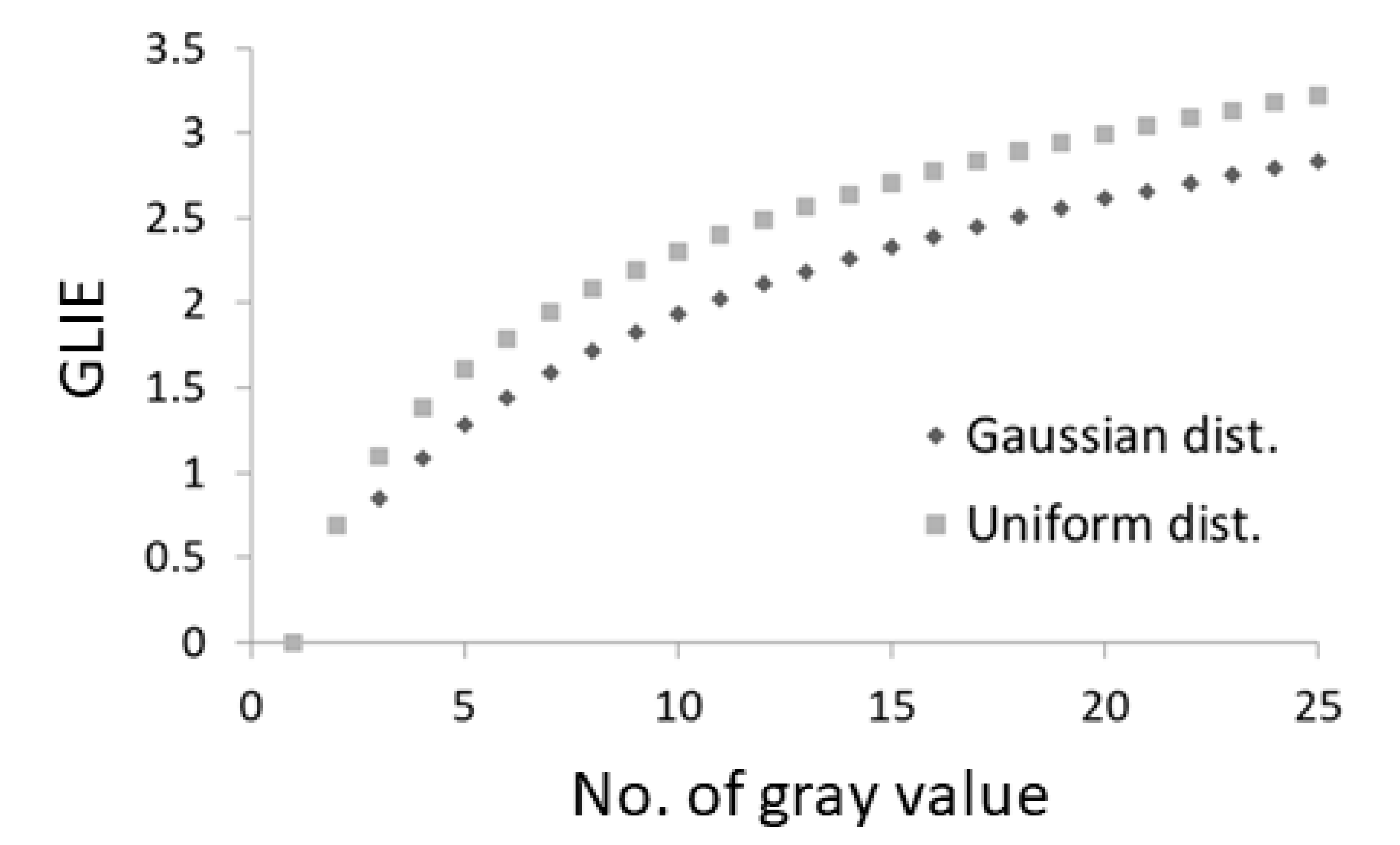
3.1. Gray Level Information Entropy (GLIE) Is Sensitive to the Motion of Intracellular Particles

Information entropy, E , can be calculated for the intensity distribution across the pixels of an image. Such entropy expresses the homogeneity of the inspected medium. The scale of changes in entropy is logarithmic due to the entropy function ( E = P i L n ( P i ) , where P i is the probability of occurrence of an intensity, i, and summation is over all intensity values).
Here, we focus on microscopy imaging of the interior of a cell in order to characterize the motion of intracellular particles. Such motion may produce pronounced fluctuations in the homogeneity and information entropy obtained from the intensity of relevant pixels. Such fluctuations depend on the size of the particles, their diffusivity and the pixel size.
For illustrations, we provide an example of a simple case of a particle undergoing a random walk in a homogeneous medium. The particle is captured by five pixels, as illustrated in Figure 1. In this situation, the particle motion will influence the readout intensity of specific pixels as follows. When the particle is located at the center (Figure 1a), the five intensities of the pixels will produce only two different gray levels. Accordingly, the information entropy calculated for the readout of the five pixels, is E = 1.43 . When the particle moves about 0.25 pixel-length from the center (Figure 1b), the intensity of the five pixels will now produce four different gray values, and E = 5.47 . When the particle moves about 0.5 pixel-length from the center (Figure 1c), the five intensities of the five pixels will produce now three different gray levels, and E = 3.44 . Thus, in this example the information entropy value of the five pixels ( E )   is fluctuating considerably between 1.43 and 5.74 due to the particle’s motion.
Next we consider a more realistic and complicated example of the motion of an intracellular particle (Figure 2). Here, the pixel width is taken as 0.16 μm (as in our experimental system) and the particle diameter is considered to be ~0.48 μm. This is a common (diffraction-limited) size of small intracellular entities, such as vesicles or sub-micron organelles [30]. Diffusivity of intracellular vesicles was measured to be 0.012 μm2/sec in normal cells (i.e., Jurkat cells with their normal metabolic activity) and 0.001 μm2/sec in ATP-depleted cells (with no mechanical work and only thermal agitation) [4]. We next consider a time lag of 0.2 s for inspecting the particle motion (as the time lag used in our experimental setup, which fits the time scale for intracellular active diffusion > 0.1 s). Accordingly, for a single time lag, the standard deviation (SD) of the Probability Density Function (PDF) of translocations of the particle is 0.07 μm in a normal cell and 0.03 μm for a particle in a cell after ATP-depletion. Thus, most of the translocations of the intracellular particle under ATP-depletion conditions are much smaller than the adjacent pixel length of 0.16 μm. The translocations become more comparable to the pixel size when considering a normal active cell.
The heterogeneity of the intracellular particle surrounding is expected to affect the relative information entropy in pixels that capture the particle vs. pixels that capture only the surrounding. Pixels that capture the particle will tend to have more homogenous intensity readouts and thus a relatively lower E values (Figure 2a). We can consider three principle locations of the intracellular particle. First, the particle is located at the center of five capturing pixels (Figure 2a). This yields three different gray levels, and E = 3.73 . Second, the particle moves about 0.5 pixel-length from the center (Figure 2b). The related five pixels produce four different gray levels, and E = 5.74 . Third, the particle is undergoing a large non-equilibrium translocation and is now almost out of the range of the related pixels (Figure 2c). The five capturing pixels now yield five different gray levels, and E = 8.05 .
Following this example, the particle motion could translate to corresponding changes in the information entropy values at the relevant pixels. For employing this technique to study the motion of intracellular particles, it is important to choose the appropriate number of capturing pixels according to the particle size and motion in order to generate maximal fluctuations in E . As an example, increasing the number of capturing pixels from five to seven in the example of Figure 2 yields fluctuations in E between 8.63 and 13.62. This range represents possible changes of up to 58% in E, and is relatively smaller than the corresponding range for five capturing pixels (of 116%). Increasing the number of capturing pixels will further decrease the relative fluctuation range of E .
A moving particle may create a change in the gray levels of its capturing pixels when it either protrudes into a neighboring pixel or withdraws from a capturing pixel (see example in the Figure 2b). This change is maximal when the particle moves to cover about 50% of a pixel. If the moving particle covers less than 50% of a pixel due to a small movement (and accordingly, more than 50% of the pixel on the opposite side), the gray levels and information entropy associated with those pixels are less likely to change. Given that, we can estimate the probability of that particle to translocate to a distance around half a pixel. We consider a translocation of 0.4–0.6 of a pixel length (here, 0.064–0.096 μm) in a normal active cell, for which the SD of translocation is 0.07 μm. In contrast, in an ATP-depleted cell the SD of translocations is 0.03 μm. This yields estimated probabilities of 0.095 for a normal active cell, in comparison to 0.015 for an ATP-depleted cell (see detailed calculations in Supplementary Materials Table S1). These probabilities reflect the higher occurrence rate of larger fluctuation in E due to the particle translocations in an active cell, relative to an ATP-depleted cell. Large non-equilibrium translocations of the particle that takes place in active cells and the corresponding large change in E (Figure 2c) are not expected to occur in ATP-depleted cells. Accordingly, we expect that fluctuations in E will be more pronounced in normal, active cells relative to ATP-depleted cells. Thus, parameters based on fluctuations in E of specific pixels could be utilized to detect and study intracellular mechanical activity.
Intracellular liquid–liquid phase separation is a process by which specific cellular material form pronounced complexes, such as nucleoli, condensates, etc. [31,32]. In mechanically active cells, intracellular liquid–liquid phase separation is reduced [6,33]. This may facilitate higher homogeneity of the intracellular content. More homogeny in the intracellular medium will result in average lower values of E . In this case, the fluctuations in E tend to be more pronounced due to the logarithmic nature of the entropy function (Figure 3). Therefore, in cells that are more mechanically active, fluctuations of E will be higher due to a synergic effect: an increase in the dynamics of intracellular particles, combined with an increase in the homogeneity of the intracellular content.

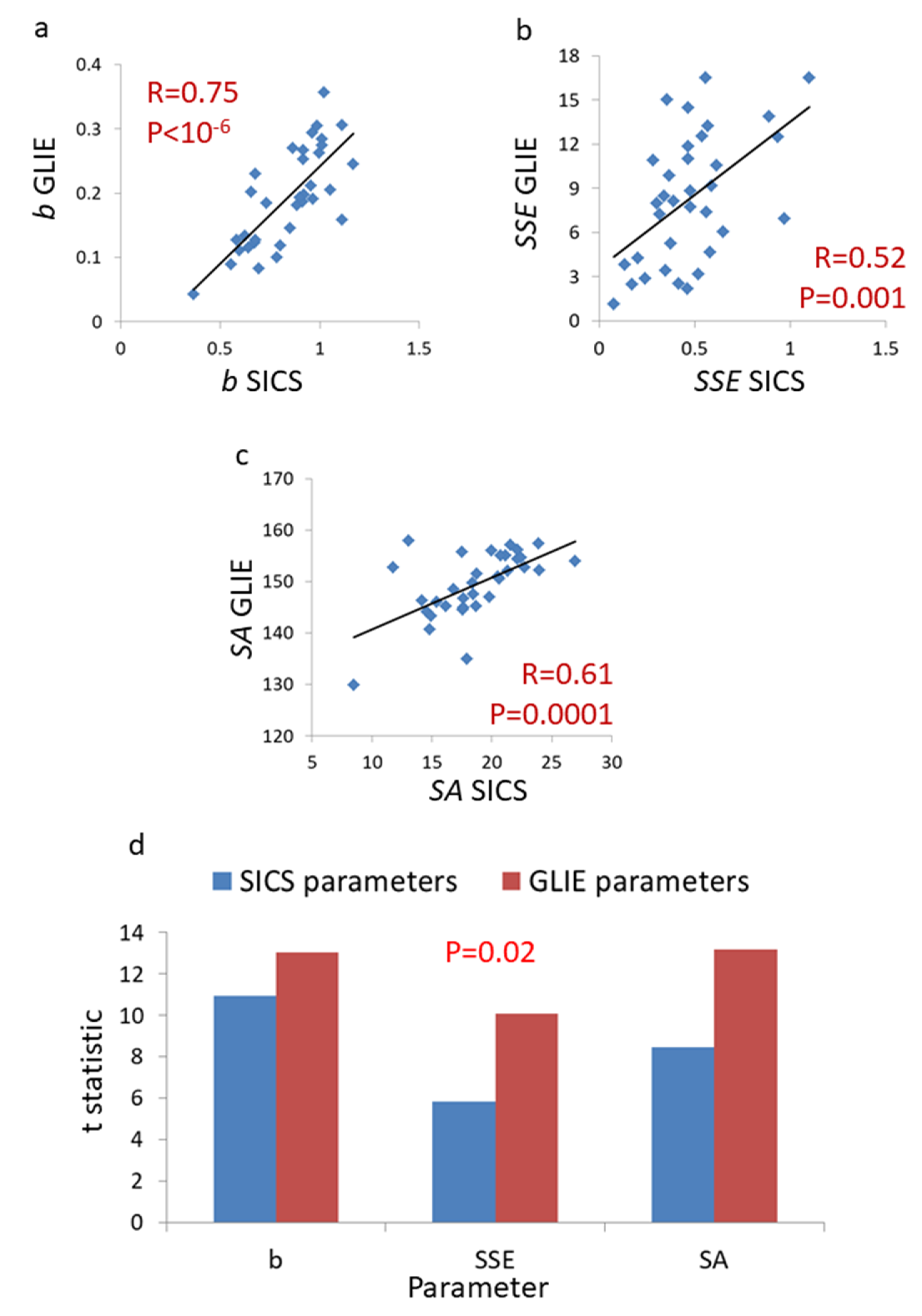
3.2. Comparing Pixel Gray-Levels Information Entropy (GLIE) Fluctuations and Spatial Image Correlation Spectroscopy (SICS) Fluctuations in Live Jurkat Cells before and after ATP Depletion

In the following section we test the ability of the proposed GLIE analysis to detect non-equilibrium mechanical activity in live cells. This is compared to the results in these cells after ATP depletion. The results of cell dynamics from GLIE fluctuation analysis were further compared to the results of cell dynamics, using the established tool of ICS analysis [29]. ICS analysis is based on analyzing spatial and temporal correlations of pixel intensities in a time series of images. When the spatial correlations (SICS) of each of the time-dependent images are also correlated in time, the dynamics of the related structures could be elucidated [29]. We studied fluctuations of GLIE or SICS by Amplitude Spectral Density (ASD) analysis and a power fit of the ASD results.
We conducted live cell imaging of Jurkat T lymphocytes. The label-free cells were imaged 200 times with a 0.2 s interval. We studied a region of interest (ROI) of 50 × 50 pixels at the center of each measured cell, and conducted GLIE and SICS fluctuations analysis within (Figure 4a). For SICS analyses, results of the six lowest spatial lags from the horizontal and from the vertical axes were excluded because they were significantly influenced by PSF-dependent correlations. For the remaining 18 lags of each dimension, we conducted DFT analysis for each lag of the time-dependent correlations. The calculated DFT amplitudes of the 18 × 2 lags were then averaged to get the ASD results of that cell and also the related power fit parameters of that spectrum. The average ASD results from the SICS analysis of all the cells under each condition (before and after ATP depletion) are presented in Figure 4b.
The GLIE fluctuation analysis is further demonstrated in Figure 5a–d. The 50 × 50 pixels ROI of each cell was further divided into 100 units of 5 × 5 pixels (Figure 5b), in accordance with the conclusions in the previous section. In each 5 × 5 unit, GLIE values were calculated for each of the 200 time points (Figure 5d). Next, the 200 time-dependent GLIE results of each unit of 5 × 5 pixels were analyzed by DFT. Averaged amplitudes of all 100 (5 × 5 pixels) units for each frequency were determined to define the ASD results of that cell regarding GLIE fluctuations. The average ASD results from the GLIE analysis of all the cells under each condition (before and after ATP depletion) are presented in Figure 4c.
The ASD results (Figure 4b,c) show that the amplitudes of SICS and GLIE fluctuations have similar patterns and are both higher in normal active cells, as compared to these cells after ATP depletion. The compatibility of power-fit regressions to these ASD patterns is high according to the R-values presented in Figure 4b,c. These high compatibilities of power-fit formulas to the ASD results are not surprising, since multiple analytical models of Brownian and anomalous diffusion were found to match the general formula: A m p l i t u d e   ( f , ) = D f 0.5 β , where   f represents the frequency, β represents the power of diffusion and D represents a constant that relates to Kα [19,20,21]. The power-fit ( A m p l i t u d e = a F r e q u e n c y b ) parameters a, b and Sum of Squared estimate of Errors (SSE), as well as the parameter Sum of Amplitudes (SA), were defined and calculated in each analysis (SICS fluctuations or GLIE fluctuations) for each cell and each condition (Figure 6). Apart from the a parameters in the SICS fluctuation analysis, all other parameters were significantly higher in live cells before ATP depletion, as compared to the values in the same cells after ATP depletion.
As previously suggested, PSD or ASD analyses can serve for characterizing intracellular dynamics, and relate to the Mean Squared Displacement (MSD) equation; M S D = K α Δ t α , where K α represents the diffusion coefficient, Δ t represents the time lag and α represents the power of diffusion [20]. Specifically, the a parameter is related to Kα—the diffusion coefficient; the b parameter is related to α—the power of the diffusion. Like α, the parameter b also increases by introducing mechanical work to the cell and a break in ergodicity. The SSE parameter also increases by adding mechanical work and a break in ergodicity. The SA parameter relates to the general dynamics in the measured system. As expected according to these relations, we observe higher parameter values obtained in active cells that produce significant amount of mechanical work in comparison to cells after ATP depletion, in which no mechanical work is produced.
We observe significant correlations between SICS-based parameters and their corresponding GLIE-based parameters (Figure 7). These correlations establish the ability of GLIE-based parameters to characterize aspects of intracellular dynamics. Based on t-statistics (Figure 7d), GLIE-based parameters seem to provide a significantly higher discrimination power between conditions of normal cellular activity and ATP depletion.
The advantage of GLIE-based parameters in the detection of intracellular dynamics due to mechanical work may stem from the intracellular medium becoming more homogenous under such conditions [6]. This is reflected by the average GLIE values that are lower in these cells (Figure 8). Due to the fact that GLIE is a logarithmic function, lower average GLIE values make GLIE fluctuations more pronounced (Figure 3). Hence, the combined effect of an increase in intracellular motion and an increase in intracellular homogeneity enables the resultant high GLIE fluctuations. This increases the sensitivity of our approach to intracellular mechanical work and related dynamics (Figure 7d).
The a parameter (which relates to Kα) is expected to be higher in active cells, as compared to ATP-depleted cells [4,6]. Therefore, the relatively lower a parameter results in active cells found by our SICS analysis (Figure 6a) needs further consideration. These unexpected lower a parameter values are probably due to artifactual lowering of this parameter as a result of a significant degree of mismatch between the ASD values and their adjusted power fit under this condition. We further discuss this subject in the Supplementary Materials. When using GLIE-based fluctuation analysis, this issue is resolved due to the lower average GLIE values in the normal active cells (Figure 8). Higher homogeneity in active cells causes a further increase in a values. This increase compensates for the artifactual lowering of a values through the power fit. As a result, when using GLIE fluctuation analysis, a values are higher in cells before ATP depletion than after ATP depletion.

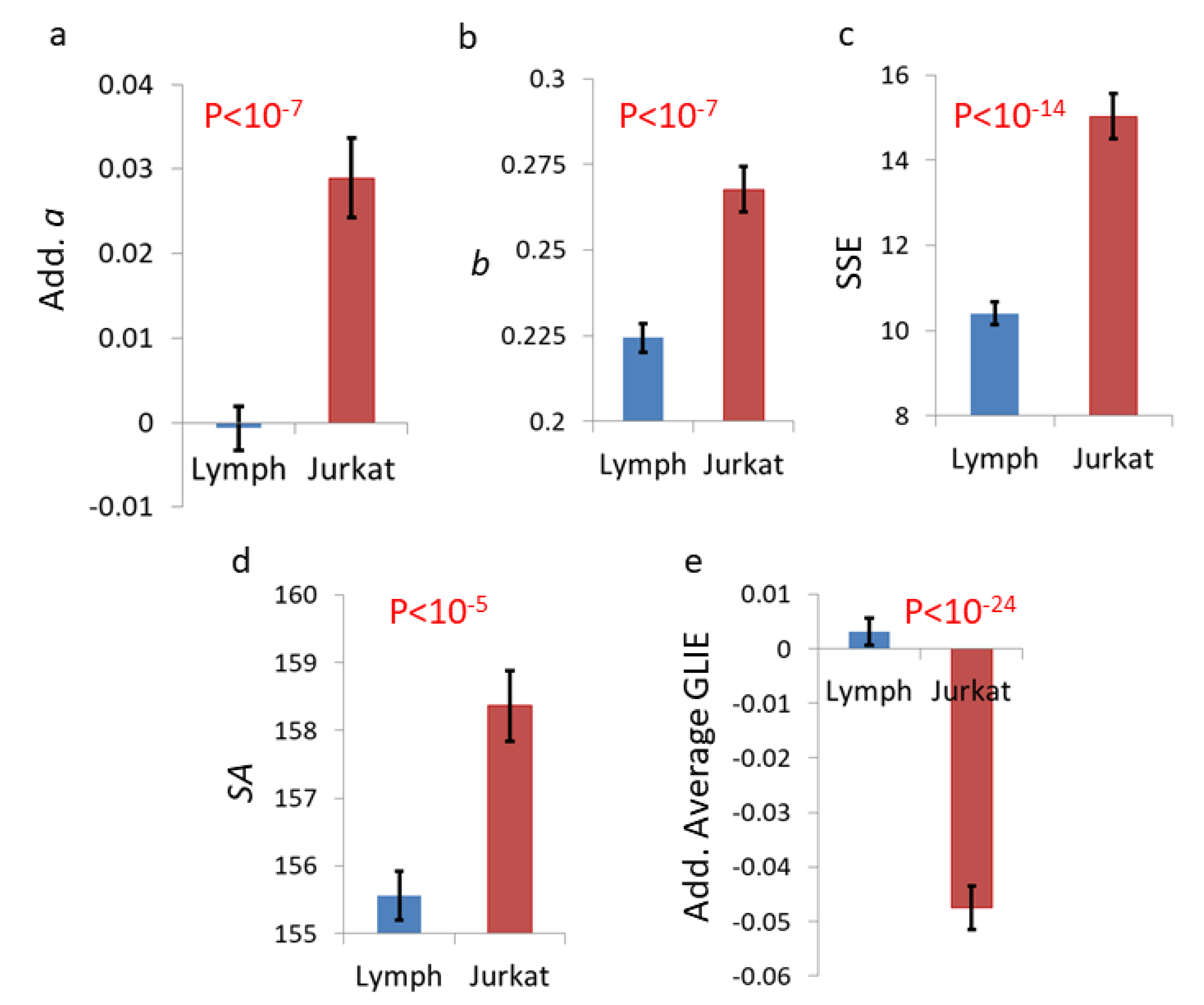
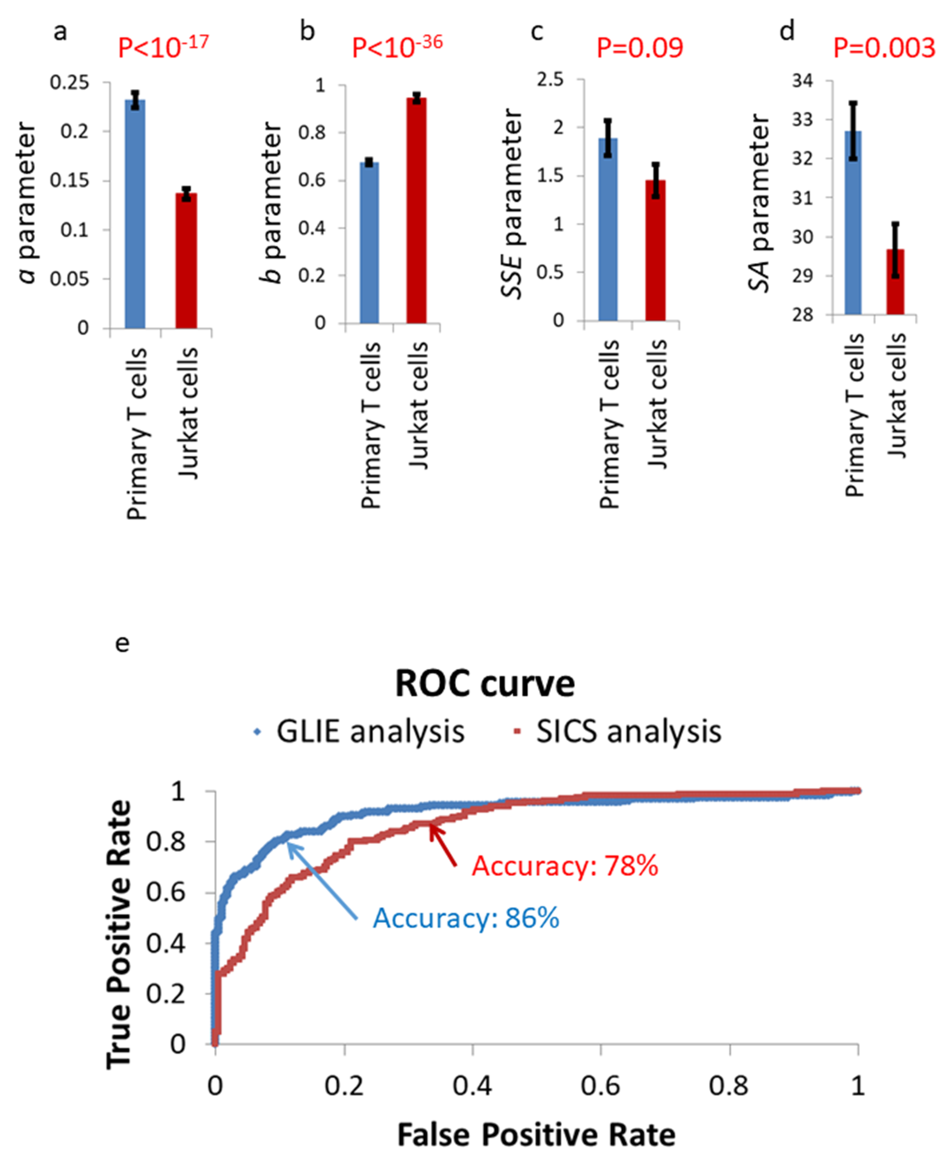
3.3. Comparing GLIE Fluctuations in Live Jurkat and Primary T Cells

Intracellular mechanical work and motion are known to be higher in malignant cells [4,9]. Thus, we decided to test whether the high sensitivity of our GLIE-based analysis to intracellular mechanical work could differentiate between benign and malignant cells.
Using the outline in Section 3.2 for GLIE analysis, we measured 219 primary T cells and 161 malignant Jurkat cells. Because primary T cells are a little smaller than Jurkat cells, we utilized for this experiment ROI’s of 40 × 40 pixels at the center of each measured cell. Figure 9 shows typical images of a primary T cell and a Jurkat cell, with the 40 × 40 pixels ROIs for GLIE calculation at their center.
In this experiment we kept the microscope light intensity constant for both types of cells. Still, the average gray levels of pixels in the ROIs were significantly different between these two types of cells (Figure 9; p < 10−51). Malignant cells are known to differ from their counterpart benign cells in their refractive index [34] and density [35]. Thus, it is expected that the same illumination will produce different intensities of received light (and detected gray levels) for the benign and malignant cells. To evaluate the possible impact of this difference on the GLIE fluctuation parameters, we analyzed the correlation between the average gray level and each of the GLIE fluctuation parameters in both types of the populations of primary T cells and malignant Jurkat cells. We found that in both type of cells there was no correlation between the average gray level and the parameters b, SSE and SA. Only a and the average GLIE showed correlation to the average gray level in primary T cells and not in Jurkat cells (Figure 10). Higher illumination light intensity is expected to increase the distribution of gray levels in the image. This expected correlation between light intensity (or average gray value) and the number of gray values in the measurement unit of 5 × 5 pixels could be clearly demonstrated in primary T cells (R = 0.56, p < 10−19) but not in malignant Jurkat cells (R = 0.06, p = 0.43). We hypothesize that in the malignant Jurkat cells other structural or organization processes (such as the degree of fractal dimension of intracellular content [36]) are more dominant in determining the distribution of gray levels in the pixel’s measurement unit than light intensity. Because the number of gray values is clearly related to GLIE (Figure 3), a correlation between average gray level and average GLIE could be expected and demonstrated in primary T cells, yet not in malignant Jurkat cells (Figure 10a,b). The negative correlation between average GLIE and a parameter (Figure 10c,d) that was mentioned previously (due to the logarithmic GLIE function) create the negative correlation between the average gray level and the a parameter in primary T cells (Figure 10e).
The impact of light intensity (or average gray level) on the average GLIE and a parameters in primary T cells dictates adjustment of these parameters in order to neutralize the effect of different light intensities. Figure 11 illustrates a neutralization procedure of the light intensity effect through adjusting the average GLIE and a parameters. This neutralization procedure is based on first determining the regression function in primary T cells for these two parameters from the average gray level. Then, we calculate the difference between the measured value of the parameter and its predicted value according to the regression function.
Calculating the adjusted a parameter (adj. a) and other GLIE fluctuation parameters (b, SSE and SA) in primary T cells and in Jurkat malignant cells reveals that the values of these parameters are much higher in malignant cells (as shown in Figure 12). On the other hand, adjusted average GLIE values were lower in the malignant cells. The higher mechanical work and dynamics in malignant cells probably resulted in more intracellular homogeneity, lower adjusted GLIE (adj. GLIE) values and higher GLIE fluctuation parameters: adj. a, b, SSE and SA. Differences in structural parameters or insufficient normalization of different light intensities may also influence the adjusted average GLIE values.
When analyzing the difference between primary T lymphocytes and Jurkat cells according to the corresponding SICS analysis parameters, the obtained results are less consistent. As can be seen in Figure 13, while b parameter is significantly higher in Jurkat cells, all other parameters (namely a, SSE and SA) are all lower in these cells.
Utilizing GLIE or SICS parameters may enable an accurate differentiation between primary T cells and malignant (Jurkat) T cells on the basis of multiple, single cell examinations. When analyzed by a binary logistic regression, we found a discrimination power or AUC (Area Under Receiver-Operating-Characteristic (ROC) Curve) of 0.92 for GLIE parameters and 0.86 for SICS parameters (see ROC curve in Figure 13e). The percentage of correct classifications was 86% for GLIE parameters and 78% for SICS parameters (with a classification cutoff of 0.5). The same set of data of Jurkat and lymphocytes results (described in Figure 12) was used for both training and testing of the classifier. Following these results, it can be seen that GLIE parameters better differentiate between primary T cells and malignant Jurkat cells. Notably, in a clinical setup for malignancy diagnosis, typically hundreds of cells are examined. Thus, the AUC of 0.92 and percentage of correct classifications of 86% for a single cell examination will produce much higher discriminating results when more cells are examined. For example, moderately increasing the number of cells from 1 to 10 and averaging the results provides an AUC of 0.997 and 95% of correct classifications.
It was important to verify if other physiological condition other than malignancy such as activation or proliferation and differentiation could also raise GLIE fluctuations parameter values. To verify this subject primary T cells were stimulated with human anti CD3 or with PMA while incubated on the microscope stage (as further detailed in the Materials and Methods section). The results of GLIE fluctuations parameters in these cells before and after stimulation with anti-CD3 or stimulation with PMA are summarized in Figure 14.
As can be seen in Figure 14, GLIE parameters (except for SSE) were significantly lower after both cellular stimulations. For control, GLIE fluctuation parameters were evaluated in fixed Jurkat cell. Their results were very low even in comparison to primary T cells (Supplementary Materials Figure S2).
The results so far suggest that GLIE fluctuation parameters could accurately differentiate cellular malignancy from a wide range of cellular physiological conditions that include activation, proliferation and differentiation.

4. Discussion

Information entropy or homogeneity changes in an inspected medium can reflect the motion of particles within that medium. For optimal sensitivity of these measures, the right length- and time-scales should be chosen for inspection, such that they suit the particle size and expected motion. To illustrate this principle, we first provided examples of particle motion in homogeneous and non-homogeneous media. Theoretical analysis of a non-homogeneous medium suggests ways to improve the characterization of live cells under typical experimental conditions. Specifically, we considered parameters such as the pixel size, the size of the particles under study, the number of pixels used in analysis, the particle diffusivity and the time-lag between acquisitions. Evaluation of the motion of large intracellular particles (such as vesicles or organelles) is particularly important for study of the cell physiology. These large particles are embedded within the actin cytoskeletal mesh, and, accordingly, their motion reflects the motion of the cell cytoskeleton and the expenditure of intracellular mechanical work. As shown, fluctuations in the information entropy of selected pixels can reflect dynamics of the inspected medium in live cells.
An important and inherent advantage of GLIE analysis is its sensitivity to intracellular mechanical work, which increases the homogeneity of the cell medium. In a more active and dynamic cell, the partition of the cell’s constituents is reduced [6,33], and so is the heterogeneity of the pixel gray levels and the average value of GLIE (Figure 8). Lower average GLIE values enable augmentation of momentary GLIE variation due to the logarithmic GLIE function (in Figure 3, the derivatives of GLIE curve are negatively correlated to GLIE values). This contributes to higher GLIE fluctuations in mechanically active cells. The application of ASD analysis to GLIE fluctuation, with the aid of power-fit parameters, enables the characterization of the cell’s dynamic, including its constituents of diffusion coefficient, degree of anomalous diffusion and mechanical work.
Cellular dynamics is affected by both passive factors (as elasticity or viscosity) and active ATP-dependent intracellular mechanical work. A sensitive tool to evaluate intracellular dynamics, along with its different contributing factors, should be very useful to study important cellular pathophysiological conditions. Such conditions may relate to energy imbalance and change of intracellular rheological factors. Cell conditions that effect ATP metabolism as cellular ischemia [37] or mitochondrial dysfunction [4,8] were found to reduce intracellular mechanical work and intracellular dynamics. Mitochondrial dysfunction states relate to a wide area of clinical abnormalities from neurodegenerative diseases (like Alzheimer’s disease, Parkinson’s disease, amyotrophic lateral sclerosis, Huntington’s disease) [38,39], aging [40], autism [41], chronic fatigue syndrome [42], cancer [43] and skin diseases [44] to insulin resistance [45] and more. Accordingly, it is important to acquire a sensitive biophysical tool which will enable the detailed characterization of these influential pathophysiological conditions.
In our results, we further demonstrated the ability of GLIE fluctuation parameters to distinguish a cellular state of mitochondrial dysfunction and ATP depletion. GLIE fluctuations parameters a, b, SSE and SA were all significantly higher in the normal active cells, as compared to the results in these cells after ATP depletion (Figure 6b). For validation of these results, we further analyzed the dynamics of these cells by using SICS fluctuation analysis (Figure 6a). As expected, the results from these two methods were correlated. Still, the GLIE fluctuations analysis method provided significantly more discriminating power for differentiating these two cellular metabolic states (Figure 7d).
Malignant cells have high extent of intracellular mechanical work accompanied with low values of intracellular elasticity and viscosity [4]. Thus, we anticipated high values of GLIE fluctuation parameters in these cells. This concept was experimentally tested in two models of lymphocytes. The first are malignant Jurkat cells. These cells are derived from a human cell line source, which originated from the peripheral blood of a T-cell leukemia patient. These cells were compared to primary T cells as a second model of benign human lymphocytes (see Material and Methods). Although the microscope illumination was the same during the experiment, the received light intensity and average gray level in these two cells types were different. This is probably due to different optical characteristics of these two types of cells. Since the parameters a and average GLIE were found to be sensitive to the illuminating light intensity, they had to be adjusted in order to neutralize the effect of the difference in light intensity (see Section 3.3 in Results). As expected, GLIE fluctuation parameters b, SSE and SA, as well as the adjusted parameter a, were all found to be higher in Jurkat malignant cells in comparison to primary T cells (Figure 12a–d). Malignant cells, with their high intracellular dynamics and mechanical work, are expected to have more homogeneous content. Indeed, the average adjusted GLIE values were lower in malignant Jurkat cells relative to benign primary T cells (Figure 12e).
Malignant and benign lymphocytes look generally similar (e.g., in Figure 9). Thus, a pathologist faces a substantial clinical challenge to accurately differentiate these two types of cells according to morphology-based criteria. For that, an accessory biophysical (rather than morphological-based) diagnostic tool may be beneficial. We present an initial evaluation of the accuracy of GLIE fluctuation parameters in differentiating malignant Jurkat cells from primary T cells, utilizing binary logistic regression with a ROC curve (Figure 13e). The percentage of correct classifications for single malignant cell detection (in a single cell examination) was 86% and AUC 0.92. This accuracy may seem relatively low, but it has to be considered in the appropriate clinical setup of malignancy investigation where usually hundreds of suspected cells are examined. Under such conditions, the basic accuracy level for a single cell examination will rise considerably. For instance, the modest increase in the number of the examined cells to 10 similar cells increases the percentage of correct classifications to 95% and AUC to 0.997.
PMA is a Protein Kinas C (PKC) activator that induces cell proliferation and differentiation. Anti-CD3ε antibodies are known activators of T cells. Applying either of these conditions lowered GLIE fluctuation parameters in primary T cells. It is possible that the high dynamics in malignant cells that is reflected by the high GLIE fluctuations is related to the low differentiation state of these cells. PMA, which causes the primary T cells to differentiate, may have lowered GLIE fluctuations in these cells. This encouraging result indicates that GLIE fluctuation parameters could accurately diagnose malignancy across a wide range of physiological conditions that relate to cell activation, proliferation or differentiation.
GLIE fluctuation analysis utilizing ASD and power-fit parameters requires a simple experimental setup of regular bright field microscope and label-free cell samples. The analysis could be easily automated. It further provides quick results that reflect biophysical cell parameters as intracellular motion and homogeneity. Thus, this analysis enables the study of cellular conditions of energetic imbalance as mitochondrial dysfunction and enables the accurate differentiation of malignant from benign lymphocytes. Further development of this tool may assist in research and clinical evaluation and diagnostics of malignancy and possibly other relevant clinical pathologies.

Supplementary Materials

The following are available online at https://www.mdpi.com/2076-3417/10/24/8894/s1. Table S1: Parameters of intracellular particle translocations. Figure S1: A gap between ASD values of SICS fluctuation analysis and their power-fit result is artifactually lowering a parameter values. (a) ASD of SICS fluctuations in Jurkat cells (n = 34) before ATP depletion and in those cells after ATP depletion. Power-fit regression lines are highlighted. (b) The correlation between b and a parameters of SICS fluctuation analysis in the Jurkat cells before and after ATP depletion. In the cells before ATP depletion the correlation is significant and R- and p-value of that correlation are presented. Figure S2: GLIE fluctuations in fixed Jurkat cells and in live primary T cells. (a) Average DFT results of GLIE fluctuations in fixed Jurkat cells and live primary T cells. (b) The results of (a) in the frequency range of 0.5–2.5 Hz. (c) Average R2 of the power fit in fixed Jurkat cells and in live primary T cells. GLIE fluctuation parameters: a (d), b (e), SSE (f) and SA (g) in fixed Jurkat cells and in live primary T cells. Error bars in are SEM. p-values are presented in the corresponding panels.

Author Contributions

Conceptualization, I.W. and E.S.; methodology, I.W. and E.S.; validation, I.W.; formal analysis, I.W., O.Y.; investigation, I.W.; resources, E.S.; data curation, I.W.; writing—original draft preparation, I.W.; writing—review and editing, E.S.; visualization, I.W.; supervision, E.S.; funding acquisition, E.S. All authors have read and agreed to the published version of the manuscript.

Funding

This research was funded by the ISF, grant number 1761/17.

Acknowledgments

We thank Anat Globerson Levin from the Sourasky medical center in Tel-Aviv for providing us with human primary T cells. We thank Yaron Hakuk from the The Biophysical Interdisciplinary Schottenstein Center for the Research and Technology of the Cellome, Physics Department, Bar Ilan University, for helping us with part of the Matlab codes.

Conflicts of Interest

The authors declare no conflict of interest. The funders had no role in the design of the study; in the collection, analyses or interpretation of data; in the writing of the manuscript; or in the decision to publish the results.

References

  1. Vale, R.D. The Molecular Motor Toolbox for Intracellular Transport. Cell 2003, 112, 467–480. [Google Scholar] [CrossRef] [Green Version]
  2. Manfred, S.; Woehlke, G. Molecular Motors. Nature 2003, 422, 45–55. [Google Scholar] [CrossRef]
  3. Brangwynne, C.P.; Koenderink, G.H.; Mackintosh, F.C.; Weitz, D.A. Intracellular transport by active diffusion. Trends Cell Biol. 2009, 19, 423–427. [Google Scholar] [CrossRef] [PubMed]
  4. Guo, M.; Ehrlicher, A.J.; Jensen, M.H.; Renz, M.; Moore, J.R.; Goldman, R.D.; Lippincott-Schwartz, J.; Mackintosh, F.C.; Weitz, D.A. Probing the Stochastic, Motor-Driven Properties of the Cytoplasm Using Force Spectrum Microscopy. Cell 2014, 158, 822–832. [Google Scholar] [CrossRef] [PubMed] [Green Version]
  5. Ishijima, A.; Kojima, H.; Funatsu, T.; Tokunaga, M.; Higuchi, H.; Tanaka, H.; Yanagida, T. Simultaneous Observation of Individual ATPase and Mechanical Events by a Single Myosin Molecule during Interaction with Actin. Cell 1998, 92, 161–171. [Google Scholar] [CrossRef] [Green Version]
  6. Wohl, I.; Sherman, E. ATP-Dependent Diffusion Entropy and Homogeneity in Living Cells. Entropy 2019, 21, 962. [Google Scholar] [CrossRef] [Green Version]
  7. Tuvia, S.; Levin, S.; Bitler, A.; Korenstein, R. Mechanical Fluctuations of the Membrane–Skeleton Are Dependent on F-Actin ATPase in Human Erythrocytes. J. Cell Biol. 1998, 141, 1551–1561. [Google Scholar] [CrossRef]
  8. Wohl, I.; Zurgil, N.; Hakuk, Y.; Deutsch, M.S.A.M. In Situ Evaluation of Physiological Activity and Mitochondrial Dysfunction via Novo Label-Free Measures Based on Fluctuation of Image Gray Values. J. Anal. Bioanal. Tech. 2016, 7, 308. [Google Scholar] [CrossRef] [Green Version]
  9. Lau, A.W.C.; Hoffman, B.D.; Davies, A.; Crocker, J.C.; Lubensky, T.C. Microrheology, Stress Fluctuations, and Active Behavior of Living Cells. Phys. Rev. Lett. 2003, 91, 198101. [Google Scholar] [CrossRef] [Green Version]
  10. Li, Y.; Schnekenburger, J.; Duits, M.H.G. Intracellular particle tracking as a tool for tumor cell characterization. J. Biomed. Opt. 2009, 14, 064005. [Google Scholar] [CrossRef]
  11. Suh, J.; Wirtz, D.; Hanes, J. Real-Time Intracellular Transport of Gene Nanocarriers Studied by Multiple Particle Tracking. Biotechnol. Prog. 2008, 20, 598–602. [Google Scholar] [CrossRef] [PubMed]
  12. Reverey, J.F.; Jeon, J.-H.; Bao, H.; Leippe, M.; Metzler, R.; Selhuber-Unkel, C. Superdiffusion dominates intracellular particle motion in the supercrowded cytoplasm of pathogenic Acanthamoeba castellanii. Sci. Rep. 2015, 5, srep11690. [Google Scholar] [CrossRef] [PubMed] [Green Version]
  13. Zam, A.; Kolios, M.C. Measuring intracellular motion in cancer cell using optical coherence tomography. Dyn. Fluct. Biomed. Photonics XIII 2016, 9707, 97070. [Google Scholar] [CrossRef]
  14. Nicolay, K.; Braun, K.P.J.; De Graaf, R.A.; Dijkhuizen, R.M.; Kruiskamp, M.J. Diffusion NMR spectroscopy. NMR Biomed. 2001, 14, 94–111. [Google Scholar] [CrossRef] [PubMed]
  15. Wohl, I.; Zurgil, N.; Hakuk, Y.; Sobolev, M.; Bar-On, Z.E. Fluctuation of Information Entropy Measures in Cell Image. Entropy 2017, 19, 565. [Google Scholar] [CrossRef] [Green Version]
  16. Wohl, I.; Zurgil, N.; Hakuk, Y.; Sobolev, M.; Galmidi, M.; Deutsch, M. In situ label-free static cytometry by monitoring spatiotemporal fluctuations of image gray values. J. Biomed. Opt. 2015, 20, 105013. [Google Scholar] [CrossRef]
  17. Jeon, J.-H.; Tejedor, V.; Burov, S.; Barkai, E.; Selhuber-Unkel, C.; Berg-Sørensen, K.; Oddershede, L.B.; Metzler, R. In VivoAnomalous Diffusion and Weak Ergodicity Breaking of Lipid Granules. Phys. Rev. Lett. 2011, 106, 048103. [Google Scholar] [CrossRef] [Green Version]
  18. Regner, B.M.; Vučinić, D.; Domnisoru, C.; Bartol, T.M.; Hetzer, M.W.; Tartakovsky, D.M.; Sejnowski, T.J. Anomalous diffusion of single particles in cytoplasm. Biophys. J. 2013, 104, 1652–1660. [Google Scholar] [CrossRef] [Green Version]
  19. Krapf, D.; Marinari, E.; Metzler, R.; Oshanin, G.; Xu, X.; Squarcini, A. Power spectral density of a single Brownian trajectory: What one can and cannot learn from it. New J. Phys. 2018, 20, 023029. [Google Scholar] [CrossRef]
  20. Krapf, D.; Lukat, N.; Marinari, E.; Metzler, R.; Oshanin, G.; Selhuber-Unkel, C.; Squarcini, A.; Stadler, L.; Weiss, M.; Xu, X. Spectral Content of a Single Non-Brownian Trajectory. Phys. Rev. X 2019, 9, 011019. [Google Scholar] [CrossRef] [Green Version]
  21. Sposini, V.; Metzler, R.; Oshanin, G. Single-trajectory spectral analysis of scaled Brownian motion. New J. Phys. 2019, 21, 073043. [Google Scholar] [CrossRef]
  22. Pantic, I.; Pantic, S.; Paunovic, J. Aging Increases Nuclear Chromatin Entropy of Erythroid Precursor Cells in Mice Spleen Hematopoietic Tissue. Microsc. Microanal. 2012, 18, 1054–1059. [Google Scholar] [CrossRef] [PubMed]
  23. Pantic, I.; Pantic, S.; Basta-Jovanovic, G. Gray Level Co-Occurrence Matrix Texture Analysis of Germinal Center Light Zone Lymphocyte Nuclei: Physiology Viewpoint with Focus on Apoptosis. Microsc. Microanal. 2012, 18, 470–475. [Google Scholar] [CrossRef] [PubMed] [Green Version]
  24. Pantic, I.; Pantic, S. Germinal Center Texture Entropy as Possible Indicator of Humoral Immune Response: Immunophysiology Viewpoint. Mol. Imaging Biol. 2011, 14, 534–540. [Google Scholar] [CrossRef]
  25. De Arruda, P.F.F.; Gatti, M.; Junior, F.N.F.; De Arruda, J.G.F.; Moreira, R.D.; Junior, L.O.M.; De Arruda, L.F.; De Godoy, M.F. Quantification of fractal dimension and Shannon’s entropy in histological diagnosis of prostate cancer. BMC Clin. Pathol. 2013, 13, 6. [Google Scholar] [CrossRef]
  26. Chithra Devi, M.; Audithan, S. Analysis of different types of entropy measures for breast cancer diagnosis using ensemble classification. Biomed. Res. 2017, 28, 3182–3186. [Google Scholar]
  27. Li, N.; Ragheb, K.; Lawler, G.; Sturgis, J.; Rajwa, B.; Melendez, J.A.; Robinson, J.P. Mitochondrial Complex I Inhibitor Rotenone Induces Apoptosis through Enhancing Mitochondrial Reactive Oxygen Species Production. J. Biol. Chem. 2003, 278, 8516–8525. [Google Scholar] [CrossRef] [Green Version]
  28. Martin, J.A.; Martini, A.; Molinari, A.; Morgan, W.; Ramalingam, W.; Buckwalter, J.A.; McKinley, T.O. Mitochondrial electron transport and glycolysis are coupled in articular cartilage. Osteoarthr. Cartil. 2012, 20, 323–329. [Google Scholar] [CrossRef] [Green Version]
  29. Kolin, D.L.; Wiseman, P. Advances in Image Correlation Spectroscopy: Measuring Number Densities, Aggregation States, and Dynamics of Fluorescently labeled Macromolecules in Cells. Cell Biophys. 2007, 49, 141–164. [Google Scholar] [CrossRef]
  30. Tucher, C.; Bode, K.; Schiller, P.; Claßen, L.; Birr, C.; Souto-Carneiro, M.M.; Blank, N.; Lorenz, H.-M.; Schiller, M. Extracellular Vesicle Subtypes Released From Activated or Apoptotic T-Lymphocytes Carry a Specific and Stimulus-Dependent Protein Cargo. Front. Immunol. 2018, 9, 534. [Google Scholar] [CrossRef] [Green Version]
  31. Hyman, A.A.; Weber, C.A.; Jülicher, F. Liquid-Liquid Phase Separation in Biology. Annu. Rev. Cell Dev. Biol. 2014, 30, 39–58. [Google Scholar] [CrossRef] [PubMed] [Green Version]
  32. Brangwynne, C.P.; Tompa, P.; Pappu, R.V. Polymer physics of intracellular phase transitions. Nat. Phys. 2015, 11, 899–904. [Google Scholar] [CrossRef]
  33. Wohl, I.; Yakovian, O.; Razvag, Y.; Reches, M.; Sherman, E. Fast and synchronized fluctuations of cortical actin negatively correlate with nucleoli liquid–liquid phase separation in T cells. Eur. Biophys. J. 2020, 49, 1–15. [Google Scholar] [CrossRef] [PubMed]
  34. Choi, W.J.; Jeon, D.I.; Ahn, S.-G.; Yoon, J.-H.; Kim, S.; Lee, B.-H. Full-field optical coherence microscopy for identifying live cancer cells by quantitative measurement of refractive index distribution. Opt. Express 2010, 18, 23285–23295. [Google Scholar] [CrossRef]
  35. Phillips, K.G.; Velasco, C.R.; Li, J.; Kolatkar, A.; Luttgen, M.; Bethel, K.; Duggan, B.; Kuhn, P.; Mccarty, O.J.T. Optical Quantification of Cellular Mass, Volume, and Density of Circulating Tumor Cells Identified in an Ovarian Cancer Patient. Front. Oncol. 2012, 2, 72. [Google Scholar] [CrossRef] [Green Version]
  36. Dey, P.; Mohanty, S.K. Fractal dimensions of breast lesions on cytology smears. Diagn. Cytopathol. 2003, 29, 85–86. [Google Scholar] [CrossRef]
  37. Harkins, K.D.; Galons, J.-P.; Divijak, J.L.; Trouard, T.P. Changes in intracellular water diffusion and energetic metabolism in response to ischemia in perfused C6 rat glioma cells. Magn. Reson. Med. 2011, 66, 859–867. [Google Scholar] [CrossRef] [Green Version]
  38. Lin, M.T.; Beal, M.F. Mitochondrial dysfunction and oxidative stress in neurodegenerative diseases. Nat. Cell Biol. 2006, 443, 787–795. [Google Scholar] [CrossRef]
  39. Gibson, G.E.; Starkov, A.; Blass, J.P.; Ratan, R.R.; Beal, M.F. Cause and consequence: Mitochondrial dysfunction initiates and propagates neuronal dysfunction, neuronal death and behavioral abnormalities in age-associated neurodegenerative diseases. Biochim. et Biophys. Acta (BBA) Mol. Basis Dis. 2010, 1802, 122–134. [Google Scholar] [CrossRef] [Green Version]
  40. Wiley, C.D.; Velarde, M.C.; Lecot, P.; Liu, S.; Sarnoski, E.A.; Freund, A.; Shirakawa, K.; Lim, H.W.; Davis, S.S.; Ramanathan, A.; et al. Mitochondrial Dysfunction Induces Senescence with a Distinct Secretory Phenotype. Cell Metab. 2016, 23, 303–314. [Google Scholar] [CrossRef] [Green Version]
  41. Legido, A.; Jethva, R.; Goldenthal, M.J. Mitochondrial Dysfunction in Autism. Semin. Pediatr. Neurol. 2013, 20, 163–175. [Google Scholar] [CrossRef] [PubMed]
  42. Myhill, S.; Booth, N.E.; McLaren-Howard, J. Chronic fatigue syndrome and mitochondrial dysfunction. Int. J. Clin. Exp. Med. 2009, 2, 1–16. [Google Scholar] [PubMed]
  43. Pelicano, H.; Zhang, W.; Liu, J.; Hammoudi, N.; Dai, J.; Xu, R.-H.; Pusztai, L.; Huang, P. Mitochondrial dysfunction in some triple-negative breast cancer cell lines: Role of mTOR pathway and therapeutic potential. Breast Cancer Res. 2014, 16, 1–16. [Google Scholar] [CrossRef] [PubMed] [Green Version]
  44. Feichtinger, R.G.; Sperl, W.; Bauer, J.W.; Kofler, B. Mitochondrial dysfunction: A neglected component of skin diseases. Exp. Dermatol. 2014, 23, 607–614. [Google Scholar] [CrossRef]
  45. Kim, J.-A.; Wei, Y.; Sowers, J.R. Role of Mitochondrial Dysfunction in Insulin Resistance. Circ. Res. 2008, 102, 401–414. [Google Scholar] [CrossRef]
Figure 1. An example of a particle motion captured by five pixels in a homogenous medium. (a) The particle is located in the center, covers the length of the three central pixels. Accordingly, the five pixels present two gray levels and information entropy of 1.43. (b) The particle moves a length of 0.25 pixel to the right. In this situation, it fully covers the length of 2 pixels, partially and differently covers the length of two other pixels and does not cover one pixel. Accordingly, the five pixels present four gray levels and information entropy of 5.74. (c) The particle moves a length of 0.5 pixel to the right. In that situation, it fully covers the length of two pixels, partially and similarly covers the length of two other pixels and does not cover one pixel. Accordingly, the five pixels present three gray levels and information entropy of 3.44.
Applsci 10 08894 g001
Figure 2. An example of a particle motion captured by five pixels in a non-homogenous intracellular medium. Parameters that match live cells experiments are presented: The pixel’s length is 0.16 μm, and the diffusion coefficient of the vesicle is between 0.001 and 0.012 μm2/sα (depending on the presence or absence of intracellular ATP), and accordingly the SD of length of translocations for a single time lag is between 0.03 and 0.07 μm. (a) The particle is located in the center and covers the length of the three central pixels. Accordingly, the five pixels present three gray levels and information entropy of 3.73. (b) The particle moves a length of 0.5 pixel to the right. In that situation, it fully covers the length of two pixels, partially covers the length of two pixels and does not cover one pixel. Accordingly, the five pixels present four gray levels and information entropy of 5.74. (c) The particle conducts a large non-equilibrium translocation to the right. In that situation, it partially covers the last pixel. In that case, the five pixels present five different gray levels and information entropy of 8.05.
Applsci 10 08894 g002
Figure 3. Gray Level Information Entropy (GLIE) values in a 5 × 5 pixel unit according to the number of gray levels in that unit. GLIE values were calculated based on a uniform distribution of the different gray levels in the 25-pixel unit or according to a Gaussian distribution of the different gray levels in that unit.
Applsci 10 08894 g003
Figure 4. GLIE and spatial image correlation spectroscopy (SICS) fluctuations in Jurkat cells (n = 34) before and after ATP depletion. (a) An example of a Jurkat cell with the ROI of 50 × 50 pixels in its center. Serial 200 images in a time lag of 0.2 s were acquired for each cell. In that region of interest (ROI), SICS and GLIE values for each image were calculated as explained in the Material and Methods section. Average amplitudes of discrete Fourier transform (DFT), of SICS (b) or of GLIE (c) time-dependent fluctuations (Amplitude Spectral Density (ASD)) in the group of cells are plotted before and after ATP depletion. Power-fit R-values for each condition are presented. Error bars in panels b,c are SEM.
Applsci 10 08894 g004
Figure 5. Capturing and analyzing GLIE fluctuations in an imaged cell. (a) An example of a Jurkat cell with the ROI of 50 × 50 pixels in its center. Serial 200 images in a time lag of 0.2 s were acquired for each cell. (b) The ROI of 50 × 50 pixels was divided to a 100 units of 5 × 5 pixels. (c) An example of distribution of gray levels in a unit of 5 × 5 pixels. (d) GLIE calculations according to the information entropy function in that 5 × 5 pixels unit for each time point out of the 200 serial acquisitions.
Applsci 10 08894 g005
Figure 6. A comparison of average GLIE and SICS fluctuations analysis results in Jurkat cells (n = 34) before and after ATP depletion. Average power-fit and ASD parameters results in the cells before and after ATP depletion following SICS fluctuation analysis (a) or GLIE fluctuation analysis (b). Error bars in panels a,b are SEM, and p-values are presented in the corresponding panels.
Applsci 10 08894 g006
Figure 7. Correlation between the power fit and ASD parameters calculated by SICS analysis and the corresponding parameters that were calculated by GLIE analysis in active Jurkat cell (n = 34). The correlation between b parameter results (a) or Sum of Squared estimate of Errors (SSE) parameter results (b) or Sum of Amplitudes (SA) parameter results (c) following SICS analysis and the same parameters results following GLIE analysis in the Jurkat cells. (d) A comparison of t-statistic values for the difference in results in cells before and after ATP depletion that were obtained for each parameter and each method of analysis (SICS vs. GLIE analysis). Corresponding parameters (such as b of SICS analysis versus b of GLIE analysis) are compared and the p-value for the significance of the difference in t-statistic results between the two methods of analysis is also presented (p = 0.02). In panels ac the R-values of each correlation and p-values for the significance of that correlation are presented.
Applsci 10 08894 g007
Figure 8. Average GLIE values (the detailed way of calculating average GLIE values is described in Material and Methods section) in the group of Jurkat cells (n = 34) before ATP depletion, in comparison to average GLIE values in those cells after ATP depletion. Error bars are SEM, and p-value for the difference between results is presented.
Applsci 10 08894 g008
Figure 9. Representative images of a primary T cell and a Jurkat cell with the 40 × 40 pixels ROIs in their centers. The average gray levels in the ROIs of each group of cells: Primary T cells (n = 219) and Jurkjat cells (n = 161) are presented below the corresponding cell type.
Applsci 10 08894 g009
Figure 10. The correlations between average gray level, average GLIE and a parameters in primary T cells (n = 219) and in Jurkat cells (n = 161). The correlation between average gray level and average GLIE values in primary T cells (a) and in Jurkat cells (b). The correlation between average GLIE values and a parameter in primary T cells (c) and in Jurkat cells (d). The correlation between average gray level values and a parameter in primary T cells (e) and in Jurkat cells (f). The linear regression formulas are presented in panels a,e. R- and p-values of each correlation are presented.
Applsci 10 08894 g010
Figure 11. Adjusting for the influence of average gray level on the average GLIE and a parameters values. (a) Average GLIE values according to the average gray level in primary T cells and Jurkat cells. The linear regression line for that correlation in primary T cells is presented (that linear regression equation is also presented in Figure 10a). Relating to this linear regression, an example of adjusted GLIE parameter value which is calculated from the difference between the measured average GLIE value and the expected value from the linear regression function is presented. (b) Parameter a values according to the average gray level in primary T cells and Jurkat cells. The linear regression line for that correlation in primary T cells is presented (that linear regression equation is also presented in Figure 10e). Relating to this linear regression, an example of adjusted a parameter value, which is calculated from the difference between the measured a parameter value and the expected value from the linear regression function, is presented.
Applsci 10 08894 g011
Figure 12. GLIE fluctuation parameters values in primary T cells (n = 219), in comparison to Jurkat cells (n = 161). parameter adj. a values (a) or parameter b values (b) or parameter SSE values (c) or parameter SA values (d) or parameter adj. GLIE values (e) in primary T cells vs. Jurkat cells. Error bars in panels ae are SEM, and p-values are presented in the corresponding panels.
Applsci 10 08894 g012
Figure 13. SICS fluctuation parameters in primary T cells (n = 219) in comparison to Jurkat cells (n = 161). Parameter a values (a) or parameter b values (b) or parameter SSE values (c) or parameter SA values (d) in primary T cells vs. Jurkat cells. (e) Receiver-Operating-Characteristic (ROC) curves for the differentiation of Jurkat cells from primary T cells utilizing binary logistic regression. These curves are based on the results of SICS or GLIE fluctuation parameters in panels ad and Figure 12 panels ae. Error bars in panels ad are SEM, and p-values are presented in the corresponding panels.
Applsci 10 08894 g013
Figure 14. GLIE fluctuation parameters in primary T cells before and after stimulation with anti-CD3 or with PMA. (a) GLIE fluctuation parameters before and after incubation with anti-CD3 (n = 193). (b) GLIE fluctuation parameters before (n = 131) and after (n = 102) incubation with PMA. Error bars are SEM; p-values are presented in the corresponding panels.
Applsci 10 08894 g014
Publisher’s Note: MDPI stays neutral with regard to jurisdictional claims in published maps and institutional affiliations.

