Communication Optimization Schemes for Accelerating Distributed Deep Learning Systems

Abstract

In a distributed deep learning system, a parameter server and workers must communicate to exchange gradients and parameters, and the communication cost increases as the number of workers increases. This paper presents a communication data optimization scheme to mitigate the decrease in throughput due to communication performance bottlenecks in distributed deep learning. To optimize communication, we propose two methods. The first is a layer dropping scheme to reduce communication data. The layer dropping scheme we propose compares the representative values of each hidden layer with a threshold value. Furthermore, to guarantee the training accuracy, we store the gradients that are not transmitted to the parameter server in the worker’s local cache. When the value of gradients stored in the worker’s local cache is greater than the threshold, the gradients stored in the worker’s local cache are transmitted to the parameter server. The second is an efficient threshold selection method. Our threshold selection method computes the threshold by replacing the gradients with the L1 norm of each hidden layer. Our data optimization scheme reduces the communication time by about 81% and the total training time by about 70% in a 56 Gbit network environment.

1. Introduction

Deep learning is a machine learning technology based on multi-layered artificial neural networks. It takes a long time to achieve high accuracy by training a deeply multi-layered model using a large amount of data [1,2,3,4]. In order to achieve high accuracy, the size of models and training data are increasing. Therefore, the required computing power for deep learning is also increasing. It is difficult to meet the required computing power using a single machine. Therefore, in order to satisfy the required computing power, distributed deep learning through multiple GPUs/nodes is proposed [5,6,7,8,9,10].

In a distributed deep learning environment, deep learning is performed with a parameter server that stores and updates parameters and workers that calculate gradients [11]. In the case of distributed deep learning, multiple workers compute gradients using different input data. Therefore, in order to apply the gradients computed by each worker to the entire training, each worker must send the gradients computed by it to the parameter server. The parameter server aggregates gradients received from workers and updates the deep learning model parameters. Thus, when the number of workers increases, the total amount of communication data between the parameter server and workers increases. 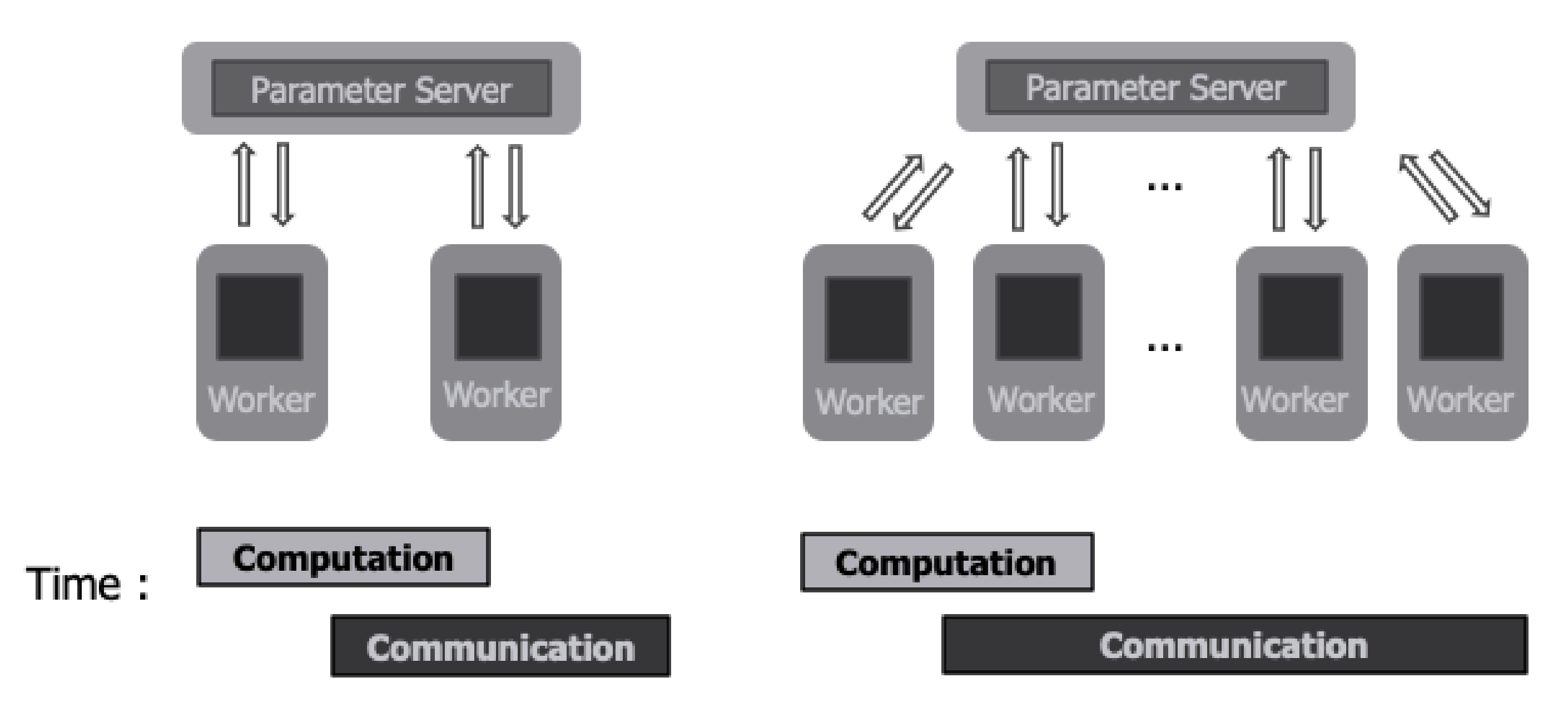Figure 1 shows a distributed deep learning environment. When communication time increases as the number of workers increases, the computing resources of workers cannot be used efficiently. Therefore, in the case of existing deep learning systems, as the number of workers increases, total system throughput decreases according to the increase in workers [12,13,14]. According to Li, Youjie et al., when training the representative deep learning models AlexNet, ResNet-152, and VGG-16 through distributed deep learning in a cluster of five machines in a 10 Gbit network environment, about 75% of the total execution time was communication time [15,16,17,18]. Therefore, by optimizing communication to reduce communication time, distributed deep learning can be performed efficiently. In deep learning systems, the gradients computed by workers are highly sparse. Therefore, gradients with small values have less effect on the model parameters [19]. Therefore, gradients with small values do not affect learning even if they are not sent to the parameter server or accumulated and sent to the parameter server later. By using the characteristics of deep learning, gradients with small values are not sent to the parameter server, thereby reducing the size of communication data sent from the worker to the parameter server. Furthermore, it is possible to reduce the size of communication data from the parameter server to the worker by not sending the model parameters that have not been updated to the worker.

In this paper, we propose a new communication optimization method that can effectively mitigate the performance degradation due to communication overheads without degrading the accuracy. Our main contributions are as follows:

• First, we propose a new layer dropping scheme to reduce communication data. In the case of large-scale deep learning models, the number of model parameters is large, so the number of gradients computed by workers is also large. Therefore, it is inefficient to compare the threshold value with the value of each gradient computed by the worker. Our proposed scheme efficiently compresses communication data by comparing the representative value of each hidden layer of the deep learning model and a threshold. We used the average of the absolute values of the gradients as the representative value of each hidden layer. The worker converts the hidden layer for which the representative value is less than the threshold value into a list type of size oneand sends it to the parameter server. Furthermore, the parameter server converts the hidden layers that have not been updated into a list of size one and sends them to the worker. Hidden layers that are not sent to the parameter server are accumulated in the worker’s local cache. When the accumulated value is greater than the threshold, the hidden layer stored in the worker’s local cache is sent to the parameter server to ensure training accuracy.
• Second, we propose an efficient method to pick a threshold value. The threshold is a value that can reduce the size of the gradients that the worker will send to the parameter server by a ratio R from the size of the total gradients. It takes much time to calculate a threshold by reflecting all the gradients. Therefore, in this paper, we compute the threshold by replacing the value of each gradient with the L1 norm of the gradients included in each hidden layer. Since the L1 norm is the sum of the absolute values of each element of the vector, the L1 norm of the gradients of each hidden layer shows the effect of the gradients on the model parameters. By using the L1 norm of each hidden layer, a large number of gradients to be used for threshold calculation can be reduced to the number of hidden layers in the deep learning model. The threshold can be fixed at the value calculated at the beginning of training or can be calculated again at specific cycles. In our experiments, we calculated a new threshold every 100 steps.

We implement a distributed deep learning system and the proposed optimization scheme using MPI and TensorFlow and show improvement in performance when performing distributed deep learning through experiments. When communication is optimized by applying the layer dropping scheme proposed in this paper, we confirm that the communication time decreased by about 95% and the total deep learning execution time by about 85% in a 1 Gbit network environment.

The rest of the paper is organized as follows. We present the related work in Section 2. In Section 3, we describe the architecture of distributed deep learning as a background. The layer dropping scheme we proposed is described in detail in Section 4. In addition, Section 5 describes how to compute a threshold value for performing layer dropping. In Section 6, we evaluate the performance of the proposed communication optimization scheme. Finally, we conclude our paper in Section 7.

2. Related Works

To accelerate distributed deep learning, INCEPTIONN (In-Network Computing to Exchange and Process Training Information Of Neural Networks) was proposed [15]. INCEPTIONN implements a communication data compression algorithm in hardware to accelerate distributed learning. When INCEPTIONN is applied, communication time is reduced by up to 80.7%, and deep learning is performed up to 3.1 times faster than existing distributed deep learning systems. Unlike INCEPTIONN, we implemented a communication optimization scheme in software to accelerate the distributed deep learning system.

In order to accelerate the distributed deep learning system, a hybrid aggregation method can be used [8]. The hybrid aggregation method uses a parameter server structure and an all-reduce structure together to optimize communication data. In the case of intra-node communication, local aggregation is performed by communicating in an all-reduce method. In the case of inter-node communication, a process called a local parameter server is executed for each node to communicate with the global parameter server. Therefore, the hybrid aggregation method can accelerate distributed deep learning by optimizing communication data through local aggregation. Communication can be additionally optimized by applying the communication optimization scheme proposed in this paper to the hybrid aggregation method.

Alham Fikri Aji and Kenneth Heafield proposed sparse communication [19]. They showed that dropping 99% of all gradients did not significantly affect the training accuracy. They showed a 49% speedup on MNIST and a 22% speedup on NMT. However, since the MNIST used in their experiments is a very simple deep learning model, it cannot be said to work correctly even on large models. Furthermore, in the case of gradient dropping, there is a disadvantage that overhead due to compression may increase because every gradient must be compared with the threshold.

AdaComp (Adaptive residual gradient Compression) is a gradient compression technique proposed for efficient communication in a distributed deep learning environment [20]. AdaComp divides each layer into bins to efficiently sample residues. It finds the largest absolute value of the residues in each bin. In AdaComp, the residue in each mini-batch is calculated as the sum of the previous residue and the latest gradient values obtained from back propagation. If the sum of the previous residue and the latest gradient multiplied by the scale-factor is greater than the maximum value of the bin, the residue is sent. AdaComp showed a maximum compression ratio of 200 times for fully-connected layers and recurrent layers. In addition, it showed a compression rate of up to 40 times for convolutional layers. Unlike AdaComp, we perform compression in units of layers of the deep learning model. Furthermore, in the case of AdaComp, there is a limitation in that the compression rate cannot be determined.

TernGrad is proposed to accelerate distributed deep learning in data parallelism [21]. TernGrad only uses three numeric levels {−1, 0, 1} for communication to reduce communication time. Furthermore, layer-wise ternarizing and gradient clipping to improve convergence are proposed. Ternarizing randomly quantizes the square of the gradients into a ternary vector of {−1, 0, +1}. Experiments showed that there is little or no loss of accuracy even when TernGrad is applied when performing distributed deep learning. TernGrad increased image throughput by 3.04 times when AlexNet [16] was trained using eight GPUs in a 1 Gbit Ethernet environment. When using 128 nodes in a high performance computing environment using Infiniband, using TernGrad doubled the training speed. Unlike TernGrad, our proposed scheme does not transform gradients computed by workers.

3. Distributed Deep Learning Architecture

Distributed deep learning using multiple GPUs/nodes can be used to solve the increasing training time of deep learning. The training method of distributed deep learning can be divided into two types—data parallelism and model parallelism. Data parallelism is a method of training the same deep learning model on multiple GPUs. In data parallelism, each worker trains a training model using different input data. As a result, the gradients calculated by each worker are different. Therefore, in order to update parameters when performing distributed deep learning through data parallelization, gradients calculated by each worker must be aggregated. Typical architectures that aggregate gradients are the parameter server architecture [11] and the all-reduce architecture [22]. 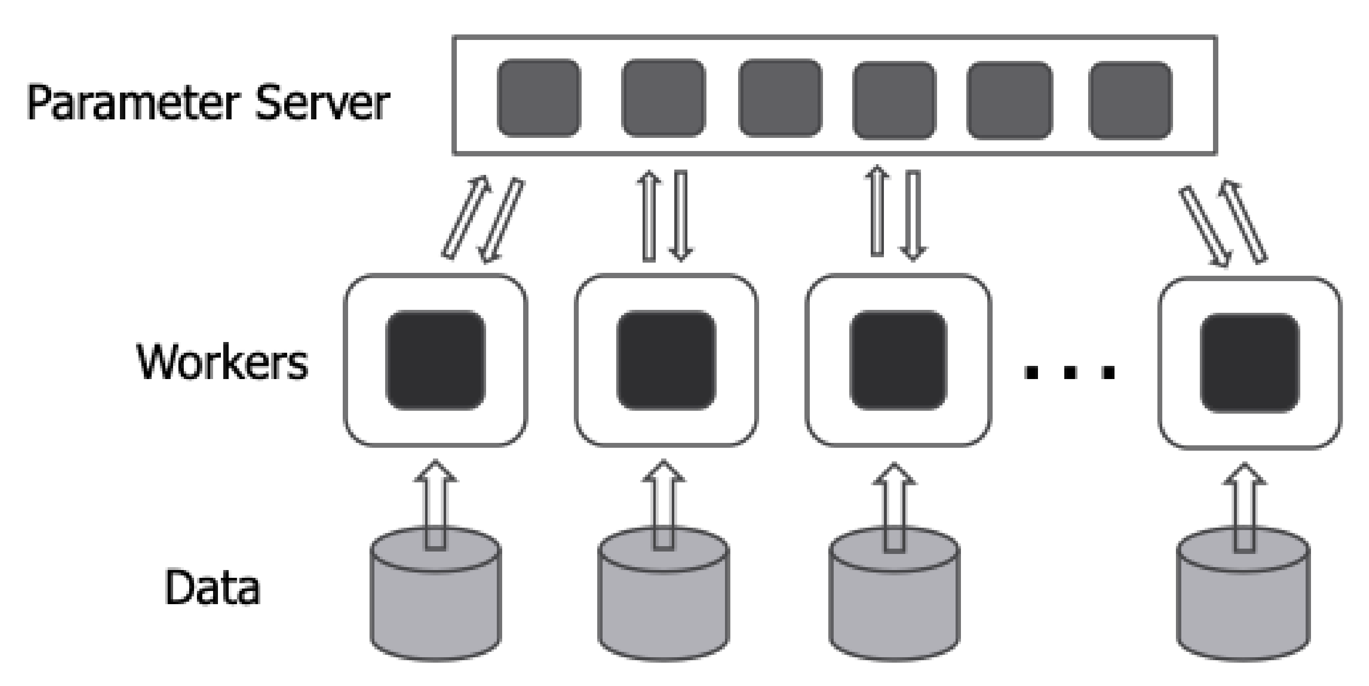Figure 2 depicts the parameter server architecture.

In the parameter server architecture, processes can be divided into two types—the parameter servers and workers. The parameter server receives gradients calculated from workers and updates the model parameters. Furthermore, the parameter server sends the latest model parameters that the parameter server has to the worker who needs them. Workers receive model parameters from the parameter server and compute gradients using input data and the deep learning model. The parameter server architecture can be performed synchronously or asynchronously. In a synchronous way, the parameter server updates model parameters after receiving gradients from all workers. After updating the model parameters, the parameter server sends the updated model parameters to all workers. Therefore, in the synchronous method, all workers perform training with the same model parameters. In an asynchronous way, the parameter server applies gradients to the model parameter whenever it receives gradients from a worker. Furthermore, the parameter server sends the model parameter immediately when there is a worker requesting the latest model parameter. Therefore, in the asynchronous method, each worker does not need to wait for other workers and trains with different model parameters. Distributed TensorFlow is a deep learning framework that supports the parameter server architecture [23]. In the case of the parameter server architecture, multiple workers communicate with one or a few parameter servers. Therefore, communication time increases as the number of workers increases, as shown in Figure 1. As the communication time increases, the entire computing resources of GPUs used for distributed deep learning cannot be efficiently used. Therefore, when using the parameter server architecture, communication needs to be optimized in order to efficiently utilize the computing resources of GPUs and increase scalability.

The all-reduce architecture aggregates gradients computed by each other through Peer-to-Peer (P-to-P) communication between workers without a central server. Therefore, unlike the parameter server architecture, there is no need to perform communication between the parameter server and the worker. As a result, communication overhead is reduced compared to the parameter server. However, the all-reduce architecture has the disadvantage that it can only operate synchronously. Uber’s Horovod is a representative distributed deep learning framework that operates with an all-reduce architecture [22].

4. Communication Optimization Schemes

In this paper, the bottleneck caused by communication is alleviated by compressing communication data in units of hidden layers when performing distributed deep learning. When performing deep learning, gradients with a small value among the gradients computed by the worker do not significantly affect the change of model parameters [19]. Therefore, we reduce communication data by not transmitting some hidden layers, which contain many gradients that do not affect the model parameters, to the parameter server. In order to distinguish between the hidden layer not to be transmitted and the hidden layer to be transmitted, we compare the representative value of each hidden layer and the threshold. The representative value of each hidden layer is the average of the absolute values of gradients included in the hidden layer.

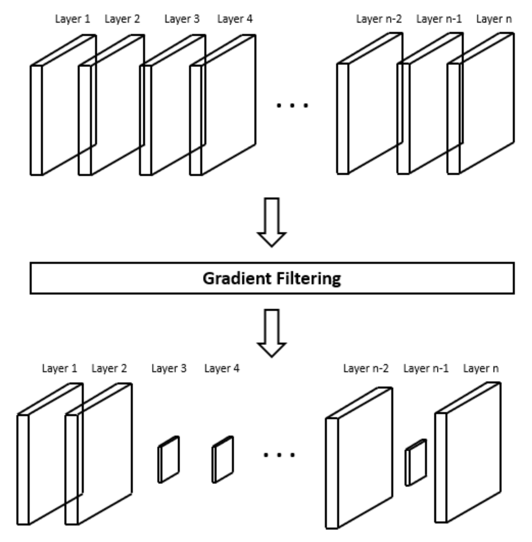
Figure 3 shows the change of communication data size through layer dropping. The top of Figure 3 is the original artificial neural network before layer dropping is applied. The bottom of Figure 3 is the compressed artificial neural network model after layer dropping is applied. As shown in Figure 3, when the layer dropping is applied, the size of the artificial neural network used for communication is reduced compared to the original artificial neural network. Therefore, when the compressed artificial neural network is transmitted, the communication time is reduced compared to when the original artificial neural network is transmitted.

4.1. Operation of the Worker for Communication Optimization

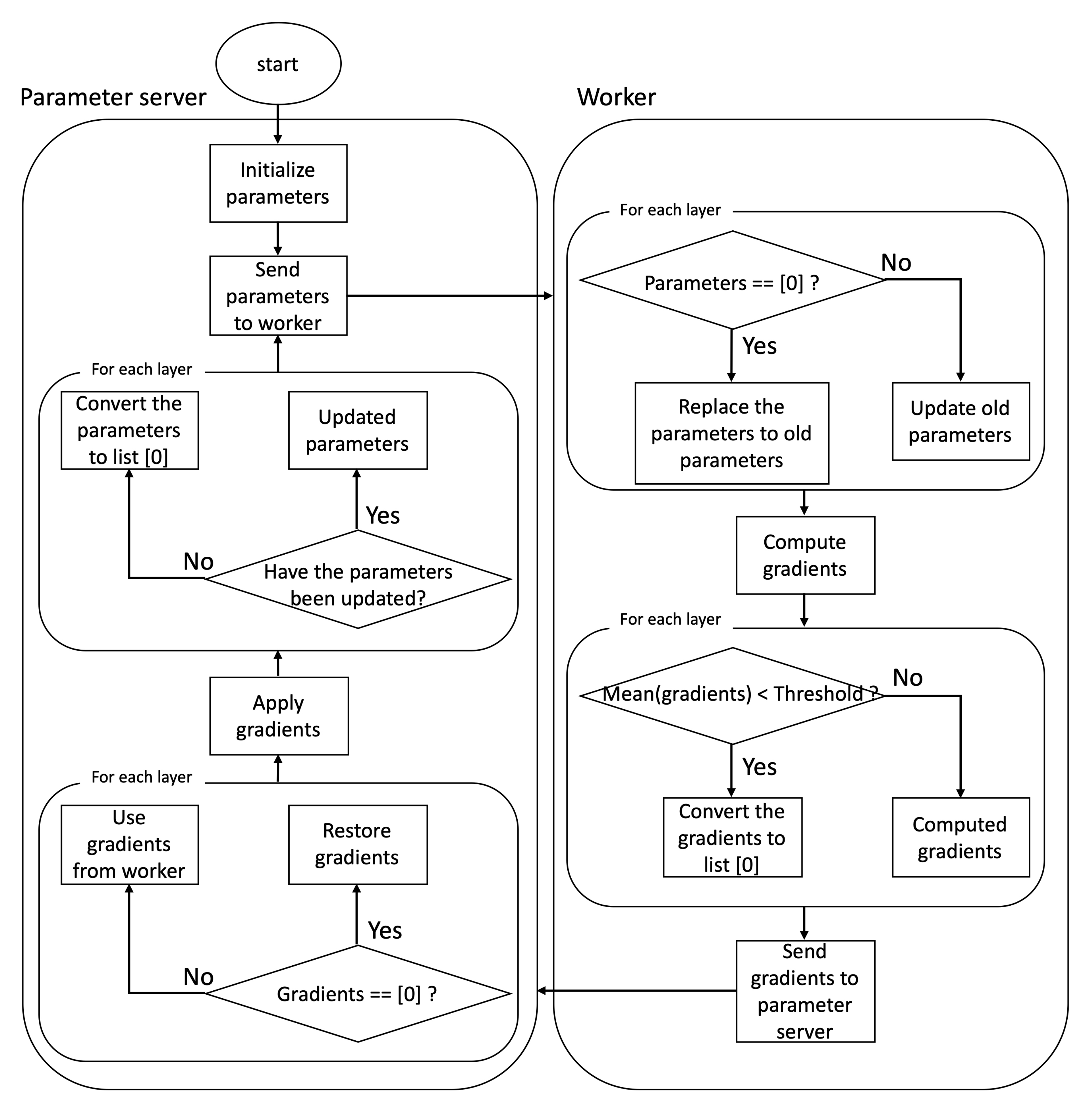
The right side of Figure 4 shows how the worker operates when performing distributed deep learning by applying layer dropping. When distributed deep learning is started, the worker receives initialized model parameters from the parameter server. The worker checks whether each layer of the received model parameter is a list [0]. The list [0] is a compressed hidden layer and a list with a size of one and a value of zero. In the first iteration, the worker receives the model parameters initialized by the parameter server, so all hidden layers are not the list [0]. However, after the first iteration, the worker receives compressed data from the parameter server. Therefore, some hidden layers may be the list [0]. Among the hidden layers of the received model parameter, the layers with [0] are replaced with the old parameters that the workers already had. In the case of a layer other than the list [0], the old parameters that the worker had are updated with the new parameters received from the parameter server. After that, the worker computes gradients using the updated parameters. After computing the gradients, the worker performs the following tasks to compress the data to be transmitted to the parameter server. The worker compares the predetermined threshold with the mean of the computed gradients on each layer. We will present how to pick the threshold value in the next section. If the mean of the gradients is less than the threshold, the layer is changed to a list [0]. If the average of gradients is larger than the threshold, the computed gradients are maintained. The worker compresses gradients based on the threshold and sends the compressed gradients to the parameter server.

4.2. Operation of the Parameter Server for Communication Optimization

The left side of Figure 4 shows how the parameter server operates when performing distributed deep learning by applying layer dropping. When training starts, the parameter server initializes the model parameters and sends them to workers. After the first step, the parameter server sends compressed model parameters to the workers. When the workers send compressed gradients calculated using the model parameters sent by the parameter server, the parameter server searches the list [0] among the received gradients. When the parameter server finds the list [0], the parameter server converts the list [0] to the shape of the original layer and fills the converted list with zeros using the shape information of the layer that the parameter server has. After restoring all the list [0] to the original shape, the parameter server updates the model parameters using the restored gradients. Before sending the updated parameter to the worker, the parameter server compresses the parameters to be sent. To compress the parameters, the parameter server checks whether each layer has been updated or not. The parameter server compresses the parameters to be transmitted by replacing the un-updated layer with the list [0]. The compressed parameters are sent to the workers.

4.3. Gradient Accumulation

Training accuracy may decrease due to layer dropping. The loss of training accuracy can be avoided by applying gradient accumulation [24]. Therefore, to avoid the loss of training accuracy, we perform layer accumulation. Gradient accumulation is performed in each worker. To perform layer accumulation, gradients of the hidden layer that are not sent to the parameter server are stored and accumulated in the local cache of each worker. When the average of the accumulated hidden layer gradients stored in each worker’s local cache exceeds the threshold, the gradients stored in the local cache are sent to the parameter server. The specific layer compression and accumulation method is as follows. When there are N gradients of the hidden layer in the tth iteration, the ith gradient is $gradients{\left(t\right)}_i$, and the ith of the N accumulated gradients of the hidden layer is $accum{\left(t\right)}_i$.

$$accum{\left(t\right)}_i=accum{(t-1)}_i+gradients{\left(t\right)}_i$$

(1)

$$\frac{{\sum }_{i=1}^{N}accum{\left(t\right)}_i}{N}<Threshold$$

(2)

The initial value of $accum{\left(0\right)}_i$ is zero, and the gradients computed by each worker are added to the gradients stored in each worker’s local cache for each iteration. After that, the average of the gradients of each hidden layer is calculated. Hidden layers whose average gradients are smaller than the threshold are stored in the worker’s local cache again.

5. How to Calculate the Threshold

The threshold used in this paper is a value that can drop the number of gradients transmitted to the parameter server close to a predetermined ratio R. It takes a very long time to calculate the threshold by reflecting all the gradients. Therefore, in this paper, the value of each gradient is replaced with the L1 norm of the gradients included in each hidden layer. This replaces very large amounts of gradients with very small amounts. The same effect can be achieved by using the L2 norm instead of the L1 norm. The L1 norm is the sum of the absolute values of each element of the vector. In the case of the L2 norm, it represents the magnitude of a vector in n-dimensional space, so it can be obtained as the square root of the sum of the squares of each element. Therefore, we use the L1 norm, which is relatively easy to compute. Using the obtained L1 norm of each hidden layer and the size of the hidden layer, we calculate the L1 norm value of the layer that enables the transmission of gradients as much as $(1-R)\ast \left(totalnumberofgradients\right)$, and this value is designated as the threshold value. When R becomes larger, a lesser amount of communication data is transferred between each worker and the parameter server. Therefore, as R is increased, communication time can be reduced, but training accuracy can be decreased due to an increase in the amount of gradients to be dropped. The threshold is computed on each worker. Since the threshold value is necessary to compress the gradients, they are stored only in each worker, and the parameter server does not store the threshold information of workers. The calculated threshold value can be used by fixing the value obtained at the beginning of training, or it can be newly calculated at a certain step according to the DNN (Deep Neural Network) model, the type and number of data sets, and the decay setting of the learning rate. In our experiments, a new threshold is calculated every 100 iterations.

Algorithm 1 is the pseudocode of the algorithm to find the threshold. First, the threshold is initialized to −1. After that, inverse sorting is performed based on the representative value of each hidden layer. The representative value of each hidden layer we used is the L1 norm of the hidden layer. The L1 norm is the sum of the absolute values of the elements of the vector. Therefore, it is possible to express the parameter change due to the gradients included in each layer. When the hidden layer is aligned, the number of gradients to be dropped is initialized to zero. After that, the number of gradients contained in the ith hidden layer is accumulated and stored in the number of gradients to be dropped. When the number of gradients to be dropped is greater than the $totalnumberofgradients\ast R$, the iteration stops. The threshold is the representative value of the last added hidden layer. If the threshold is not found even though it is repeated as many times as the number of hidden layers, the threshold is −1. Therefore, if the threshold is −1, it means an invalid threshold.

Algorithm 1 Threshold searching algorithm.

6. Evaluations

We conducted experiments in two environments to demonstrate the performance of the proposed communication optimization scheme. In the first experiment, a network is constructed with 1 Gbit Ethernet to evaluate the performance of the communication optimization scheme in a low bandwidth network environment. In the second experiment, a network is constructed with 56 Gbit Ethernet to evaluate the performance of the communication optimization scheme in a high performance computing environment.

6.1. Performance of Layer Dropping in a 1 Gbit Network Environment

The first experiment was conducted in an environment consisting of one parameter server machine and two worker machines. Each worker machine consisted of two NVIDIA Geforce GTX 1080 Tis. The parameter server uses the CPU to update and maintain model parameters. Each worker uses the GPU to compute gradients and send computed gradients to the parameter server. The network is composed of 1 Gbit Ethernet. We used ResNet v1 50 as a training model. Furthermore, we implemented a distributed environment using OpenMPI 3.0.0 and TensorFlow 1.13.

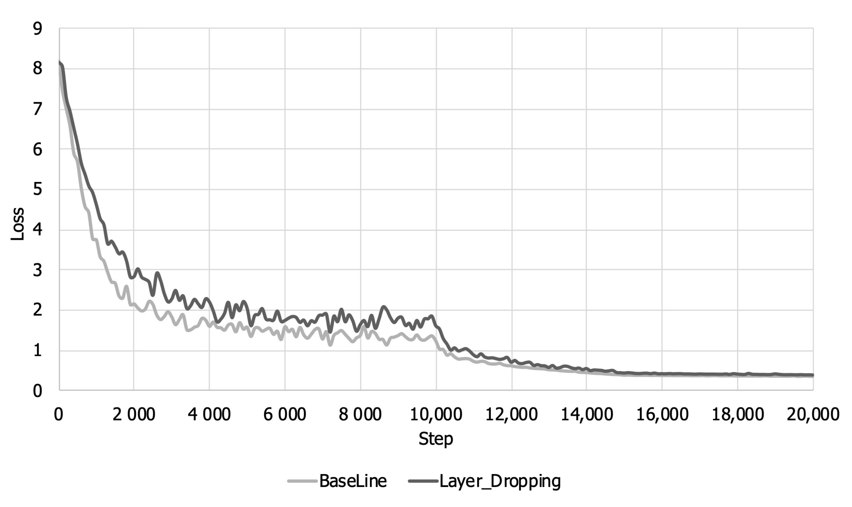
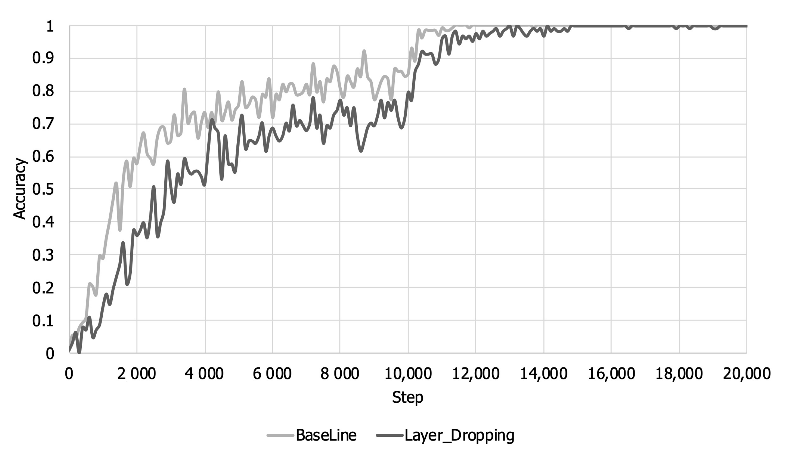
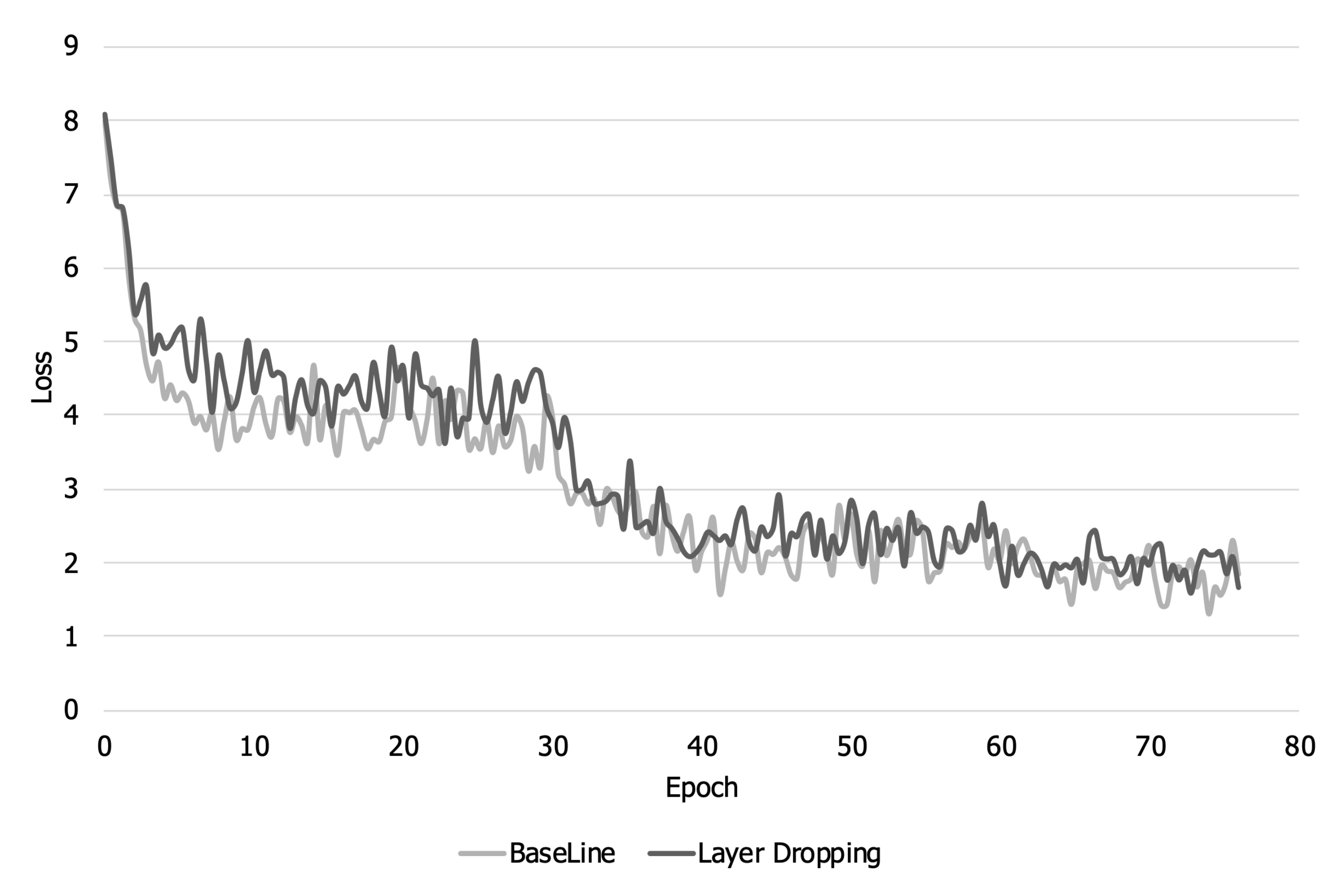
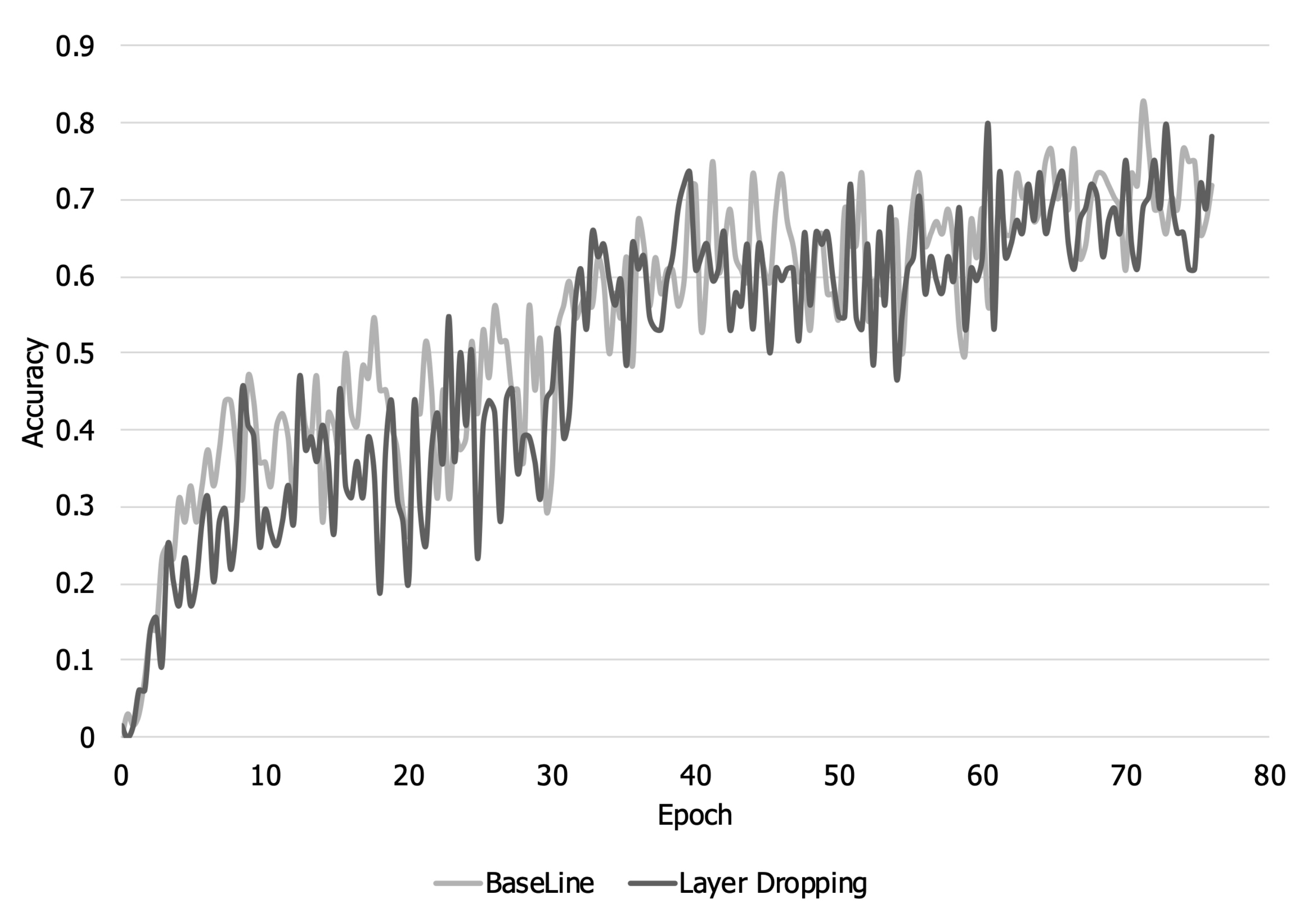
Figure 5 and Figure 6 show the training accuracy and loss over the training steps. As shown in Figure 5, when layer dropping is applied, the training loss is larger than that when layer dropping is not applied until about 14,000 steps because training about some layers whose representative value is less than the threshold is not reflected in the early part of the training. Looking at Figure 6, it can be seen that there is a loss of accuracy due to layer dropping before about 14,000 steps. The training accuracy decreases for the same reason that loss increases. However, layers that were not reflected in the model parameter at the beginning of learning are reflected later due to gradient accumulation. Therefore, even when layer dropping is applied, the training loss and accuracy eventually converge equally with the baseline.

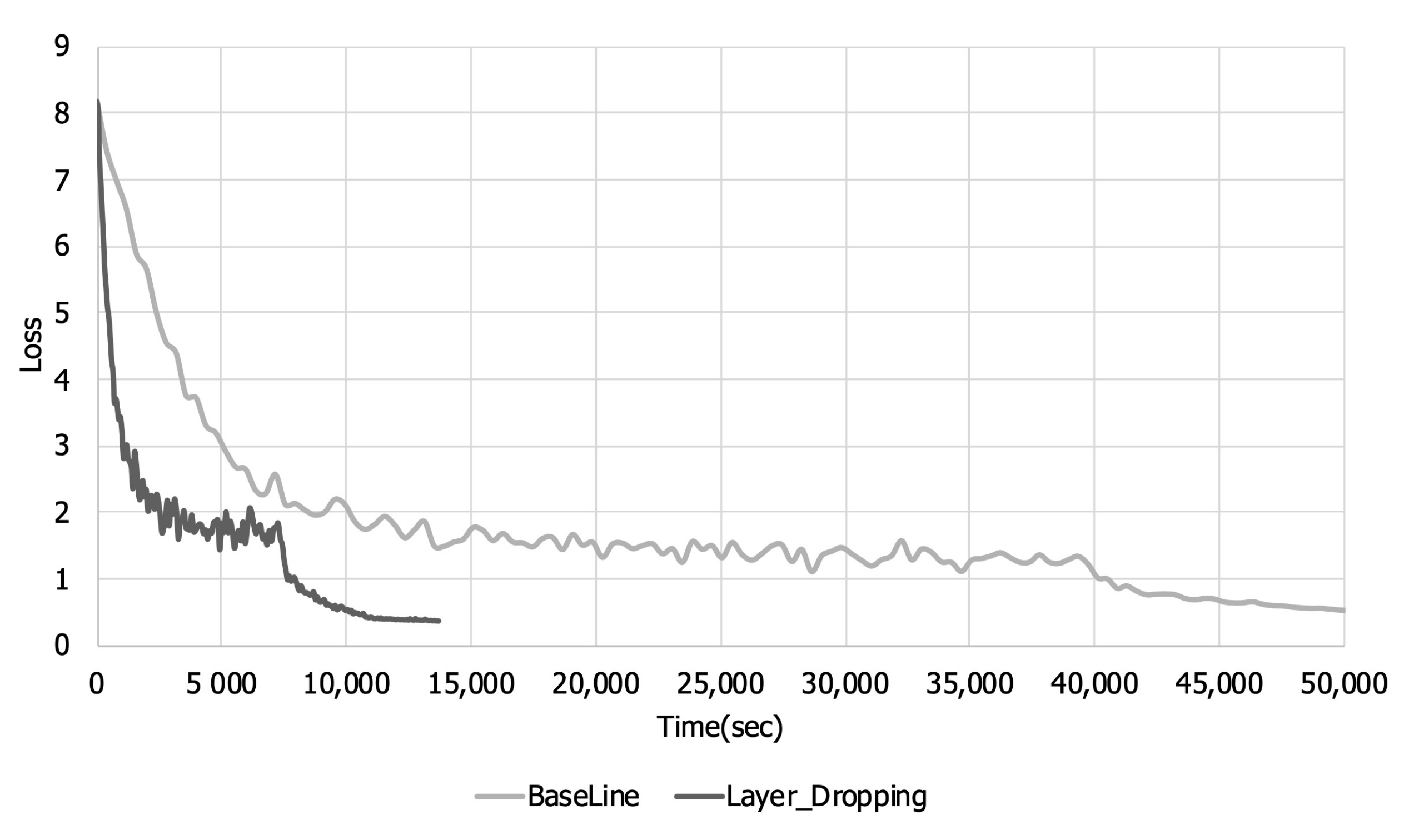
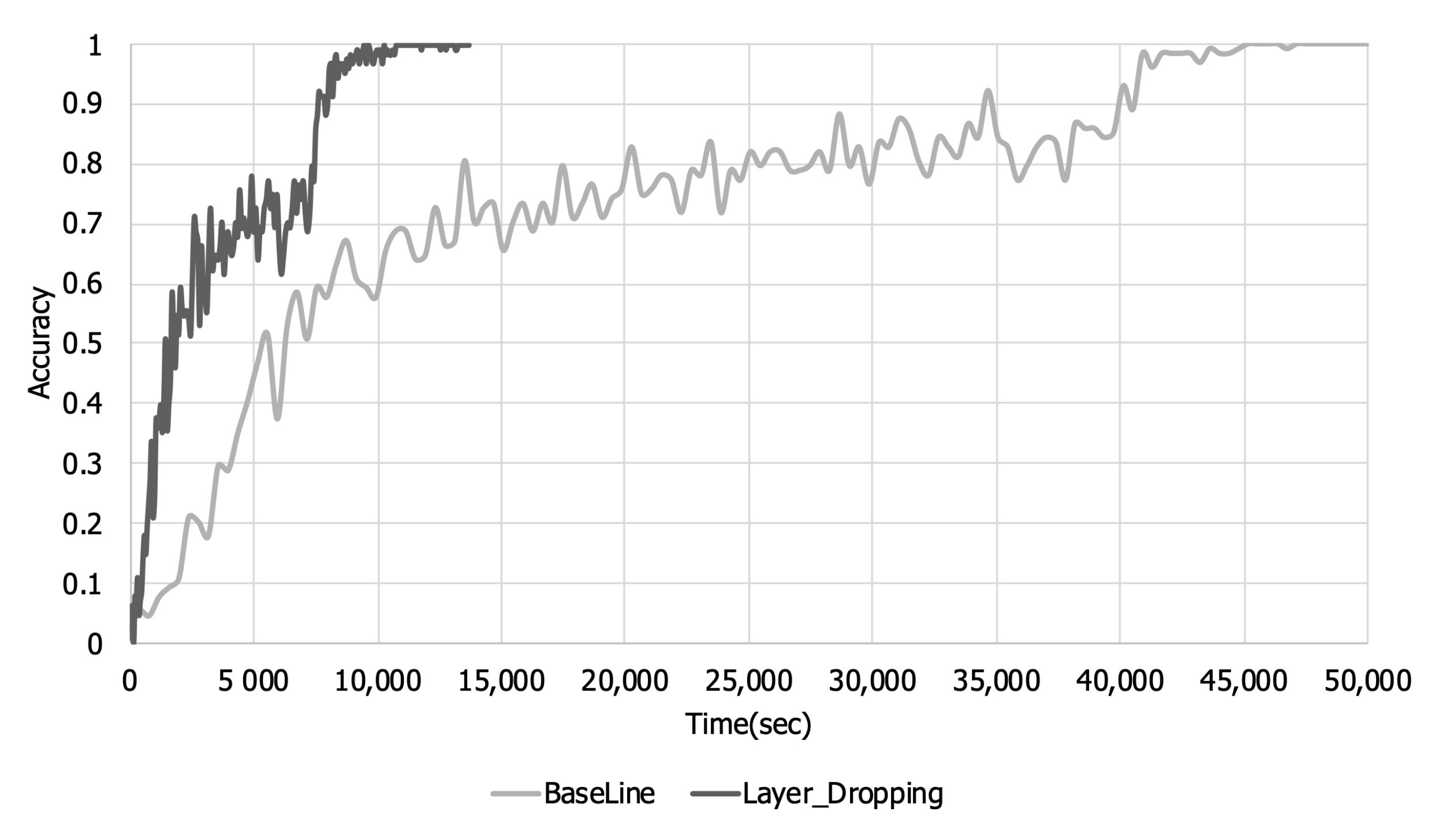
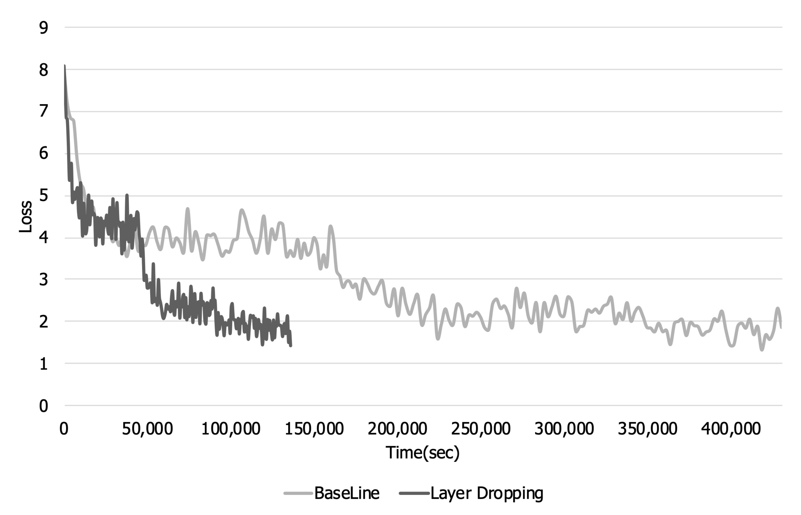
Figure 7 and Figure 8 are graphs of the training loss and accuracy over the training time. Looking at Figure 5 and Figure 6, it can be seen that there is a loss in training accuracy and a loss per step due to layer dropping. However, when layer dropping is applied, the time required to learn one step is reduced due to the reduction in communication time. Looking at Figure 7 and Figure 8, when layer dropping was applied, the loss and training accuracy converged in about 14,000 s. On the other hand, in the case of the original, it took about 50,000 s for the loss and training accuracy to converge. These results show that when layer dropping is applied, distributed learning can be performed more quickly by performing communication efficiently.

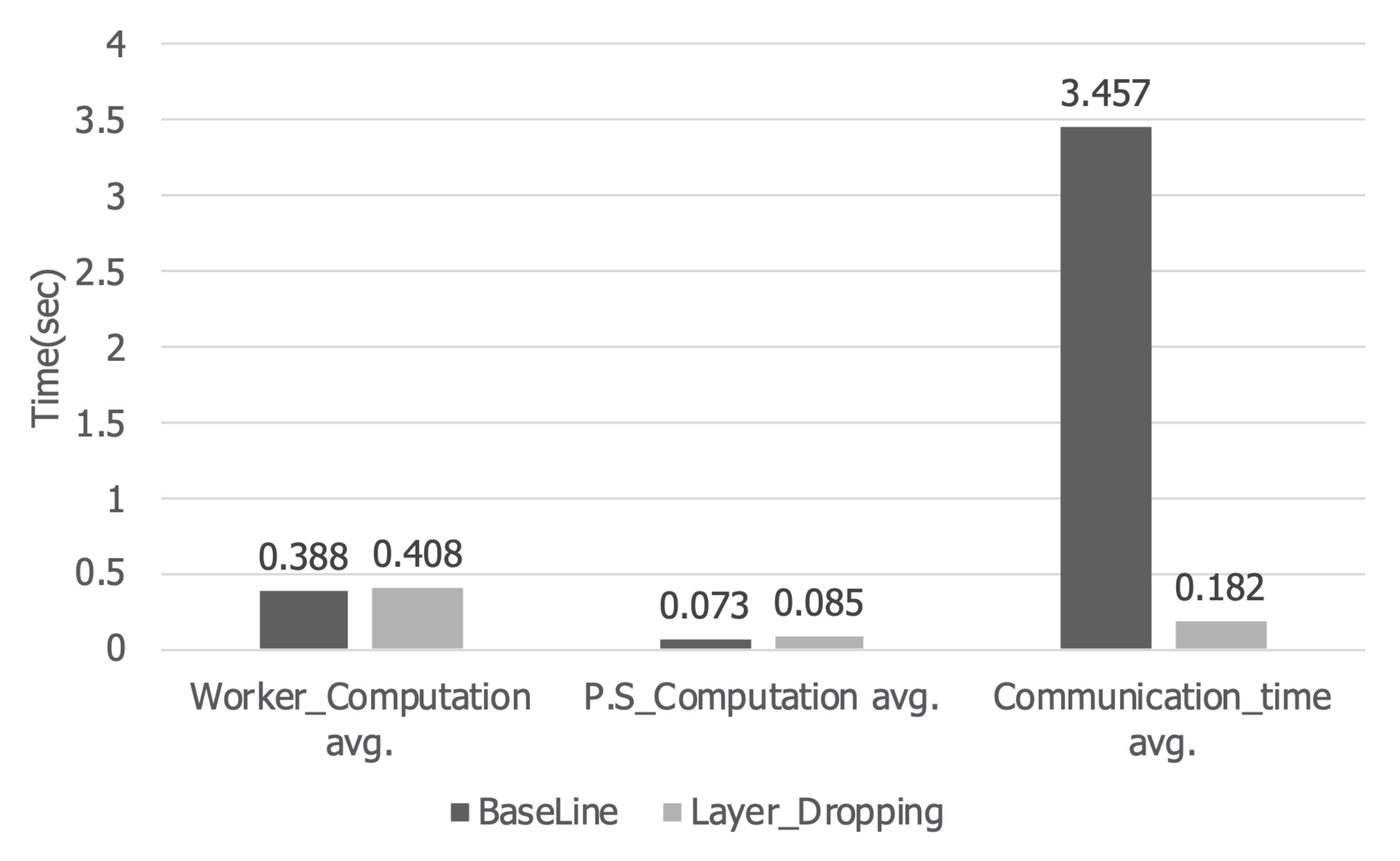
Figure 9 shows the computation time and communication time of the worker and parameter server per iteration. When layer dropping was applied, the computation time of the worker increased by about 5% from 0.388 s to 0.408 s. In addition, the computation time of the parameter server increased by about 15% from 0.073 s to 0.085 s. However, in the case of communication time, it decreased about 95% from 3.457 s to 0.182 s. Therefore, the total execution time was reduced by about 82%, so that training can be performed faster than the existing distributed deep learning.

6.2. Performance of Layer Dropping in a 56 Gbit Network Environment

The second experiment was carried out using four machines. One of the four machines had a parameter server and two workers running, and the other three machines had two workers each. The second experiment was performed using KISTI’s (Korea Institute of Science and Technology Information) Neuron [25]. Each machine consisted of an Intel Xeon Skylake and two NVIDIA Tesla V100s. The network was configured with 56 Gbit Ethernet. As a training model, the ResNet v1 50 model was used. ImageNet was used as the data set for training the model. Furthermore, like the previous experiment, a distributed deep learning environment was implemented using OpenMPI 3.0.0 and TensorFlow 1.13.1.

Figure 10 and Figure 11 show the loss per epoch and training accuracy. In Figure 10, when layer dropping is applied, the overall training loss is higher than the baseline. In addition, looking at Figure 11, it can be seen that the overall training accuracy decreases when layer dropping is applied.

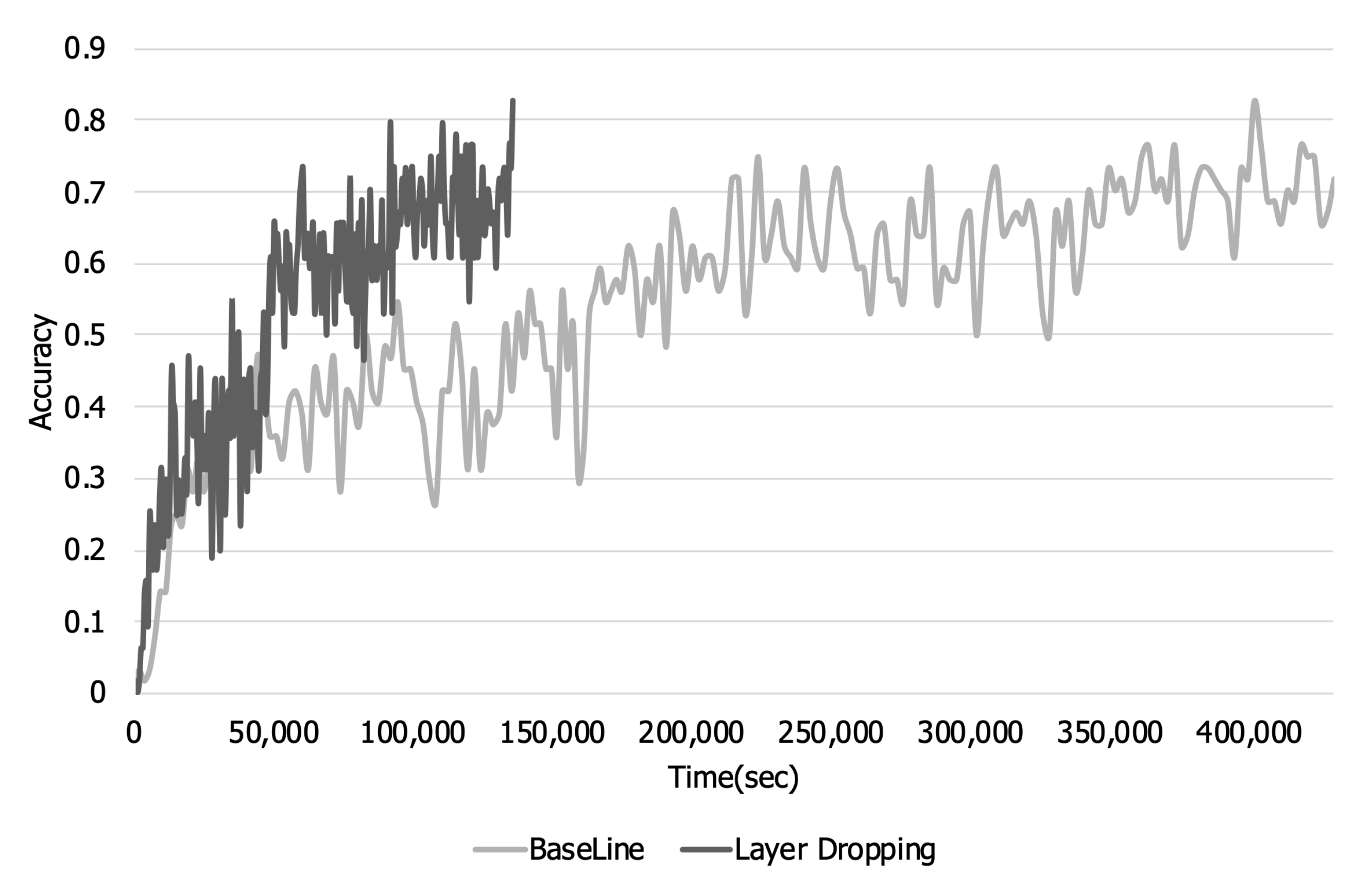
Figure 12 and Figure 13 show the training loss and accuracy over time. We conducted experiments until the accuracy in the case of applying layer dropping became similar to the baseline. In Figure 11, it can be seen that there is a loss in training accuracy due to layer dropping. However, even in a 56 Gbit Ethernet environment, the time required to perform each iteration decreases due to the decrease in communication time. Therefore, as shown in Figure 12, when layer dropping is applied, the training loss decreases faster than the baseline. Furthermore, Figure 13 shows that the training accuracy when layer dropping is applied increases faster than the baseline.

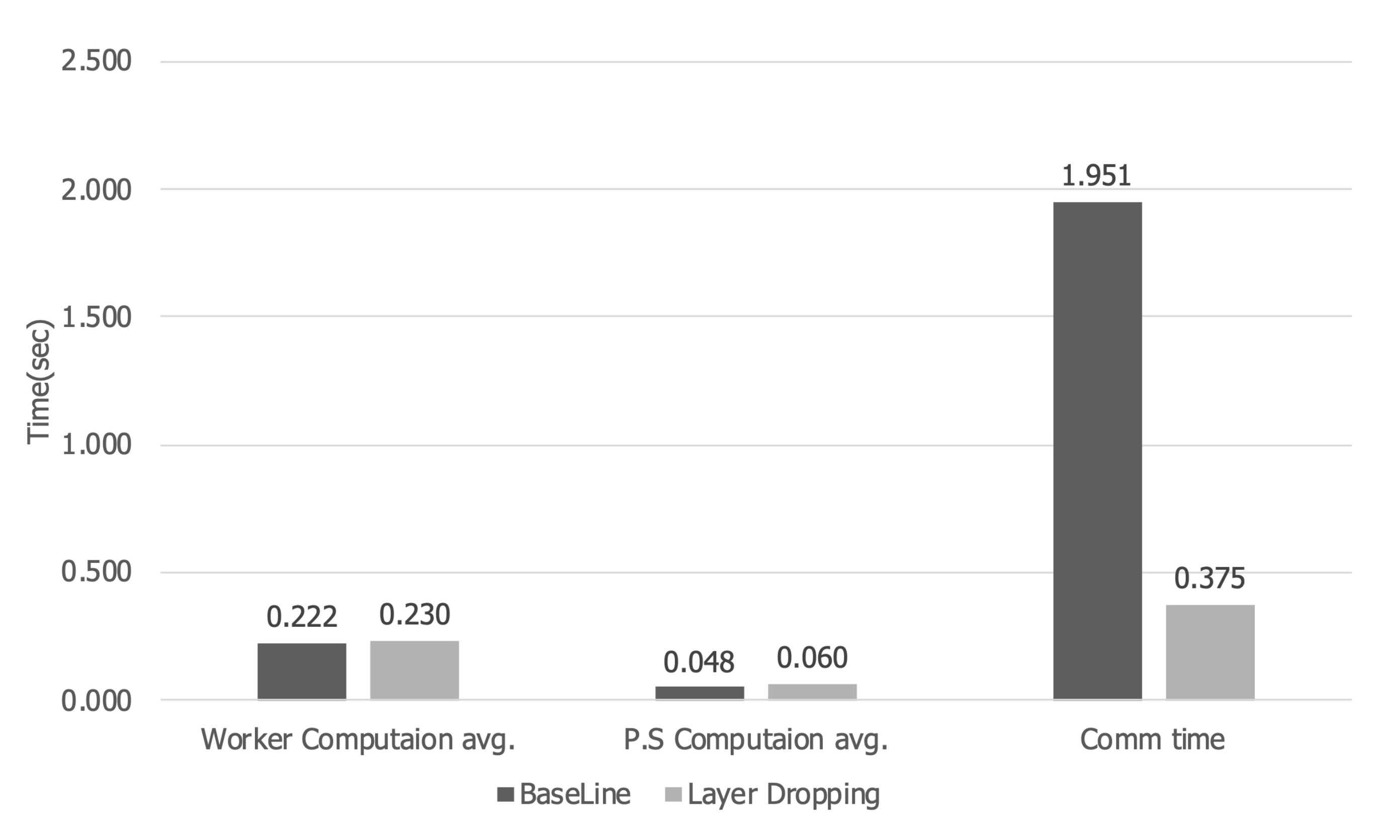
Figure 14 is a graph showing the computation time and communication time per iteration. When layer dropping is applied, the training time of the worker increases by 3.6% from 0.222 s to 0.230 s. Furthermore, the computation time of the parameter server increases by 23% from 0.048 s to 0.06 s. However, in the case of communication time, an 80.8% decrease from 1.951 s to 0.375 s can be seen. Therefore, the time to perform one iteration is reduced by about 70%, so that learning can be performed faster than the existing distributed learning.

6.3. Summary of the Experimental Results

Table 1. Average execution time per iteration.

Network	Layer Dropping	Worker Compute (sec)	Parameter Server Compute (sec)	Communication (sec)	Total (sec)
1 Gb/s	No	0.388	0.073	3.457	3.918
	Yes	0.408	0.085	0.182	0.675
56 Gb/s	No	0.222	0.048	1.951	2.222
	Yes	0.230	0.060	0.375	0.665

shows the average execution time per iteration when deep learning is performed. As shown in the table, when layer dropping is applied, the computation time of worker and parameter server increases. We performed compression on a layer basis to minimize overhead due to communication data compression. Therefore, the worker’s computation time increased by only about 5% in a 56 Gbit network environment. In the case of the parameter server, the computation time increased by up to about 23% in a 56 Gbit network environment. However, in a distributed deep learning system, the computational time of the parameter server took up very little. In our experiment, the computation time of the parameter server only increased by about 0.01 s. When layer dropping was applied, the computation time slightly increased, but the communication time decreased significantly. When layer dropping was applied, communication time was reduced by about 95% in a 1 Gbit Ethernet environment. As a result, the overall execution time was reduced by about 82%. In addition, even in a 56 Gbit Ethernet environment, which is a high bandwidth network, when layer dropping was applied, communication time was reduced by about 81% and total execution time by about 70%. Therefore, when the communication optimization scheme proposed in this paper is applied, communication can be efficiently performed not only in a low bandwidth network environment, but also in a high bandwidth network environment.

7. Conclusions

In this paper, we propose a communication optimization scheme for accelerating distributed deep learning systems. We perform compression in units of layers of the deep learning model. Therefore, our proposed compression scheme can perform compression more efficiently than comparing all gradients with a threshold. Furthermore, to reduce the overhead of calculating the threshold, we use the L1 norm of each hidden layer rather than using gradients when calculating the threshold. We implement a distributed deep learning environment using TensorFlow and MPI. To verify the performance of the proposed scheme according to the network performance, experiments are performed in both a 1 Gbit Ethernet environment and a 56 Gbit environment. We show through experiments that our compression method works efficiently not only in a low bandwidth network, but also in a high bandwidth network. In the future, we will conduct experiments by applying it to various large-scale deep learning models and optimizers.

References

- Deng, J.; Dong, W.; Socher, R.; Li, L.; Li, K.; Li, F.-F. ImageNet: A large-scale hierarchical image database. In Proceedings of the 2009 IEEE Conference on Computer Vision and Pattern Recognition, Miami, FL, USA, 20–25 June 2009; pp. 248–255. [Google Scholar]
- Szegedy, C.; Liu, W.; Jia, Y.; Sermanet, P.; Reed, S.; Anguelov, D.; Erhan, D.; Vanhoucke, V.; Rabinovich, A. Going deeper with convolutions. In Proceedings of the 2015 IEEE Conference on Computer Vision and Pattern Recognition (CVPR), Boston, MA, USA, 7–12 June 2015; pp. 1–9. [Google Scholar]
- Real, E.; Aggarwal, A.; Huang, Y.; Le, Q. Regularized Evolution for Image Classifier Architecture Search. arXiv 2018, arXiv:1802.01548. [Google Scholar] [CrossRef]
- Huang, Y.; Cheng, Y.; Bapna, A.; Firat, O.; Chen, D.; Chen, M.; Lee, H.; Ngiam, J.; Le, Q.V.; Wu, Y.; et al. Gpipe: Efficient training of giant neural networks using pipeline parallelism. In Proceedings of the Advances in Neural Information Processing Systems, Vancouver, BC, Canada, 8–14 December 2019; pp. 103–112. [Google Scholar]
- Zinkevich, M.; Weimer, M.; Li, L.; Smola, A.J. Parallelized Stochastic Gradient Descent. In Proceedings of the Advances in Neural Information Processing Systems 23, Vancouver, BC, Canada, 6–11 December 2010; pp. 2595–2603. [Google Scholar]
- Kim, Y.; Choi, H.; Lee, J.; Kim, J.; Jei, H.; Roh, H. Efficient Large-Scale Deep Learning Framework for Heterogeneous Multi-GPU Cluster. In Proceedings of the 2019 IEEE 4th International Workshops on Foundations and Applications of Self* Systems (FAS*W), Umea, Sweden, 16–20 June 2019; pp. 176–181. [Google Scholar]
- Kim, Y.; Lee, J.; Kim, J.; Jei, H.; Roh, H. Efficient Multi-GPU Memory Management for Deep Learning Acceleration. In Proceedings of the 2018 IEEE 3rd International Workshops on Foundations and Applications of Self* Systems (FAS*W), Trento, Italy, 3–7 September 2018; pp. 37–43. [Google Scholar]
- Kim, Y.; Choi, H.; Lee, J.; Kim, J.S.; Jei, H.; Roh, H. Towards an optimized distributed deep learning framework for a heterogeneous multi-GPU cluster. Clust. Comput. 2020, 23. [Google Scholar] [CrossRef]
- Kim, Y.; Lee, J.; Kim, J.S.; Jei, H.; Roh, H. Comprehensive techniques of multi-GPU memory optimization for deep learning acceleration. Clust. Comput. 2020, 23, 2193–2204. [Google Scholar] [CrossRef]
- Naumov, M.; Kim, J.; Mudigere, D.; Sridharan, S.; Wang, X.; Zhao, W.; Yilmaz, S.; Kim, C.; Yuen, H.; Ozdal, M.; et al. Deep Learning Training in Facebook Data Centers: Design of Scale-up and Scale-out Systems. arXiv 2020, arXiv:2003.09518. [Google Scholar]
- Heigold, G.; McDermott, E.; Vanhoucke, V.; Senior, A.; Bacchiani, M. Asynchronous stochastic optimization for sequence training of deep neural networks. In Proceedings of the 2014 IEEE International Conference on Acoustics, Speech and Signal Processing (ICASSP), Florence, Italy, 4–9 May 2014. [Google Scholar]
- Zhang, H.; Zheng, Z.; Xu, S.; Dai, W.; Ho, Q.; Liang, X.; Hu, Z.; Wei, J.; Xie, P.; Xing, E.P. Poseidon: An efficient communication architecture for distributed deep learning on {GPU} clusters. In Proceedings of the 2017 {USENIX} Annual Technical Conference ({USENIX}{ATC} 17), Santa Clara, CA, USA, 12–14 July 2017; pp. 181–193. [Google Scholar]
- Sattler, F.; Wiedemann, S.; Müller, K.; Samek, W. Sparse Binary Compression: Towards Distributed Deep Learning with minimal Communication. In Proceedings of the 2019 International Joint Conference on Neural Networks (IJCNN), Budapest, Hungary, 14–19 July 2019; pp. 1–8. [Google Scholar] [CrossRef]
- Dong, J.; Cao, Z.; Zhang, T.; Ye, J.; Wang, S.; Feng, F.; Zhao, L.; Liu, X.; Song, L.; Peng, L.; et al. EFLOPS: Algorithm and System Co-Design for a High Performance Distributed Training Platform. In Proceedings of the 2020 IEEE International Symposium on High Performance Computer Architecture (HPCA), San Diego, CA, USA, 22–26 February 2020; pp. 610–622. [Google Scholar] [CrossRef]
- Li, Y.; Park, J.; Alian, M.; Yuan, Y.; Qu, Z.; Pan, P.; Wang, R.; Schwing, A.; Esmaeilzadeh, H.; Kim, N.S. A Network-Centric Hardware/Algorithm Co-Design to Accelerate Distributed Training of Deep Neural Networks. In Proceedings of the 2018 51st Annual IEEE/ACM International Symposium on Microarchitecture (MICRO), Fukuoka, Japan, 20–24 October 2018; pp. 175–188. [Google Scholar]
- Krizhevsky, A.; Sutskever, I.; Hinton, G.E. Imagenet classification with deep convolutional neural networks. Commun. ACM 2017, 60, 84–90. [Google Scholar] [CrossRef]
- He, K.; Zhang, X.; Ren, S.; Sun, J. Deep Residual Learning for Image Recognition. In Proceedings of the 2016 IEEE Conference on Computer Vision and Pattern Recognition (CVPR), Las Vegas, NV, USA, 27–30 June 2016; pp. 770–778. [Google Scholar] [CrossRef]
- Simonyan, K.; Zisserman, A. Very Deep Convolutional Networks for Large-Scale Image Recognition. In Proceedings of the 3rd International Conference on Learning Representations, ICLR 2015, San Diego, CA, USA, 7–9 May 2015. [Google Scholar]
- Aji, A.F.; Heafield, K. Sparse Communication for Distributed Gradient Descent. In Proceedings of the 2017 Conference on Empirical Methods in Natural Language Processing, Copenhagen, Denmark, 7–11 September 2017; Association for Computational Linguistics: Copenhagen, Denmark, 2017; pp. 440–445. [Google Scholar] [CrossRef]
- Chen, C.; Choi, J.; Brand, D.; Agrawal, A.; Zhang, W.; Gopalakrishnan, K. AdaComp: Adaptive Residual Gradient Compression for Data-Parallel Distributed Training. In Proceedings of the Thirty-Second AAAI Conference on Artificial Intelligence, (AAAI-18), The 30th Innovative Applications of Artificial Intelligence (IAAI-18), and The 8th AAAI Symposium on Educational Advances in Artificial Intelligence (EAAI-18), New Orleans, LA, USA, 2–7 February 2018; McIlraith, S.A., Weinberger, K.Q., Eds.; AAAI Press: Palo Alto, CA, USA, 2018; pp. 2827–2835. [Google Scholar]
- Wen, W.; Xu, C.; Yan, F.; Wu, C.; Wang, Y.; Chen, Y.; Li, H. TernGrad: Ternary Gradients to Reduce Communication in Distributed Deep Learning. In Proceedings of the 31st International Conference on Neural Information Processing Systems—NIPS’17, Long Beach, CA, USA, 4–9 December 2017; Curran Associates Inc.: Red Hook, NY, USA, 2017; pp. 1508–1518. [Google Scholar]
- Sergeev, A.; Balso, M.D. Horovod: Fast and easy distributed deep learning in TensorFlow. arXiv 2018, arXiv:1802.05799. [Google Scholar]
- TensorFlow: An Open Source Machine Learning Library for Research and Production. Available online: https://www.tensorflow.org/ (accessed on 10 November 2020).
- Lin, Y.; Han, S.; Mao, H.; Wang, Y.; Dally, W.J. Deep gradient compression: Reducing the communication bandwidth for distributed training. arXiv 2017, arXiv:1712.01887. [Google Scholar]
- KISTI Neuron. Available online: https://www.ksc.re.kr/eng/resource/neuron (accessed on 10 November 2020).