Article

A Deep-Learning-Based Bearing Fault Diagnosis Using Defect Signature Wavelet Image Visualization

1
School of Electrical, Electronics and Computer Engineering, University of Ulsan, Ulsan 44610, Korea
2
ICT Convergence Safety Research Center, University of Ulsan, Ulsan 44610, Korea
3
School of Computer Science and Engineering, Soongsil University, Seoul 06978, Korea
*
Author to whom correspondence should be addressed.
Appl. Sci. 2020, 10(24), 8800; https://doi.org/10.3390/app10248800
Submission received: 5 November 2020 / Revised: 6 December 2020 / Accepted: 8 December 2020 / Published: 9 December 2020
(This article belongs to the Special Issue Machine Fault Diagnostics and Prognostics II)

Abstract

:
A new method is established to construct the 2-D fault diagnosis representation of multiple bearing defects from 1-D acoustic emission signals. This technique starts by applying envelope analysis to extract the envelope signal. A novel strategy is propounded for the deployment of the continuous wavelet transform with damage frequency band information to generate the defect signature wavelet image (DSWI), which describes the acoustic emission signal in time-frequency-domain, reduces the nonstationary effect in the signal, shows discriminate pattern visualization for different types of faults, and associates with the defect signature of bearing faults. Using the resultant DSWI, the deep convolution neural network (DCNN) architecture is designed to identify the fault in the bearing. To evaluate the proposed algorithm, the performance of this technique is scrutinized by a series of experimental tests acquired from a self-designed testbed and corresponding to different bearing conditions. The performance from the experimental dataset demonstrates that the suggested methodology outperforms conventional approaches in terms of classification accuracy. The result of combining the DCNN with DSWI input yields an accuracy of 98.79% for classifying multiple bearing defects.

1. Introduction

Indisputably, rotary machinery is broadly utilized across production industries such as in power systems, petrochemicals and means of transportation due to its low cost, rugged high efficiency under a heavy load, reliability, and robust design. Generally, the consequence of rotary machinery obliged to operate for prolonged periods under harsh-condition environments is wear and tear, which is associated with mechanical stresses, which can lead to unexpected failure in bearings and gears, which are crucial components in a rotary machine. Such failures could lead to economic losses or human casualties. As a consequence, the machine’s health supervision and fault analysis are vital integral elements of the maintenance procedure in industrial manufacturing. A robustly conditioned monitoring procedure can improve productivity, reduce maintenance expenses, and enhance reliability and safety.
While gear and bearing faults commonly betide the rotary machine, bearing faults prevail in occurrence. Industrial statistics illustrate that 40% of total large machine breakdowns happened due to broken bearings while for small machines, the analogous number reaches up to 90% [1]. Therefore, real-time monitoring and fault diagnosis methods for rolling element bearings have accrued considerable attention from researchers in recent years. Normally, there are three primary categories for fault diagnosis methods including reactive, preventive, and predictive maintenance [2]. Fault diagnosis methods can also be categorized as data-driven-based (knowledge-based), model-based, and hybrid-based with the hybrid-based method considered as the combination of one or several methods of model-based and data-driven-based [3,4,5]. In model-based fault diagnosis, the bearing system is analyzed by constructing an equivalent mathematical model that describes the differences between the normal state and fault states; however, the model-based method can be complicated by the increasing non-linearity of the system. The computational cost increases when the complexity of the system increases [6,7]. Data-driven-based methods are based on measurements taken over time and with data analysis to yield an assessment about the physical state of the machine [8,9]. With the developments in acquisition devices and sensors, communication technology, availability of data such as big data and cloud computing, and effective data processing methods, data-driven-based fault diagnosis has emerged as the most suitable fault diagnosis option.
Bearing fault data can be acquired from acoustic emission measurements, ultrasound, vibration, temperature, thermal images, and current sources, all of which are extensively applied for investigation. Previously, fault analysis by vibration signals attracted more attention for supervising the health of the machine thanks to its potential to transmit the intrinsic information of the rotary machine. Using acoustic emission (AE) signals for fault diagnosis offers some advantages over the vibration signal when applied to rotary machines. For instance, the vibration-based signal is susceptible to presenting degradation of bearings at low rotation speeds, and the signal is not appropriate to detect and isolate faults that are still in the incipient stage. To identify damage before it manifests in the form of small cracks on the metal surface, AE signal-based methods have proven to be effective at comparatively low speeds.
The classification or identification of a fault is impossible when analyzed from the raw fault data. With a diversity of signal processing methods, raw sensor data are processed to extract the information that correlates to the faults. Some well-established approaches for signal processing are analysis with time-domain techniques, frequency-domain techniques, and time-frequency-domain techniques. The algorithms based on signal analysis are inessential to constructing an equivalent mathematic model, so that the performance of the algorithm instead depends largely on the data from different operational conditions of the system. The root mean square, kurtosis, and other high-order statistics moments are some of the popular features often used in time-domain analysis. In addition, Do et al. [10] and Wen et al. [11] suggested a method to efficiently extract features of the faults in a bearing with the vibration image. They converted a segment of time-domain vibration signals into 2-D gray-scale images and got the local texture features from these images by using a transform with a scale-invariant feature. Nevertheless, as the AE signals of a bearing may contain some noise component, such as sensor noise or random environment peaks, the approach using only time-domain characteristics for transforming the vibration signals into 2-D images is not adequately robust to represent the characteristics of the faults. To tackle this problem, this study proposes a more reliable 2-D representation of the AE sensor signals for high accuracy in recognizing the bearing faults. On the other hand, fast Fourier transform (FFT) and other high-order spectral analyses are generally used in frequency-analysis. In [12], Tra et al. used energy distribution map, and in [13], Sohaib et al. used bi-spectrum as the image representations in 2-D. These representations can illustrate the discrimination between different types of faults in bearings, but they did not show the relation between the image and the fault signature of the bearing. For a signal with natural non-stationary state, which is common, frequency-processing methods are not broadly relevant because of their lack of capacity to disclose the intrinsic information. In general, the rotary machine is constructed from different non-stationary components since the operating environment always varies and faults also vary. Thus, it is crucial to analyze the signals with non-stationary characteristics with the assistance of several time-frequency-analyses, for example, the S-transform [14,15], the short-time Fourier transform [16,17], and the wavelet transform [18,19,20]. Employing these techniques yields both the time- and frequency-knowledge needed for the investigation. Due to its exclusive properties, wavelet analysis is frequently used for processing the non-stationary signals in the faults of bearings to localize the faults and determine the crack sizes in different components and structures. To extract features for fault recognition, many studies have reported successful use of the wavelet decomposition. Although many variations of wavelet technique exist, it is important to select a satisfactory wavelet to discover the best matching and give the most appropriate representation for bearing faults. If a crack or spall appears on a contact surface between any components in a bearing, an impact is created when the ball or roller hits the defect, which leads to a peak transient response impulse with damped oscillation at the tail. Since the bearing rotates at a constant speed, the periodic impulse behavior contains important information regarding bearing health. So, exploiting the transient response and meticulously analyzing the signal can effectively predict the early state of bearing faults. These transient responses appear periodically and generate peaks at particular frequencies in the spectrum of the AE signal. The particular frequencies include outer race ball pass harmonics (FO), inner race ball pass harmonics (FI), and ball spin harmonics (SF) [8,21]. Determination of the frequency range in which to observe the signal from these particular frequencies allows enhancement of the fault diagnosis algorithm. In this paper, a reliable image extraction scheme relating to the characteristic frequencies range in the wavelet representation is employed to generate robust and more effective features of the rolling element bearing faults.
Subsequent to transforming the AE signals into a compact relevant 2-D representation, the images serve as input of a classifier to generate the decision making. Recently, machine learning-based methodologies for fault analysis have become prevalent and powerful algorithms in the field of bearing health monitoring since they have the capacity to gain valuable knowledge from the considerable amount of recorded data already extant. Among the various processes, K-nearest neighbor (KNN) [8], support vector machine (SVM) [9], and artificial neural networks [22] are popularly implemented for fault detection. Deep learning approaches have recently been considered a new branch of application for fault diagnosis. The deep learning algorithm comprises multiple stages of non-linear operation and shows an ability to automatically learn up to high-abstract features to more intelligently support decision-making. Deep learning algorithms such as the convolutional neural network (CNN) [23] and stacked auto-encoders [24] have been investigated in fault detection. Thus, our research also aims to design and employ a deep and capable CNN architecture to obtain high accuracy for bearing fault diagnosis.
The specific contributions of this paper can be summarized as follows:
(1)
To alleviate the limitations of previous methods used for transformation of1-D signals into 2-D images, a novel 2-D representation method is created by combining the envelope analysis and continuous wavelet transform (CWT) with filtering by the frequency range covering the bearing defect frequencies to generate the defect signature wavelet image (DSWI). The constructed DSWI is considered as the new signature, which solves the modulation problem, reduces the nonstationary effect in the signal, demonstrates the distinct patterns for the different types of faults in bearings, and closely relates to the defect frequencies in the envelope spectrum.
(2)
This study also introduces a specific architecture of the deep convolutional neural network (DCNN) for classifying multiple fault types that occur in bearings by learning the specific features from the DSWI representations. To estimate the performance of the proposed approach, it has been evaluated using the laboratory dataset collected from the bearing testbed. Finally, the results of the proposed method are compared with other methods presented in the literature.
The remaining portions of this research are organized as follows: A description of the test rig, experiment setup, and data acquisition system is provided in Section 2. Section 3 describes the overall methodology of this study to construct the DSWI as the 2-D representation of the AE signal from the different types of bearing faults and the structure of the DCNN for classification. Section 4 discusses and explains the resultant performance of the proposed methodology using the different evaluations from the dataset, and Section 5 gives the conclusions of the paper.

2. Seed to the Data Acquisition System and Experimental Process

The dataset used to evaluate this work is acquired from the self-defined bearing testbed of Ulsan Industrial Artificial Intelligent Laboratory (UIAI) at Ulsan University (Ulsan, South Korea). The overall data are collected from bearings which were classified into normal (healthy) condition and bearings with artificial damage. The damaged bearings consisted of those with outer damage, bearings with inner damage, and bearings with roller damage. The test rig setup is described in Figure 1 which illustrates the real testbed image, and the different cases of artificial cracks generated on the bearings. During the data collection, the testbed was driven under a constant speed of 1800 r/min by the three-phase motor. The belt helps to transmit the motion from the rotor shaft to the main shaft which is installed with two testing bearing housings on both sides. The cylindrical roller-element bearing in type FAG NJ206-3-TVP2 was used in this experiment. The AE signal and vibration accelerometer signal are acquired mostly from the target bearing on the left side. A constant load of 100 kgf was applied in both axial and radial directions to the main shaft and the bearing house.
The AE signal and vibration signal are recorded by the AE sensor of type R15I-AST [25] and accelerometer of type PCB-622B01 [26]. These sensors are both connected with the NI-9234 DAQ device which has four analog input channels and is designed to perform precise measurements from IEPE (Integrated Electronics Piezo-Electric) sensors. The NI-9234 is equipped with built-in anti-aliasing filters that have the ability to automatically regulate the sample rate the user specifies. The signals were collected with a sampling rate of 25 kHz. A detailed description of the dataset acquisition system is shown in Table 1. Each type of fault signal in the bearing is measured continuously for about 5 min, then segmented to 1-s signals for analysis. Therefore, each type of fault includes 309 data samples of 1-s signals. Then the testing bearing is replaced with another one and the test is repeated.

3. Fault Diagnosis Methodology Using the Defect Signature Wavelet Image

The main purpose of this paper is to explore the appropriateness of characteristics of bearing fault signal to generate a 2-D representation which can help to separate different types of faults in bearings. To create a relevant 2-D representation to train the DCNN classifiers, the initial AE signals are fed across an envelope analysis to demodulate and are decomposed using the continuous wavelet transform with a specific frequency band acquired from the bearing characteristics and working conditions. Finally, the classifier model is built to validate the 2-D representation method. Several hyperparameters in the classifier structure are also characterized to ensure optimum performance. An overall workflow is presented below.

3.1. Bearing Fault Signature and Wavelet Analysis

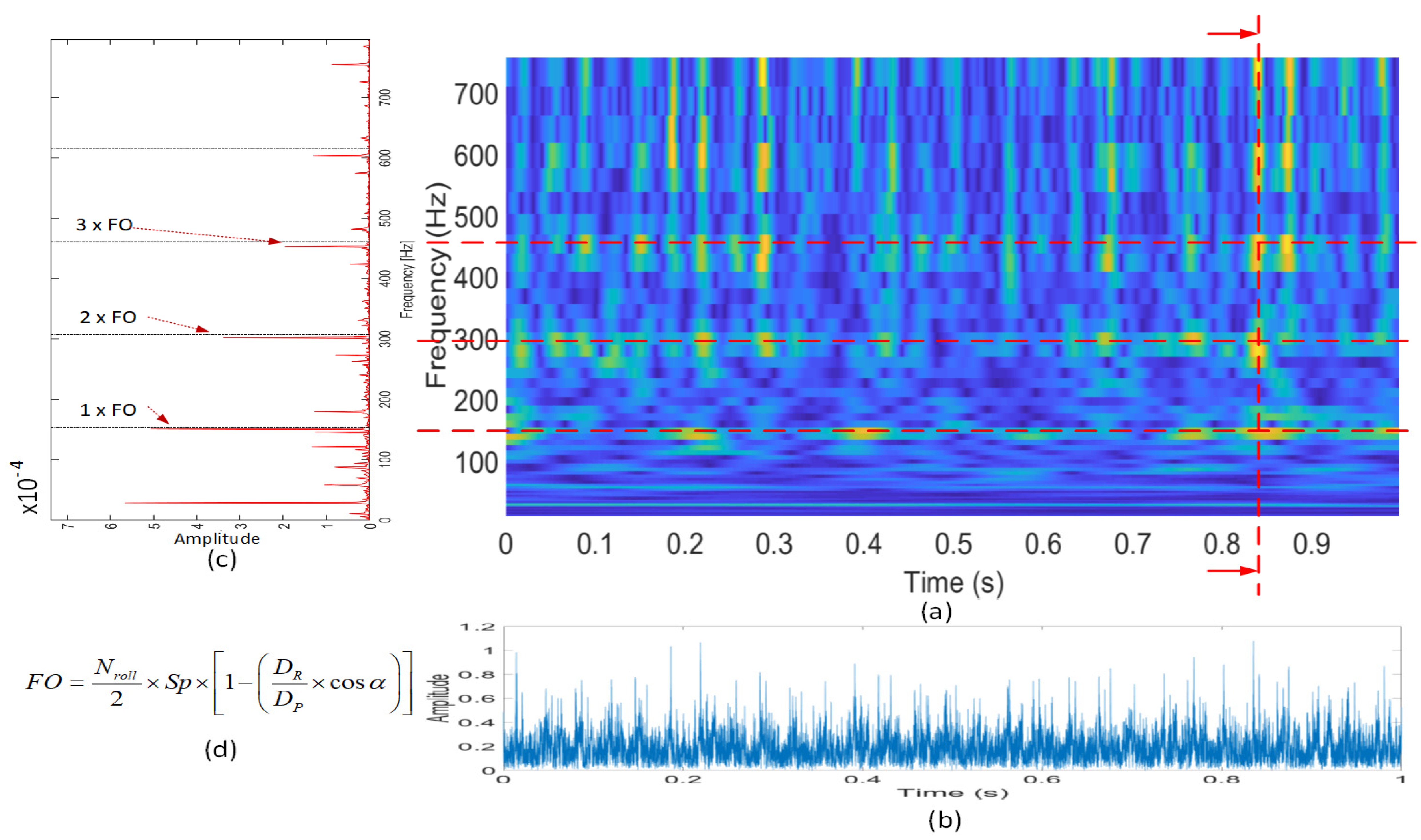
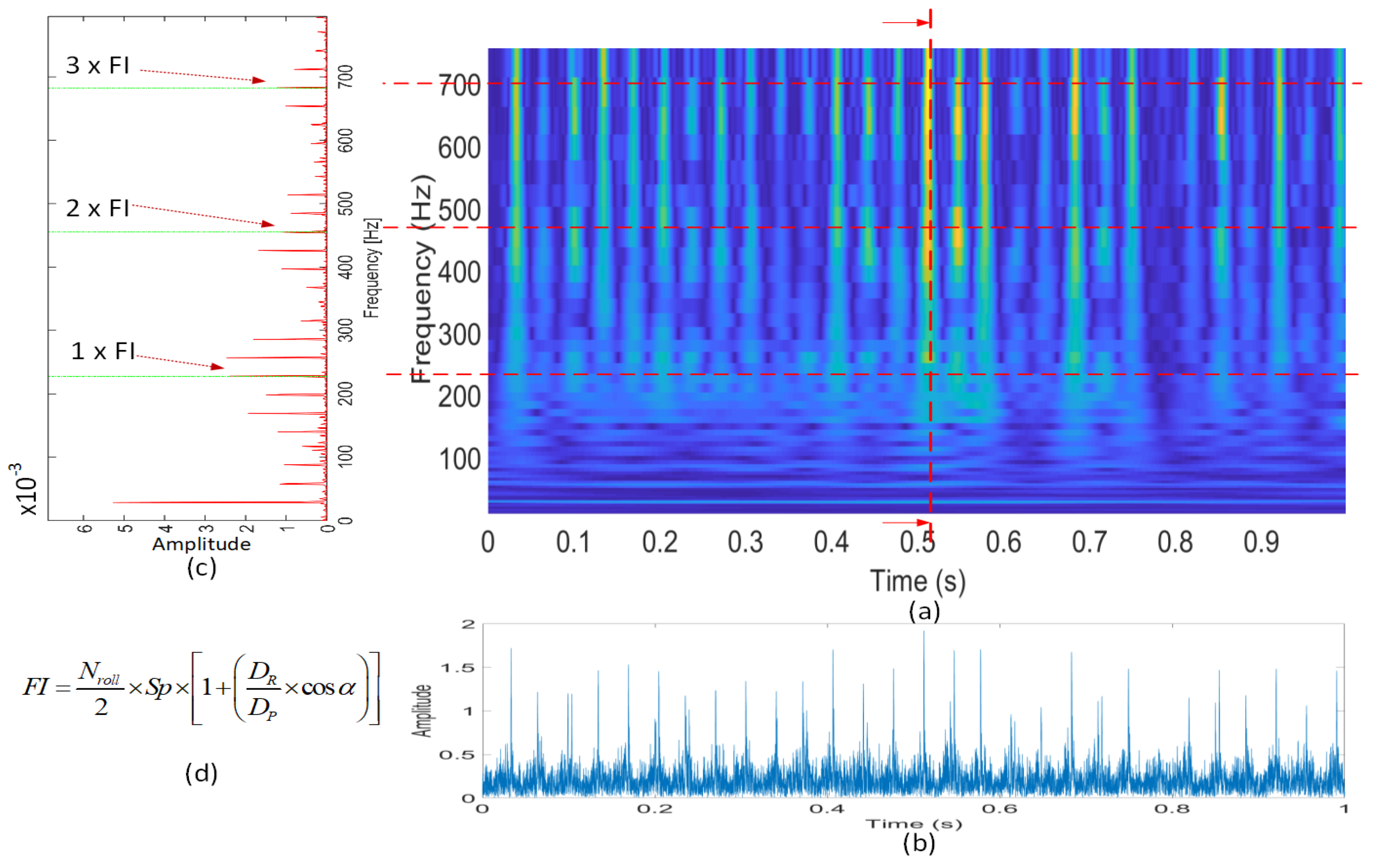
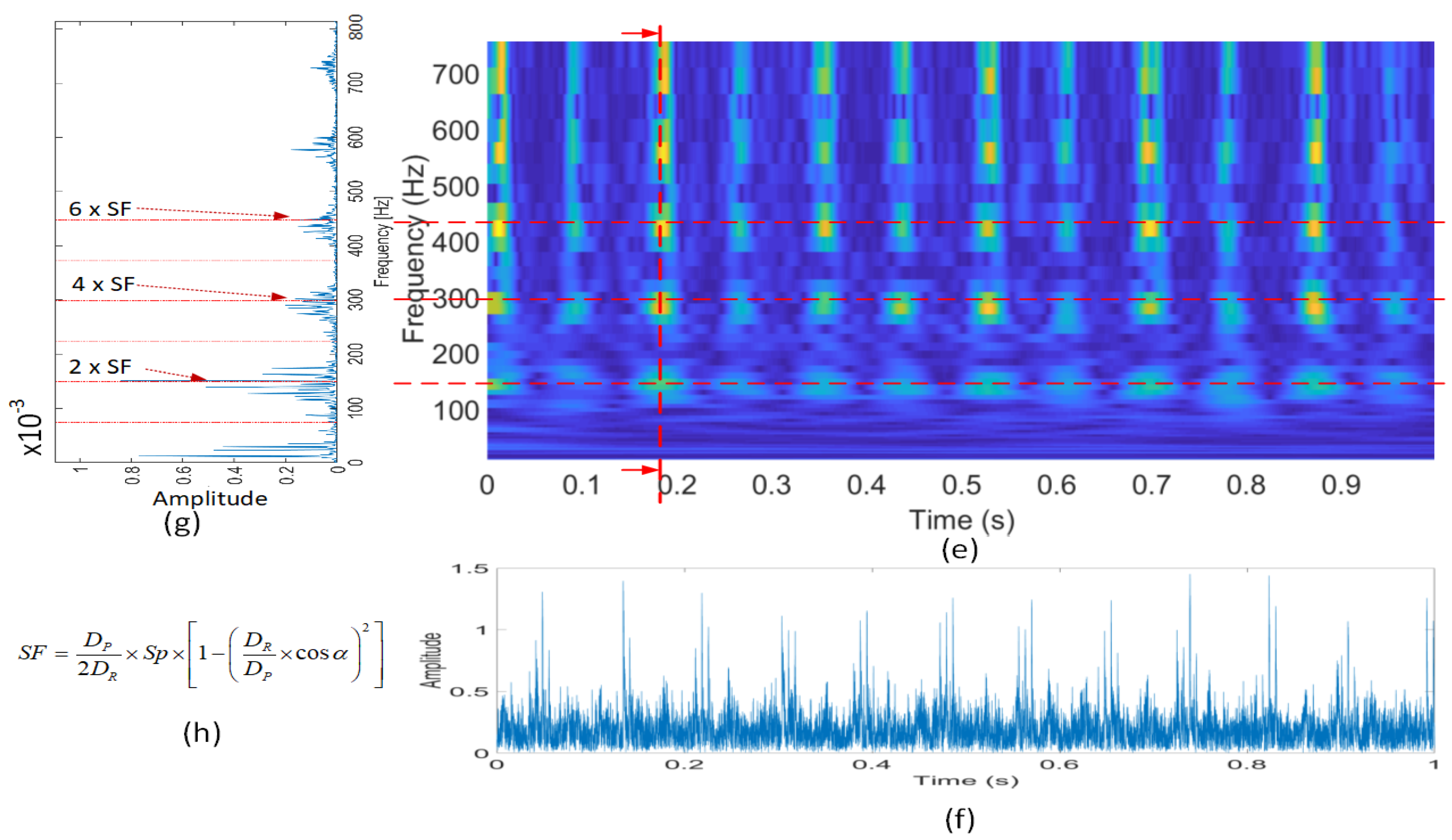
Bearing faults can occur with many types of damage presenting such as spalling, pitting, misaligned races, waviness that happens due to improper installation, abrasive wearing, manufacturing error, material fatigue, and so on. In general, the fault in each bearing element has a specific representative frequency. When the fault appears on a bearing component, the interaction of defects with other surfaces generates pulses with small duration which lead to an increasing vibrational energy at that specific frequency. These particular frequencies depend on the geometry characteristics of the bearing such as the number of rolling elements (or balls) N r o l l , the rolling element’s diameter D R , the cage diameter or pitch diameter D p , the contact angle of the balls α , and the rotational frequency S p . This phenomenon will generate a high peak at a particular position in the spectrum from the FFT analysis. However, the damage frequency is amplitude-modulated to the high-frequency region that causes indiscriminate visualization when we observe the spectrum with the conventional FFT method. To overcome this drawback, the demodulation method is used with the Hilbert transform and envelope analysis. By these methods, a signal is filtered by the bandpass filter in a frequency band in which the fault impulse is amplified by structure resonances and is applied to remove the carrier signal. The envelope signals of bearing outer, inner, and roller faults are illustrated in Figure 2b, Figure 3b, and Figure 3f, respectively. The obtained envelope signal contains richer diagnostic information both in terms of the repetition frequency of ball-bass and ball-spin frequency about bearing fault. The envelope spectra, obtained by applying the FFT to the envelope signal with specific defect frequencies FO, FI, and SF, for respective cases of outer, inner, and roller faults, are illustrated in Figure 2c and Figure 3c,g, respectively. Nevertheless, the envelope analysis still imparts some limitation. If only the FFT is used to calculate the envelope spectrum, that would lead to the loss of the time information of the signal envelope concerning the specified time when these impulses appear. To solve this issue, the authors proposed another method using the continuous wavelet transform spectrogram with a specific frequency range that covers the three harmonics of the largest defect frequency, to represent the signal envelope in both time and frequency domain.
Among the time–frequency decomposition methods, the short-time Fourier transform is constrained by the time–frequency resolution. To obtain an exact time resolution requires an analysis window to be short, whereas a long analysis window involves an accurate frequency resolution. The wavelet analysis is a recommended methodology to process the nonstationary AE signals, and it is acceptable to detect the temporary changes in the signal. In wavelet methods, the AE signals are decomposed in terms of a zero-mean function of a family of wavelets that keep an invariable shape but are able to be dilated and shifted in time. The continuous wavelet transform (or an admissible wavelet) projects an AE signal s ( t ) onto a family of zero-mean functions ψ σ , ν ( t ) (family of wavelets):
W s ( σ , ν ) = + s ( t ) ψ σ , ν * ( t ) d t ,
where ψ σ , ν * ( t ) represents the complex conjugate, σ stands for a dilation factor, and ν is a translation factor. The wavelets remain normalized, such that ψ σ , ν = 1 , as the mother wavelet is normalized. The factor ν has the role of shifting in time such that if the ν gets a positive value, the mother wavelet is shifted to the right, and if the ν gets a negative value, the mother wavelet is shifted to the left. To comprehend the role of the dilation σ in wavelet analysis, let us use Parseval’s theorem to transfer the Equation (1) to the frequency domain:
W s ( σ , ν ) = 1 2 π + s ^ ( w ) ψ ^ σ , ν * ( w ) d w ,
where s ^ ( w ) represents the Fourier transforms of s ( t ) and ψ ^ σ , ν * ( w ) are Fourier transforms of ψ σ , ν * ( t ) . Since ψ ^ ( 0 ) = 0 , the transfer function of a bandpass filter is represented by ψ ^ ( w ) , which means the function s ( t ) is particularized by the decomposition with wavelet family in the form of a series of different frequency bandwidths. Furthermore, the energy bandwidth can be expressed by:
ε w 2 = 1 2 π E 0 + ( w w c ) 2 | ψ ^ ( w ) | 2 d w ,
where w c corresponds to the center frequency of ψ ^ ( w ) , and E = ( 1 / 2 π ) 0 + | ψ ^ ( w ) | 2 d w . Hence, the center frequency of the wavelet and the energy bandwidth of the wavelet are ( w c / σ ) and ( ε w / σ ) , respectively. Thus, since the scaling parameter σ changes, both the energy bandwidth and the center frequency of the wavelet vary. That means if the value of factor σ is large, the mother wavelet has the role of a zoom-in function and vice versa. Moreover, when the value of parameter σ is large, the bandpass width becomes diminutive, which yields an increase of resolution in frequency analysis. In this paper, the 2-D representation DSWI with the CWT spectra from the envelope signal of AE signal for the outer, inner, and roller faults are shown in Figure 2a and Figure 3a,e, respectively. These figures depict the pattern considering both the frequency domain described by the defect envelope spectrum and the information from the time domain of the envelope signal which appears in the form of a periodic impulse. These figures also illustrate that depending on the amplitude of impulse and the attenuation process, these impulses cannot always be seen in the frequency spectrum. At some point, these defect frequencies can be diminished and not be seen even if this is the 1X harmonic which usually has higher energy than the others. This characteristic represents the non-stationarity of the system. Moreover, if the segment signal has a length of less than 0.1 s, the information about the bearing defects is missed. Hence, setting up the sampling rate and segment length appropriately is important to not lose the information.

3.2. 2-D Data Representation with Defect Signature Wavelet Image Generation

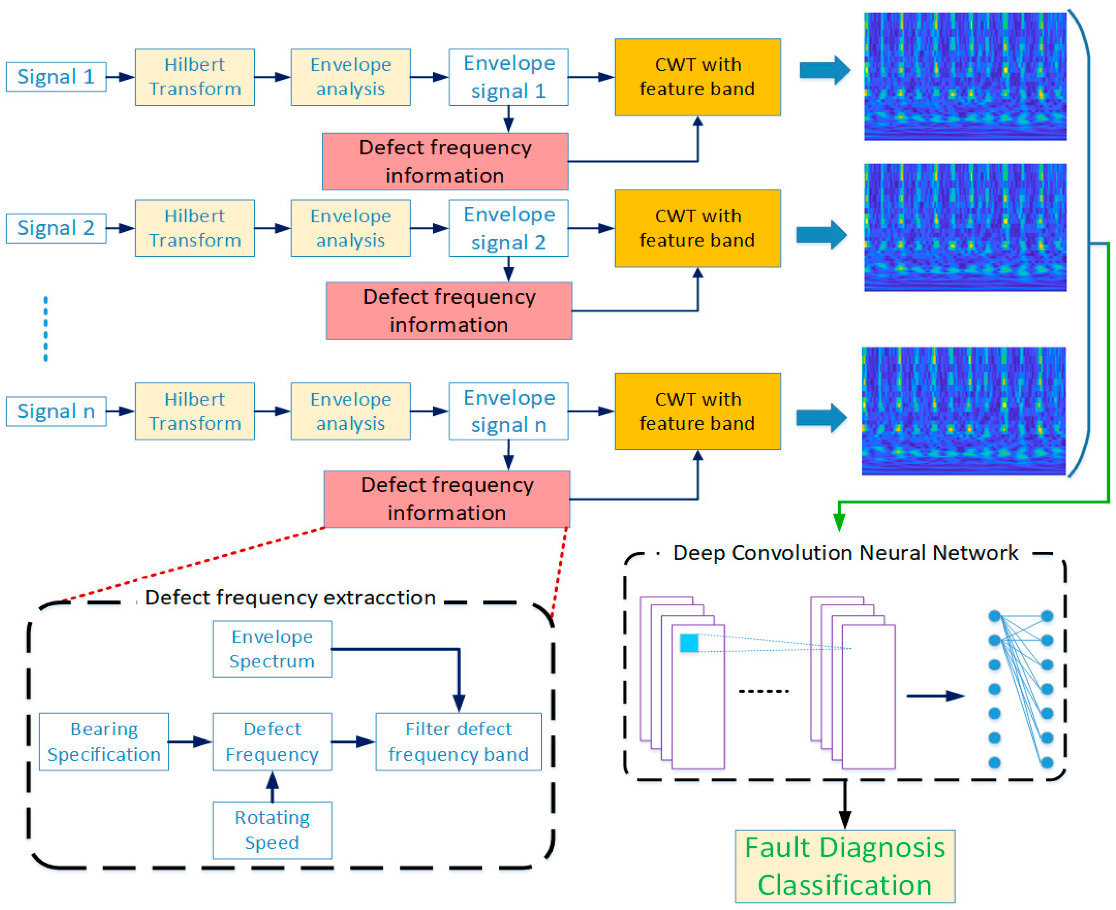
The overall process of the proposed methodology to construct the DSWI and bearing fault diagnosis is presented in Figure 4. Fundamentally, by virtue of the Hilbert transform, the signal envelope can be computed. The one-second AE signal s ( t ) in the time domain is converted to the Hilbert domain s ˜ ( t ) using the Hilbert transform [27,28]. The Hilbert transform applies the convolution of s ( t ) with the signal of 1 / π t that produces s ˜ ( t ) = s ( t ) ( 1 / π t ) . Then the method calculates the analytic signal in a complex number form with both s ( t ) in the real part and s ˜ ( t ) in the imaginary part as s a ( t ) = s ( t ) + j s ˜ ( t ) in quadrature, where j represents the imaginary unit. Immediately, an advantage is detailed in that the demodulating of the extraction of the spectrum section is effectively executed by an ideal filter, which helps to distinguish it from adjacent components which will be considerably stronger such as the gear mesh frequencies. Following that, the absolute value of e n v ( t ) = | s a ( t ) | = | s ( t ) + j s ˜ ( t ) | is computed to yield the signal envelope. Then, the square root of FFT with signal e n v ( t ) performs the envelope spectrum. In fact, it is more desirable to analyze the square of the envelope signal instead of the envelope itself. A simple argument for that is by comparison of the spectra of a squared signal with that of a rectified signal. In mathematical terms, it should be considered that a rectified signal is the same as the square root of the squared signal. Likewise, the envelope of the signal is calculated as the square root of the squared envelope. When the square root operator is applied, it launches extraneous components which do not appear in the original squared signal, and this is the reason to create the masking of the desired information. Because the entire operation is calculated digitally, it is impossible to erase the high harmonics by using lowpass filtration, and they generate the alias to the measurement range, which causes masking. In addition, when applying the one-sided spectrum, by considering the analytic signals whose squared envelope is constructed by multiplication with its complex conjugate, the spectra of the squared envelope is the convolution of the respective spectra. When this convolution is carried out, the result only yields different frequencies, e.g., sideband spacings. These different frequencies will contain the desired modulation information. Then the envelope signal is supplied to the continuous wavelet transform.
The continuous wavelet transform with damage frequency filter band is applied after obtaining the envelope signal to generate the DSWI representation. The use of wavelet transforms to detect local faults in bearings has been described by many authors. However, most of the literature on utilization of wavelet decomposition for fault diagnostics makes the error of considering the performance only in the time-domain (mostly for denoising) and on a short recorded segment of signal, frequently shorter than the longest modulation period. Usually, the assertion is that the wavelet transform is more advanced than envelope analysis. Nevertheless, many authors fail to realize that the wavelet coefficients’ squared modulus is helpful for a squared envelope signal, and much diagnostic information can be derived by analyzing the frequency domain of such squared envelope signals. As discussed, frequency-domain analysis of the envelope signal often makes evident fault repetition (in the form of transition peaks) and modulation patterns which are often difficult to recognize in time-domain signals, especially when the modulation phenomenon is so strong that the transient impulse is only stimulated when the fault point is inside the load-zone. These impulses are thus created with greatly varied amplitude. For instance, the continuous wavelet transform has a similar skeleton with the Fourier transform. While the Fourier transform yields correlation coefficients between the original signal and a sinusoidal signal, continuous wavelet transform obtains correlation coefficients resulting from an inner product of the mother wavelet and the signal. Unlike the Fourier transform though, where the signal is converted into the frequency-domain, continuous wavelet transform transfers the signal to the time-frequency-domain by managing the shape of the mother wavelet. Here, the research controls the shape of the mother wavelet by adjusting the scaling and shifting parameters. Continuous wavelet transform, using a smooth analytical mother wavelet, is able to identify the dynamic frequency characteristics of the signal at different scales. By employing various dilates and translations to the mother wavelet function, continuous wavelet transform coefficients reflect the resemblance of the signal to the wavelet at the current scale. The bump wavelet is a good choice for the continuous wavelet transform when signals are oscillatory, and when the researchers are more interested in time-frequency analysis than in the localization of transients. Moreover, bump wavelet has the best time resolution permitting separation of the start and the end times for each component of the signal with impressive precision for each of the performed tests. The bump is the symmetric wavelet in frequency and has an immediate relationship between the scale and the center frequency. The bump wavelet is defined by:
ψ ^ b u m p ( ζ ) = e 1 1 1 σ 2 ( ζ ν ) 2 χ ( ν 1 / σ , ν + 1 / σ ) ( ζ )
where σ > 0 , ν > 0 with σ ν > 1 , are the commonly used with continuous wavelets. The parameter σ controls the window widths of the time-frequency localization of the wavelets (plays a role in trans-shaping the mother wavelet ψ b u m p ) and has effects on the representation of the transformed signal. In the literature, the wavelet parameter σ is usually treated as a fixed constant. The bump wavelet ψ b u m p is bandlimited and hence it has better frequency localization than other wavelet families. ζ ψ = ν admits the peak frequency which is defined by ζ ψ : = arg max ζ | ψ b u m p ( ζ ) | and χ denotes the indicator function. The translation parameter ν is involved in the mother wavelet’s location and specifies the properties of the resulting child wavelets. Therefore, this research also determines the characteristic signature of faults at various locations of the mother wavelet by controlling the translation. The high-resolution in the frequency of large-scale wavelet permits us to capture the harmonic of the slow-variation elements whenever the fine-resolution of time in small-scale wavelet allows us to catch the fast-variation elements in the AE data. The wavelet decomposition enables detection of the hidden details of transient impulse waveforms, which is significant for inspecting a signal which contains both high frequency and low frequency components. In the case of the bump wavelet, the wavelet representation is almost symmetric with respect to the scale associated with the peak frequency. Since most defect characteristic harmonics stay in the low frequency range, fine-resolution frequency band analysis is essential to exactly interpret the properties of the abnormal indications in the bearing. As mentioned previously, the mother wavelet works in the role of a bandpass filter that permits a special frequency band to pass across a range existing between two limiting frequencies. This paper scrutinized the multiple faults which occur in bearings by changing the cutoff frequencies of the bandpass filter with the frequency range which contains defect characteristics. The matrix of wavelet coefficients is established with the wavelet coefficients in a range which is defined as below:
P i , j = f ( ω ) with   ω   = 0 . . f max   and   f max = max ( F O , F I , S F ) × k + f s i d e
where k is the number of considered harmonics and f s i d e is the sideband of the highest defect frequency. Moreover, the initial low cutoff frequency is set to zero hertz for the fine resolution analyses in frequency. Because the frequency range is the function of rotation speed, it is robust when the rotating speed changes. Therefore, the DWSI always contains the damage frequency harmonics of bearing faults. Using these settings, the 2-D coordinate matrices are constructed, and then the values of coefficients in the matrix are employed to define the vertex colors by scaling the values in the matrix to the full range of the colormap to convert the representation of a 1-D vibration signal as a 2-D spectrogram image. Then, the 2-D which is similar to the spectrogram image is fed to a DCNN model which is designed and trained for feature learning and classification.

3.3. Deep Convolution Neural Network Structure Specification

Convolution neural network has several benefits comparable to other feature-learning methodologies. Previously, much as the stacked sparse auto-encoder did, the CNN automatically learns numerous levels of abstract representations from the data via their deep architecture layers. The learning process enables signals of high complexity to be learned to create a high-order representation feature. Secondly, the CNN applies an end-to-end structure for the learning model, hence, a single unique structure has to be optimized and the testing phase only needs a one-pass feed-forward process. Finally, the CNN model is utilized to exploit the spatial characteristic in the constructed DSWI from the sensor data. By using the sparse number of attributes, CNN reduces the number of training parameters when compared to the multi-layer perceptron network (a conventional artificial neural network). In the case of a DSWI from the AE signal, the DCNN defines a spatial architecture as the set of three channels with respect to three channels of the DSWI. A typical case to note is that due to the rolling and sliding mode combination of the roller or ball in bearing, the expected energy which is contained in a fundamental frequency may not totally appear in the frequency range close to the fundamental frequency. Therefore, deploying this information can ameliorate the performance of the fault detection algorithm. Instead of feature extraction stage with the features being designed by experts, it should be considered that the difference of feature-learning method is in the researched work of this paper as here, the feature extraction stage is not employed; thus, the DCNN model is directly implemented on the DSWI of the AE data so that the DCNN has the capacity to learn the features itself. Many optimization constraints, comprising batch normalization, dropout, initialization methods, and leaky rectified linear units, are also used for incorporating into the principal architecture of the DCNN to create better classification performance. A DCNN operates as follows: given an input image consisting of multiple channels, a convolutional layer computes a transformed output as the function of the input, weights and bias parameters, with the difference from the normal artificial neural network being that the adjusted variables of the layer are organized as a sequence of filters and are applied to the convolving operator over the input to produce the output of the convolution layer. Each convolutional layer output is a 3D tensor, which includes a stack of 2-D matrices, the so-called feature maps, which will be utilized as input to feed to the next network layer of the DCNN model. The weight parameters in the filter bank are distributed and shared over the local region of input, which efficaciously exploits the local spatial characteristics, and also diminishes the quantity of optimized parameters. The convolutional operation can be described as:
O i ( m ) = φ ( c = 1 C W i ( c , m ) S i 1 ( c ) + B i ( m ) )
In this formula, i stands for the order of the layer as before. The 2D convolution of the input S i 1 and the weight W i ( c , m ) , which is responsible for yielding m t h output of the map, is presented by the ( ) operator in the formula. The term B i ( m ) represents the bias vector. After that, we apply a nonlinear activation function φ on the sum of convolutions plus a bias vector to obtain the final output. By utilizing a deep architecture, a network with several convolution layers, the model is more robust to complex variations in the data. Thus, if the data naturally describe many variations with high complexity, a deep architecture is necessary. In the case of bearing faults, due to the manifestation of the various faults which are considered here that illustrate a little variation, a reasonably designed deep model suffices. In addition, the initial layers of CNNs learn the fastest, so a short training period is adequate to achieve convergence. A lot of variations of the proposed DCNN were examined by varying the number of convolutional blocks and fully connected layers, and the number of nodes in each layer. Applying to this particular case with the fault in bearing, an extremely deep version of the network model does not give better results but does increase the time for training. The structure which is applied in this research leverages the capacity of the DCNN for exploiting the spatial structure in the DSWI data to sufficiently capture the properties of the AE signals. After the convolutional layer, batch normalization follows to improve the convergence process by regularizing the model to avoid overfitting. Then the output from the batch normalization is fed to the nonlinear activation function. The proposed DCNN has a structure including several convolution blocks. Each block indicates one feature learning step with a specific level that includes convolution, batch-normalization, and activation function. Figure 5 depicts the designed architecture for each convolution block of the DCNN model, which consists of six blocks of convolution with filters 3–8, 8–16, 16–16, 16–8, 8–8, and 8–1. The input image has a size of 128 × 128 pixels with three channels. At the output after the six blocks, the feature maps are flattened and fed to the fully connected layers. There are two fully connected layers and a soft-max layer which has the role of the classifier. The most regularly applied non-linear activation functions are the sigmoid, hyperbolic tangent, and rectified linear units (ReLU). Among them the ReLU function has been demonstrated to be more powerful than the others. However, during the training phase, ReLU units can die, and this problem can happen when great values of gradient flow across the ReLU function. This inspires the weights to be updated, and later the ReLU neuron fails to activate ever again on any data point. The leaky-ReLU function is an improved version that attempts to address this issue. The leaky-ReLU is used to introduce non-linearity into each stage, permitting the DCNN to learn complex models. Normally, the pooling layer is employed to decrease the resolution of the feature maps via the subsampling step to reduce the number of parameters and quicken the computation. In this study, instead of using pooling to reduce the size of spatial representation, the authors proposed using the convolution layer with a large kernel size and strike. This approach shows better performance when extracting the features of the image in a deep network.
The training phase of the DCNN model relates the learning of all the weights and biases, and it is essential to obtain the optimized parameters for a successful feature learning. During the training phase of the network’s parameters, it is also necessary for the DCNN to optimize the hyperparameters, which include the learning rate and dropout. The dropout holds an important characteristic of DCNN, which considerably helps to prevent the overfitting phenomenon by generalizing the model. In the designed model, dropout with a proportion of 0.5 is employed for better regularization of the DCNN. The adapted moment estimation (Adam), which is defined as a back-propagation strategy, is utilized to control the learning rate and other hyperparameters. The Adam optimization calculates the learning rate scale for different layers and avoids manual assignment to choose a suitable learning rate. Several configurations of the deep network, including LeNet-5 [29] and AlexNet [30], were tested to compare the results with the proposed. The DCNN model was trained with minibatch gradient descent and in each minibatch 100 training examples were used. The proposed DCNN model training process is run over 100 epochs to learn the robust features for one normal operating condition and each type of faulty condition.

4. Methodology Evaluation Results

In this section, the proposed bearing fault diagnostic method is evaluated using collected data from a real-bearing testbed which is described in Section 2. The AE signal has a duration of one second for each sample. It has been shown that a proper signal processing technique is required for converting the signal to meaningful information with the DWSI before feeding to the DCNN. Each DSWI is constructed from a one-second sample signal using the method detailed in Section 3. This processing step is employed to retain the specific properties of different health states. Hence, the invariant signatures of different health conditions can use the full potential of the DCNN. Then, the DCNN model is trained to automatically extract and learn the features from 988 samples of the training dataset. The DCNN is simultaneously validated with 248 samples of the validation dataset during each iteration epoch. The trained CNN model is validated by predicting the class for 248 samples from the test dataset. To evaluate the proposed method by comparing to other methods, two scenarios were employed using different types of 2-D representations as the input and with different DCNN structures proposed in the literature.

4.1. Performance Evaluation of DSWI Compared to Vibration Image and Conventional Wavelet Spectrogram

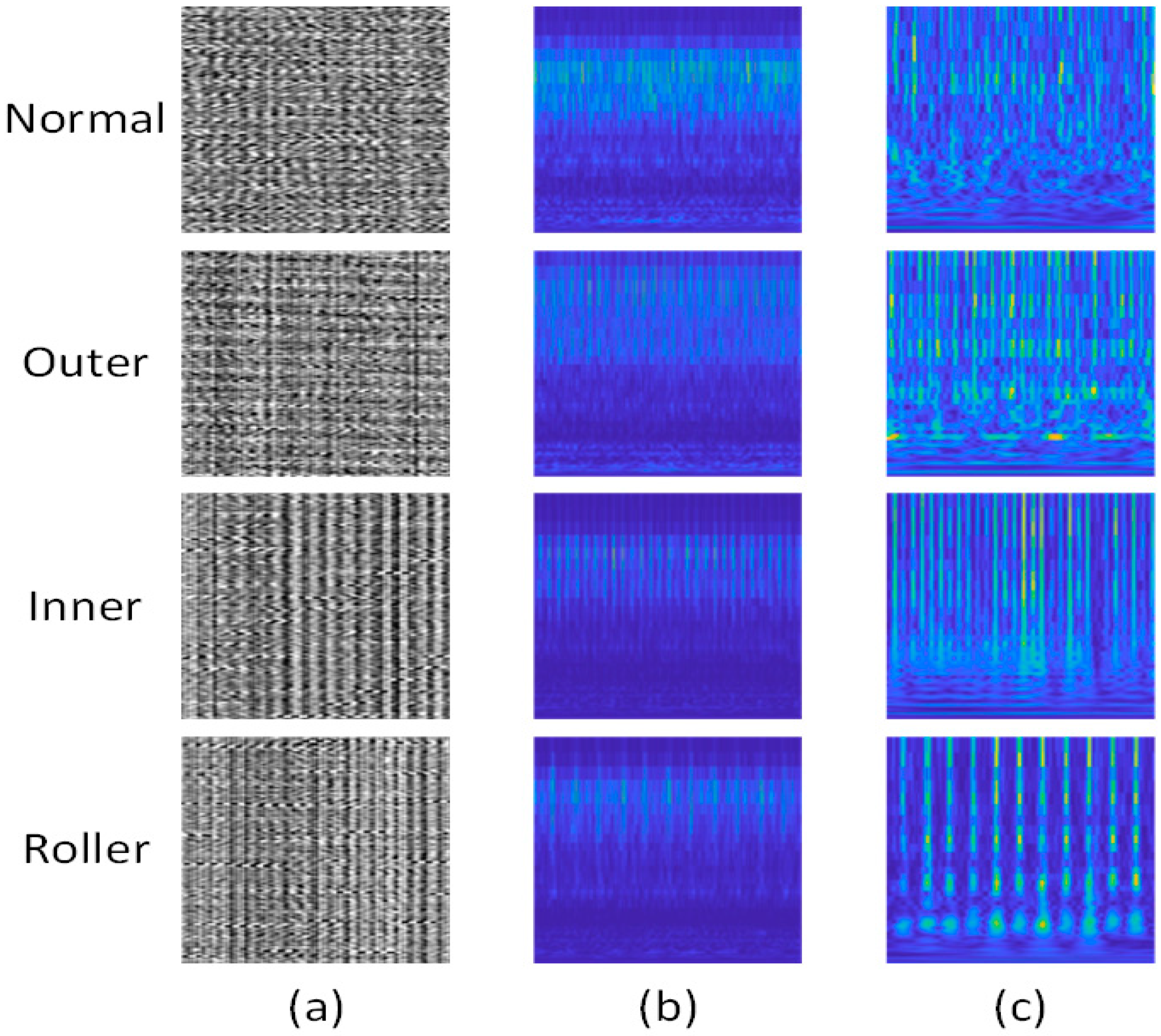
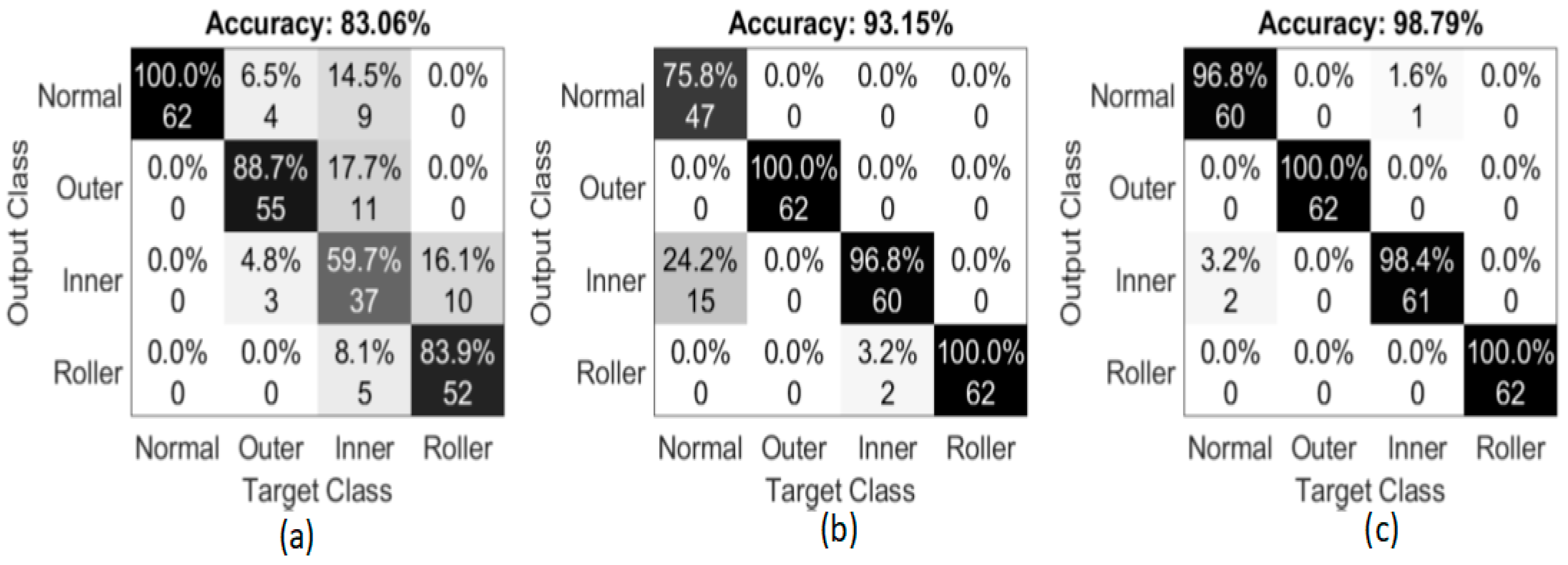
The same sample signals are used to create 2-D representations with the vibration image method and the conventional wavelet spectrogram. The vibration image is constructed by segmenting the raw signal in the time-domain into smaller samples and the segments are stacked one by one to generate the 2-D matrix. Then the values of the matrix are normalized in range [ 0 , 255 ] and converted to a grayscale image. This method is also used in [10,11] to generate the 2-D image from the vibration signal. The second method to compare with the proposed method is the conventional wavelet spectrogram. The AE signal is directly analyzed with the continuous wavelet transform without envelope analysis and the information of the damage frequency band is used to create the wavelet spectrogram. The detailed visualization of vibration image, wavelet spectrogram, and the DSWI for different types of faults in bearings and the normal case is shown in Figure 6. The proposed method with DSWI shows the pattern differences more distinctly between different types of signals compared to other 2-D representations. The other patterns do not show clearly separate visualizations from the different bearing status AE signals. Moreover, the pattern of DSWI illustrates a correlation to the damage frequencies as ascertained in Section 3. Since the AE-based method becomes more sensitive to low energy emissions from the bearing, gathering separate visual information associated with the energy distribution through low amplitudes can supply useful knowledge to further analyze. The DSWI with time-frequency-domain analysis can catch these small changes in signal form of the image by highlighting the powerful energy bands. Therefore, the DSWI includes low energy information in the field of time-frequency-domain. These kinds of images are provided as the input to the DCNN to indirectly evaluate the performance of the proposed approach through the classification accuracy. The classification accuracy performance is detailed by the confusion matrices as illustrated in Figure 7. The confusion matrix indicates the class distinguishing performance by calculating the actual versus predicted deviation. For validating the diagnostic result, the metrics of sensitivity score (SS) and mean per class of sensitivity score are used. The sensitivity score formula is presented as follows:
S S = # t r u e _ p o s # t r u e _ p o s + # f a l s e _ n e g × 100 %
Here, the term # t r u e _ p o s depicts the number of correctly predicted data samples from the provided test dataset which are used to validate the model at each iteration, and the term # f a l s e _ n e g refers to the number of data samples from a class that are wrongly classified. Hence, the average sensitivity can be obtained by a v g S S = ( S S ) / # c l a s s , where S S represents a summation of the class-wise sensitivity score for all the test dataset.
Then, the averages of all the accuracies and losses are collected to observe the accuracy values and loss values during the training stage. The DCNN model hit an accuracy of 98.79% on average with the scenario of using the DSWI as the input, while the other scenarios of using the vibration image and conventional wavelet spectrogram had average accuracies of 83.06% and 93.15%, respectively, as described in Figure 7. Other devices such as motors and the noisy factory environment create impulses or random fluctuation peaks in the AE signal making the time-domain or frequency-domain analysis inefficient for this kind of AE signal. Processing the AE signal with DWSI can, however, partly alleviate the noisy random fluctuations and environmental stimulation in the AE signal. Apart from the comparison, vibration images obtained from the time-domain analysis are not sensitive enough to weak incipient damage that may cause less discriminate information. Thus, the proper processing methods are preferred, which can result in discriminating information with conventional wavelet spectrogram and DSWI. From performances that are based on the other methods of the 2-D converted image of the AE signal, which taken together with results in discriminant patterns form for different types of faults in bearings, the conventional wavelet spectrogram can obtain a classification accuracy of more than 90%. However, the proportion of misclassification among different class types is not equal. Most of the misclassification happens in normal class because the pattern is not sufficiently discriminant. From the classification report, it is clearly observable that the proposed DCNN model with the DSWI input is able to extract and learn the features from the training dataset and classify the features in the testing dataset for the appropriate faulty and healthy conditions.

4.2. Performance Comparison with Difference Model for Classification

To further validate the performance of the diagnostic method, the proposed DCNN model is compared against several state-of-the-art approaches: (1) K-nearest-neighbor + principal component analysis (KNN+PCA), (2) Multiclass Support Vector Machines + principal component analysis (MCSVM+PCA), (3) LeNet-5, and (4) AlexNet. The KNN and SVM methods using the feature extraction (FE)-based approach where the features are texture features extracted from the images of different types of 2-D representation include vibration image, conventional wavelet spectrogram and the proposed of DSWI. These features are extracted using the uniform local binary pattern method [31]. The method is employed based on the concept of the certain local binary patterns, termed uniform, that are fundamental characteristics of local image texture. The image’s occurrence histogram is indicated to be a very useful texture feature. Then, the KNN or MCSVM algorithm is utilized to carry out the fault classification after decreasing the feature space’s dimensionality by principal component analysis. The LeNet-5 and AlexNet are two well-known CNN structures commonly used in the literature for image processing. The input of the LeNet-5 and AlexNet is the vibration image, the conventional wavelet spectrogram and the DSWI analogous to the input of the proposed DCNN. The experiment comparing the DCNN with the other approaches in literature is conducted with the same dataset that is used to evaluate the proposed model. The recorded dataset used to evaluate the proposed DCNN and other machine learning models is detailed in Section 2. The prediction accuracy for the testing part of the dataset for each implemented method is gathered and presented in Table 2. As can be seen from Table 2, the other 2-D representation methods (i.e., vibration image and conventional wavelet spectrogram) showed inferior fault diagnostic performance when compared to the DSWI approach employed for the signal processing step. Thus, the comparison results show that the proposed DSWI clearly outperformed the other types of 2-D representations for all experimental scenarios with different classifier methods.
Table 2 also presents a collation of the other classifier models that are investigated with the proposed DCNN. Therefore, by comparison with the recently researched deep learning architectures, our approach provides a better result. The results show that the proposed DCNN approach attains a result superior to that of the other methods. The prediction accuracy is 98.79%, 97.98%, 95.97%, 87.76% and 61.63% for proposed DCNN, AlexNet and LeNet-5, MCSVM+PCA, and KNN + PCA, respectively. This result also shows the superior performance of the proposed DCNN approach. For the KNN + PCA and MCSVM + PCA which are based on the feature extraction method, the results illustrate lower accuracy because they depend on the characteristic of features, while the design of features needs the help of the experts for different types of application. The results from the LeNet-5 and AlexNet showed high accuracies proximate to the proposed DCNN. However, the LeNet-5 is the simplest architecture and is not a strong enough structure for learning the information from the DSWI which is highly complex. AlexNet gives a better result but it is more complex and requires more time spent on training. According to the results reported in Table 2, the diagnostic performance of the DCNN is best in all scenarios.

5. Conclusions

In the modern era, the high complexity industrial system can ensure reliability and safety thanks to the sensor devices that have become necessary modules in comprehensive systems. Acoustic emission signals have emerged as an intelligent and optimized solution that simplifies the fault diagnostic procedure with a sequence of sensors. In this study, da ata-driven methodology using an acoustic emission signal analyzed by envelope analysis and an enhanced continuous wavelet transform with the damage frequency band information was used to generate the new 2-D representation image (so-called DSWI) from the 1-D signal. This DSWI shows the discriminate pattern and correlates with the defect frequencies for each type of fault in bearings helping to improve the performance of the machine learning methods for bearing fault diagnosis. The purpose of this study is also to propose a DCNN architecture that is suitable for separating the DSWI from different types of faults in bearing. To validate the diagnostic result of the proposed approach, the data collected from an elaborately self-designed testbed are deployed. Then, the experimental findings imply that the DCNN classifiers achieved greater than 98% accuracy and other evaluation parameters also outperformed the current state-of-the-art. By incorporating the deep learning-based structure with the new time-frequency domain-based 2-D representation, the proposed method is efficacious, with great accuracy and no need for the feature selection stage. In addition, a collated comparison with some well-known methods in literature is executed and indicates that the DSWI with the DCNN algorithm can become a promising method for bearing fault diagnosis.

Author Contributions

All of the authors contributed equally to the conception of the idea, the design of experiments, the analysis and interpretation of results, and the writing and improvement of the manuscript. All authors have read and agreed to the published version of the manuscript.

Funding

This work was supported by the Technology Infrastructure Program funded by the Ministry of SMEs and Startups (MSS, Korea). This research was also financially supported by the Ministry of Trade, Industry & Energy (MOTIE) of the Republic of Korea and Korea Institute for Advancement of Technology (KIAT) through the Encouragement Program for The Industries of Economic Cooperation Region (P0002312).

Conflicts of Interest

The authors declare no conflict of interest.

References

  1. Lau, E.C.C.; Ngan, H.W. Detection of Motor Bearing Outer Raceway Defect by Wavelet Packet Transformed Motor Current Signature Analysis. IEEE Trans. Instrum. Meas. 2010, 59, 2683–2690. [Google Scholar] [CrossRef]
  2. Nishat Toma, R.; Kim, J.-M. Bearing Fault Classification of Induction Motors Using Discrete Wavelet Transform and Ensemble Machine Learning Algorithms. Appl. Sci. 2020, 10, 5251. [Google Scholar] [CrossRef]
  3. Gao, Z.; Cecati, C.; Ding, S.X. A Survey of Fault Diagnosis and Fault-Tolerant Techniques—Part I: Fault Diagnosis With Model-Based and Signal-Based Approaches. IEEE Trans. Ind. Electron. 2015, 62, 3757–3767. [Google Scholar] [CrossRef] [Green Version]
  4. Gao, Z.; Cecati, C.; Ding, S.X. A Survey of Fault Diagnosis and Fault-Tolerant Techniques—Part II: Fault Diagnosis With Knowledge-Based and Hybrid/Active Approaches. IEEE Trans. Ind. Electron. 2015, 62, 3768–3774. [Google Scholar] [CrossRef]
  5. Prosvirin, A.E.; Piltan, F.; Kim, J.-M. Hybrid Rubbing Fault Identification Using a Deep Learning-Based Observation Technique. IEEE Trans. Neural Netw. Learn. Syst. 2020, 32, 1–12. [Google Scholar] [CrossRef]
  6. Piltan, F.; Kim, J.-M. Bearing Fault Diagnosis Using an Extended Variable Structure Feedback Linearization Observer. Sensors 2018, 18, 4359. [Google Scholar] [CrossRef] [PubMed] [Green Version]
  7. Piltan, F.; Prosvirin, A.E.; Jeong, I.; Im, K.; Kim, J.-M. Rolling-Element Bearing Fault Diagnosis Using Advanced Machine Learning-Based Observer. Appl. Sci. 2019, 9, 5404. [Google Scholar] [CrossRef] [Green Version]
  8. Kang, M.; Kim, J.; Wills, L.M.; Kim, J.-M. Time-Varying and Multiresolution Envelope Analysis and Discriminative Feature Analysis for Bearing Fault Diagnosis. IEEE Trans. Ind. Electron. 2015, 62, 7749–7761. [Google Scholar] [CrossRef]
  9. Manjurul Islam, M.M.; Kim, J.-M. Reliable multiple combined fault diagnosis of bearings using heterogeneous feature models and multiclass support vector Machines. Reliab. Eng. Syst. Saf. 2019, 184, 55–66. [Google Scholar] [CrossRef]
  10. Do, V.T.; Chong, U.-P. Signal Model-Based Fault Detection and Diagnosis for Induction Motors Using Features of Vibration Signal in Two- Dimension Domain. J. Mech. Eng. 2011, 57, 655–666. [Google Scholar] [CrossRef]
  11. Wen, L.; Li, X.; Gao, L.; Zhang, Y. A New Convolutional Neural Network-Based Data-Driven Fault Diagnosis Method. IEEE Trans. Ind. Electron. 2018, 65, 5990–5998. [Google Scholar] [CrossRef]
  12. Tra, V.; Khan, S.A.; Kim, J.-M. Diagnosis of bearing defects under variable speed conditions using energy distribution maps of acoustic emission spectra and convolutional neural networks. J. Acoust. Soc. Am. 2018, 144, EL322–EL327. [Google Scholar] [CrossRef] [PubMed]
  13. Sohaib, M.; Kim, J.-M. Fault Diagnosis of Rotary Machine Bearings under Inconsistent Working Conditions. IEEE Trans. Instrum. Meas. 2020, 69, 3334–3347. [Google Scholar] [CrossRef]
  14. Hasan, M.J.; Kim, J.-M. Bearing Fault Diagnosis under Variable Rotational Speeds Using Stockwell Transform-Based Vibration Imaging and Transfer Learning. Appl. Sci. 2018, 8, 2357. [Google Scholar] [CrossRef] [Green Version]
  15. Cai, J.; Xiao, Y. Time-frequency analysis method of bearing fault diagnosis based on the generalized S transformation. J. Vibroeng. 2017, 19, 4221–4230. [Google Scholar] [CrossRef]
  16. Pham, M.T.; Kim, J.-M.; Kim, C.H. Accurate Bearing Fault Diagnosis under Variable Shaft Speed using Convolutional Neural Networks and Vibration Spectrogram. Appl. Sci. 2020, 10, 6385. [Google Scholar] [CrossRef]
  17. Huang, W.; Gao, G.; Li, N.; Jiang, X.; Zhu, Z. Time-Frequency Squeezing and Generalized Demodulation Combined for Variable Speed Bearing Fault Diagnosis. IEEE Trans. Instrum. Meas. 2019, 68, 2819–2829. [Google Scholar] [CrossRef]
  18. Tse, P.W.; Yang, W.; Tam, H.Y. Machine fault diagnosis through an effective exact wavelet analysis. J. Sound Vib. 2004, 277, 1005–1024. [Google Scholar] [CrossRef]
  19. Bessous, N.; Zouzou, S.E.; Bentrah, W.; Sbaa, S.; Sahraoui, M. Diagnosis of bearing defects in induction motors using discrete wavelet transform. Int. J. Syst. Assur. Eng. Manag. 2018, 9, 335–343. [Google Scholar] [CrossRef]
  20. Zhang, X.; Liu, Z.; Wang, J.; Wang, J. Time–frequency analysis for bearing fault diagnosis using multiple Q-factor Gabor wavelets. ISA Trans. 2019, 87, 225–234. [Google Scholar] [CrossRef]
  21. Randall, R.B.; Antoni, J. Rolling element bearing diagnostics—A tutorial. Mech. Syst. Signal Process. 2011, 25, 485–520. [Google Scholar] [CrossRef]
  22. Ben Ali, J.; Fnaiech, N.; Saidi, L.; Chebel-Morello, B.; Fnaiech, F. Application of empirical mode decomposition and artificial neural network for automatic bearing fault diagnosis based on vibration signals. Appl. Acoust. 2015, 89, 16–27. [Google Scholar] [CrossRef]
  23. Janssens, O.; Slavkovikj, V.; Vervisch, B.; Stockman, K.; Loccufier, M.; Verstockt, S.; Van de Walle, R.; Van Hoecke, S. Convolutional Neural Network Based Fault Detection for Rotating Machinery. J. Sound Vib. 2016, 377, 331–345. [Google Scholar] [CrossRef]
  24. Duong, B.P.; Kim, J.-M. Non-Mutually Exclusive Deep Neural Network Classifier for Combined Modes of Bearing Fault Diagnosis. Sensors 2018, 18, 1129. [Google Scholar] [CrossRef] [PubMed] [Green Version]
  25. R15I-AST—150 kHz Integral Preamp AE Sensor. Available online: https://www.physicalacoustics.com/by-product/sensors/R15I-AST-150-kHz-Integral-Preamp-AE-Sensor (accessed on 18 October 2020).
  26. PCB Model 622B01. Available online: https://www.pcb.com/products?model=622B01&item_id=Products&m=052BR030BZ (accessed on 18 October 2020).
  27. Wang, D.; Miao, Q.; Fan, X.; Huang, H.-Z. Rolling element bearing fault detection using an improved combination of Hilbert and wavelet transforms. J. Mech. Sci. Technol. 2009, 23, 3292–3301. [Google Scholar] [CrossRef]
  28. Kang, M.; Kim, J.; Kim, J.-M. High-Performance and Energy-Efficient Fault Diagnosis Using Effective Envelope Analysis and Denoising on a General-Purpose Graphics Processing Unit. IEEE Trans. Power Electron. 2015, 30, 2763–2776. [Google Scholar] [CrossRef]
  29. LeCun, Y.; Boser, B.; Denker, J.S.; Henderson, D.; Howard, R.E.; Hubbard, W.; Jackel, L.D. Backpropagation Applied to Handwritten Zip Code Recognition. Neural Comput. 1989, 1, 541–551. [Google Scholar] [CrossRef]
  30. Krizhevsky, A.; Sutskever, I.; Hinton, G.E. ImageNet classification with deep convolutional neural networks. Commun. ACM 2017, 60, 84–90. [Google Scholar] [CrossRef]
  31. Ojala, T.; Pietikainen, M.; Maenpaa, T. Multiresolution gray-scale and rotation invariant texture classification with local binary patterns. IEEE Trans. Pattern Anal. Mach. Intell. 2002, 24, 971–987. [Google Scholar] [CrossRef]
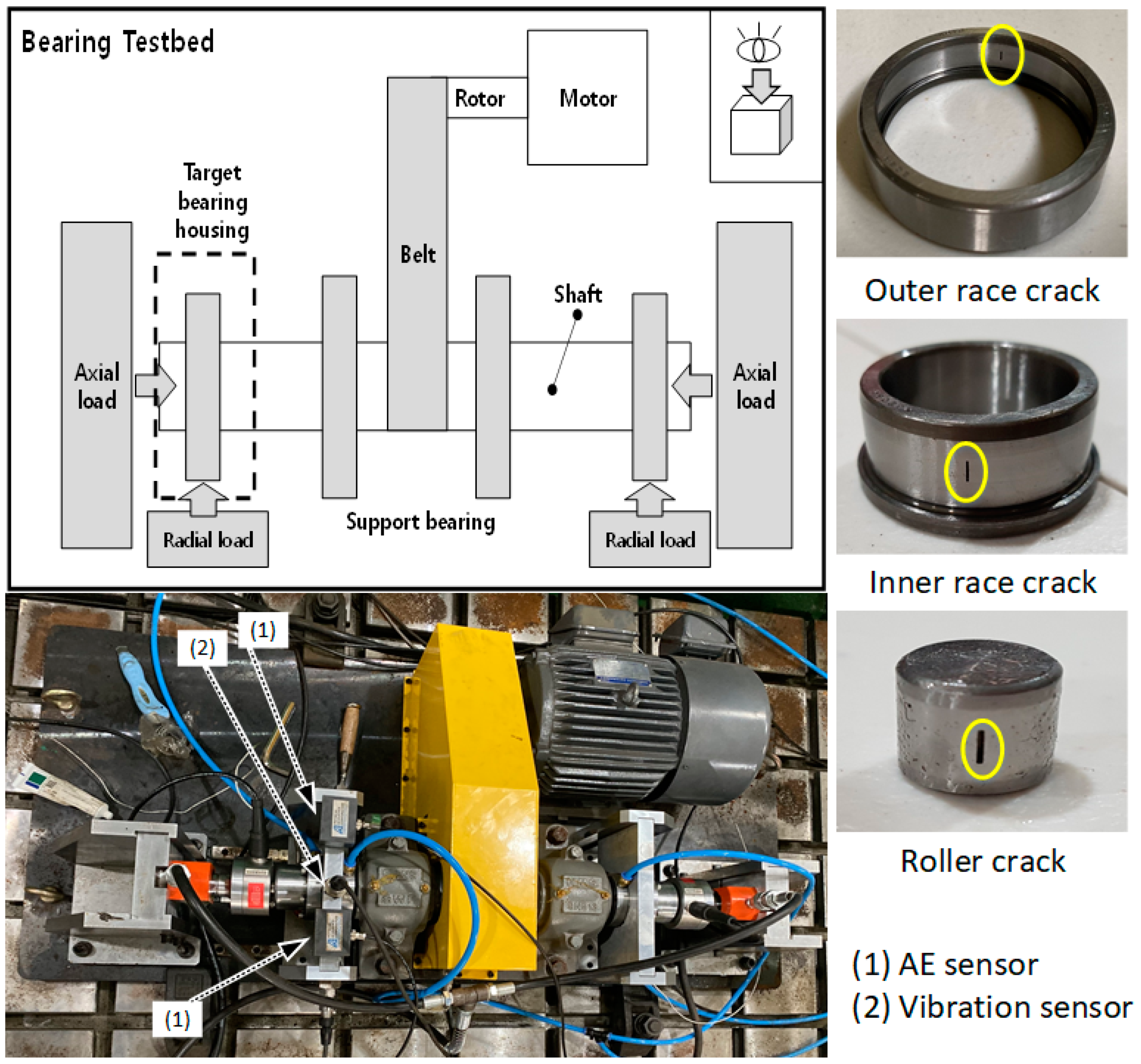
Figure 1. The self-defined testbed setup for measuring signals of bearing faults.
Applsci 10 08800 g001
Figure 2. 2-D representation of the signal corresponding to the outer fault: (a) DSWI, (b) envelope signal, (c) envelope spectrum with FO defect frequency, and (d) outer defect frequency FO, respectively.
Applsci 10 08800 g002
Figure 3. 2-D representation of the signals corresponding to the inner and roller faults: (a) DSWI for inner fault, (b) envelope signal for inner fault, (c) envelope spectrum with FI defect frequency for inner fault, (d) inner defect frequency FI, (e) DSWI for roller fault, (f) envelope signal for roller fault, (g) envelope spectrum with SF defect frequency for roller fault, and (h) roller (ball spin) defect frequency SF, respectively.
Applsci 10 08800 g003aApplsci 10 08800 g003b
Figure 4. Generating the DSWI representation and process for fault diagnosis.
Applsci 10 08800 g004
Figure 5. The proposed deep convolution neural network architecture diagram for the 128 × 128 size images.
Applsci 10 08800 g005
Figure 6. The generated image of bearing fault signal from different methods: (a) Vibration image (b) Conventional Wavelet spectrogram image (c) DSWI.
Applsci 10 08800 g006
Figure 7. The confusion matrix for the test dataset with the proposed DCNN using different types of input image: (a) Vibration image (b) Conventional Wavelet spectrogram image (c) DSWI.
Applsci 10 08800 g007
Table 1. Specifications of measuring sensors and data acquisition card.
DevicesDetailed Specification
AE sensor R15I-AST
-
Resonant frequency: 150 kHz (Ref in V/µbar)
-
Operating range: 50–400 kHz
-
Peak sensitivity: −22 dB (Ref in V/µbar)
Vibration sensor PCB-622B01
-
Frequency range: from 0.2 to 15,000 Hz
-
Measurement range: ±490 m/s2
-
Sensor sensitivity: 100 mV/g
DAQ type NI 9234
-
Operating condition: −40 °C to 70 °C operating
-
Dynamic range: 102 dB
-
Resolution: 24-bit
-
IEPE signal conditioning with AC coupling (2 mA)
Table 2. The classification report of the test dataset for different types of input and different classification methodology.
ScenariosTypeVibration Image MethodWavelet SpectrogramDSWI
(1) KNN + PCANormal35.50%0%93.50%
Outer 41.90%100%88.70%
Inner30.60%45.20%61.30%
Roller98.40%50.00%0%
Average accuracy51.42%48.99%61.13%
(2) MCSVM + PCANormal100%75.20%85.20%
Outer 96.80%84.23%90.02%
Inner91.90%86.80%86.70%
Roller35.50%81.40%89.12%
Average accuracy80.97%81.91%87.76%
(3) LeNet-5Normal32.25%96.77%93.54%
Outer 65.00%100%96.77%
Inner35.00%59.67%93.54%
Roller60.00%100%100%
Average accuracy46.77%89.11%95.97%
(4) AlexNetNormal64.52%64.51%98.38%
Outer 100%100%100%
Inner13.33%98.38%93.54%
Roller96.77%100%100%
Average accuracy68.54%90.72%97.98%
Proposed DCNNNormal100%75.80%96.80%
Outer88.70%100%100%
Inner59.70%96.80%98.40%
Roller83.90%100%100%
Average accuracy83.06%93.15%98.79%
Publisher’s Note: MDPI stays neutral with regard to jurisdictional claims in published maps and institutional affiliations.