Damage Detection Method Based on Continuous Wavelet Transformation of Lamb Wave Signals

Abstract

A damage estimation method based on continuous wavelet transformation (CWT) of the normalized Lamb wave signals is proposed here. Lamb waves are actuated and sensed using piezoelectric (lead zirconate titanate, PZT) transducers arranged in the form of square detection cells on a plate-like structure. Excitation sequences based on pitch–catch and pulse–echo configurations are tested for the same arrangement of the transducers. The possibilities of the existence of damage for each actuator–senor pair are formed by using the normalized coefficient of CWT. The size of the possible damage region is directly controlled through envelopes defined by the coefficients of CWT, and no additional parameter is required to define its size. The aggregate damage image is constructed by the fusion of damage possibilities from all actuator–sensor pairs using damage indices based on conjunctive and compromised fusion schemes. The results indicate that the proposed method can estimate the location and severity of multiple damage with signals directly from the damaged plate, without the need of baseline signals from the undamaged plate, and the time-compensated signals provide better damage imaging than the raw signals. The most accurate and computationally inexpensive combination is the pulse–echo configuration with damage index based on conjunctive image fusion scheme. The method is computationally inexpensive and can be applied for multiple damage estimations in large structures to reduce the evaluation cost and inspection time during on-line structural health monitoring.

1. Introduction

The traditional nondestructive testing (NDT) methods are useful, but they are time consuming and expensive as they require the structures to be off-service and disassembled in components. Alternatively, on-line structural health monitoring (SHM) provides a continuous assessment of structures and predicts the remaining lifespan using permanently embedded sensing systems [1]. The SHM techniques based on Lamb waves (a type of guided wave) have been extensively used for thin plate-like structures because they can travel a long distance with low attenuation, and their propagation is sensitive to the presence of small damage. The piezoelectric (lead zirconate titanate, PZT) transducers can both excite and sense the Lamb wave signals and can be permanently attached to the host structure in the form of a network of sensors for fast multipoint measurement in situ SHM [2]. These PZT transducers are small, lightweight, consume low power, and produce response in a wide frequency region [3]. Furthermore, PZT transducers can be used in harsh temperature and radiation environments for SHM of various types of damage in metallic and composite plates [4].

There are several damage estimation methods based on the sparse array of PZT transducers, which have shown a great potential for the identification of local damage. However, the Lamb wave signals generated by PZT transducers are dispersive and multimodal. An accurate interpretation of transducer data is important for the extraction of damage features such as location and severity from complicated Lamb wave signals. Therefore, sophisticated signal processing techniques such as fast Fourier transform [5], short-time Fourier transform [6], Hilbert transform [7], warped frequency transform [8], and signal-difference-based correlation coefficient [9,10] have been used to accurately analyze the dynamic response signals scattered by damage. Among these methods, the continuous wavelet transformation (CWT) [11,12] has recently gained attention and popularity due to its powerful time–frequency feature extraction from complicated signals, its ability to detect the signal singularity for physical damage inspection, and to depress the dispersive characteristics of the Lamb waves [13,14].

In recent years, Lamb-wave-based imaging methods such as phased array [15,16] and delay-and-sum [17,18,19] algorithms have been widely used for damage localization in plate-like structures. The damage imaging methods have been further empowered by probabilistic approaches such as Probability-Based Diagnostic Imaging (PDI) [20,21,22], Reconstruction Algorithm for Probabilistic Inspection of Damage (RAPID) [23,24], Algebraic Reconstruction Techniques (ART), and Lamb Wave Tomography (LWT) [25,26]. These methods have used different parameters to define the probability regions for individual sensing paths, which were then used to reconstruct the damage images. For example, the PDI methods have used the weight distribution functions [20,21,27,28,29,30] to define the probability region between actuator–sensor pairs. These distribution functions depended on a scale/shape factor, β, which controlled the effective size of the elliptical probability area for each sensing path. Similarly, the RAPID and LWT methods used the difference between damaged and undamaged signals to define the signal difference coefficient (SDC) [23,24,31,32,33,34]. The SDC also depended on β, which controlled the effective size of the probability region. In most of these methods, the probability of finding the damage depended on the intersection of direct paths between actuator–sensors pairs [20,21,23,24,25,30,33,34,35,36]. The probability of accurately locating the damage increases if more direct path intersections fall around the damage region. Consequently, the use of more transducers increases the path intersections and obtains more accurate damage imaging. That is one of the reasons why these methods faced difficulties locating the multiple damage with fewer transducers. Furthermore, these methods were based on the signal difference obtained by the comparison of the damaged signal with the baseline signal, which required additional data to be recorded and processed [27,29,30,31,33,34,35,36], and the baseline data may not always be available for practical applications.

In the current research, instead of using any probability distribution function, the possibilities of damage presence are directly defined by CWT of the normalized damage-scattered signals. No separate parameter is used to define the size of the possibility region, it is directly defined by the damage-scattered peak in the normalized CWT signals. The damage possibilities from individual sensing pairs are fused using conjunctive and compromised fusion schemes to image the damage. The method was tested for pitch–catch and pulse–echo arrangements of transducers. The damage localization was improved by a time compensation in all the original output signals. First, the single and multiple damage cases were tested using the difference signals, and then the results were obtained for the same cases directly from the damaged signals, without the baseline.

The organization of the article is as follows: Section 2 introduces the background and basic theory of the proposed method, Section 3 shows the implementation of the proposed method using difference signals, the baseline-free implementation is shown in Section 4, the influence of the environmental noise is presented in Section 5, experimental validation of the proposed method is presented in Section 6, a comprehensive discussion of results is presented in Section 7, and concluding remarks are summarized in Section 8.

2. Damage Estimation Method Based on CWT

The proposed damage estimation method describes a color-mapped image for each actuator–sensor pair, which indicates the possibility of the presence of damage in the discretized monitoring region. The region of maximum possibilities in the aggregate image of all the pairs represents the damage features. In time-of-flight (ToF)-based triangulation of a point damage $D\left(x, y\right)$, when actuator $A\left(x_i,y_i\right)$ excites the Lamb waves, sensor $S\left(x_j,y_j\right)$ receives two signals: a direct signal from $A$ to $S$, which travels a distance, $L_{A-S}$, and a damage-scattered signal, which travels a longer distance, $L_{A-D}+L_{D-S}$, as shown in Figure 1.

The ToF from $A$ to $S$ for the damaged-scattered signal, ${\mathrm{T}}_D$, can be written as,

$${\mathrm{T}}_D\left(x,y\right)= \frac{L_{A-D}+L_{D-S}}{V}$$

(1)

where, $V$ is group velocity of the incident Lamb wave and,

$$L_{A-D}= \sqrt{{\left(x-x_i\right)}^2+{\left(y-y_i\right)}^2 }; L_{D-S}=\sqrt{{\left(x-x_j\right)}^2+{\left(y-y_j\right)}^2}$$

The theoretical solution of Equation (1) represents an elliptical path locus with focal points at $A$ and $S$, indicating the possible damage locations on it, as shown in Figure 1. When transducers are arranged as an active sensor network, the actual damage location falls at the intersection of multiple elliptical path loci from different actuator–sensor pairs. For damage localization using Equation (1), the accurate extraction of ToF is important therefore, the CWT is introduced to process the signals due to its high time–frequency resolution.

2.1. Normalized Coefficient of CWT

The coefficient of CWT for square-integrable function $f\left(t\right)$ in the time domain can be written as,

$$CW{T}_f\left(a,b\right)= \frac{1}{\sqrt{a}}{{\displaystyle \int }}_{-\infty }^{+\infty }f\left(t\right)\overline{\psi }\left(\frac{t-b}{a}\right)\mathrm{d}t,$$

(2)

where $a>0$ and $b\in ℝ$ are scale and time-shift parameters of wavelet function $\psi \left(t\right)$, respectively. During the transform, a dynamic signal is represented using these dual parameters. In this research, the scale is set as the ratio between sampling frequency and central frequency as

$$a= \frac{F_s}{F_c}$$

(3)

where $F_s$ is the sampling frequency calculated using the sampling period as $F_s=1/\Delta$, and $F_c$ is the central frequency of the excitation signal. The bar accent represents complex conjugate of the wavelet function$\psi \left(t\right)$. The selection of the mother wavelet function $\psi \left(t\right)$ is crucial for CWT applications. The Gabor wavelet function was chosen in this research for its higher time resolution to capture the ToF accurately. It has an accurate time–frequency feature extraction capability in ToF-based damage localization problems [11]. The Gabor wavelet function can be expressed as

$${\psi }_G\left(t\right)= \frac{1}{\sqrt[4]{\pi }}\sqrt{\frac{{\omega }_0}{\gamma }}\exp \left[-\frac{{\left({\omega }_0/\gamma \right)}^2}{2}{t}^2\right]\exp \left(i{\omega }_{0}t\right),$$

(4)

where ${\omega }_0$ and $\gamma$ are the real constants. ${\omega }_0=2\pi$, so that the value $1/a$ becomes equal to frequency $f= \omega /2\pi$, and $\gamma =\pi \sqrt{2/\ln 2}$ was set to satisfy the following admissibility condition:

$${{\displaystyle \int }}_{-\infty }^{\infty }{\left|\psi \left(\omega \right)\right|}^2/\omega \mathrm{d}\omega <\infty .$$

(5)

For the monitoring region discretized into a number of grid points, the possibility of damage existence at each grid point is directly defined by the coefficient of CWT for each actuator–sensor pair. The application of the coefficient of CWT, based on the Gabor wavelet, on damage-scattered signals constructs a CWT envelope for each pair. The possibilities of damage existence are expressed within the range from 0 to 1 with the maximum possibility at a grid point with value 1. Therefore, all damage-scattered signals, $f_D\left(t\right),$ were normalized by dividing with the maximum absolute value of amplitude of the corresponding signal as,

$$\widehat{f_D\left(t\right)}=\frac{f_D\left(t\right)}{\max \left(\mathrm{abs}\left(f_D\left(t\right)\right)\right)}$$

(6)

The Gabor wavelet coefficient modulus of the normalized damaged-scattered signal then extracts the damage information for further processing of damage image. It is performed as

$$I\left(b\right)=\mathrm{abs}\left(CW{T}_{\widehat{f_D\left(t\right)}}\left(a,b\right)\right)$$

(7)

2.2. Time Compensation

The value of ${\mathrm{T}}_D$ in Equation (1) represents the total ToF of excitation signal from actuator to damage and then from damage to sensor. This is the time in the dynamic response signal when the sensor starts receiving the damage-scattered signal [21]. Consider a normalized damage-scattered signal presented in Figure 2 as an example, the traveling time from actuator to sensor, ${\mathrm{T}}_D,$should be from the beginning to the point when damage-scattered signal starts to become non-zero as shown in Figure 2a. However, this non-zero point is very difficult to identify in practice. The envelope of the coefficient of CWT of this signal, based on Equation (7), is presented with red line in Figure 2b. The excitation signal used throughout this research was a 5.5-cycle sinusoidal tone burst modulated by Hann window at central frequency 383 kHz, as shown in Figure 3. For the central frequency of 383 kHz and sampling time of 0.02 $\mathsf{\mu }\mathrm{s}$, the scale parameter $a$ was calculated as 130.5 using Equation (3). If ${\mathrm{T}}_{\mathrm{e}}$ is the total acting time of the excitation signal as shown in Figure 3a, a good time–frequency analysis feature of the CWT can depress the dispersion of Lamb wave effectively to make the signal contain the same duration of time during wave propagation.

The maximum value 1 in the CWT envelope in Figure 2b appears at the center of the normalized damage-scattered peak, which is half of the time ${\mathrm{T}}_{\mathrm{e}}$ ahead of the time ${\mathrm{T}}_D$ when sensor actually received the non-zero point of the damage-scattered signal. Therefore, a time lag was introduced in all the CWT signals by subtracting ${\mathrm{T}}_{\mathrm{e}}/2$ as time-compensation ${\mathrm{T}}_{\mathrm{c}}$, shown with blue line in Figure 2b. If $N$ is the total number of cycles and $f_e$ is the central frequency of the excitation signal, ${\mathrm{T}}_{\mathrm{c}}$ can be expressed as

$${\mathrm{T}}_{\mathrm{c}}=\frac{N}{2f_e}.$$

(8)

2.3. Imaging Algorithm

The monitoring region containing the actuator–sensor pairs is divided into a uniform mesh of $N\times N$ grid points. The possibility of damage existence at a grid point $\left(x_i,y_i\right)$ for an actuator–sensor pair is represented by the damage index for a sensing pair ($DIS{P}_P\left(x_i,y_i\right)$) where, $i=1,\dots ,N$, $P=1,\dots ,N_P,$ and $N_P$ is the total number of actuator–sensor paths. The solution of Equation (1) on the mesh grid for any actuator–sensor pair provides an image with an infinite number of path loci. The grid points that have the same value of ${\mathrm{T}}_D$ fall on one path locus. The time-compensated CWT envelope of the normalized damage-scattered signal $f_D\left(t\right)$ defined by Equation (7) provides $DIS{P}_P\left(x_i,y_i\right)$) at different time values, ${\mathrm{T}}_D$. The value of $DIS{P}_P\left(x_i,y_i\right)$ can be expressed as

$$DIS{P}_P\left(x_i,y_i\right)={\left|I\left({\mathrm{T}}_D\left(x_i,y_i\right)\right)\right|}_P$$

(9)

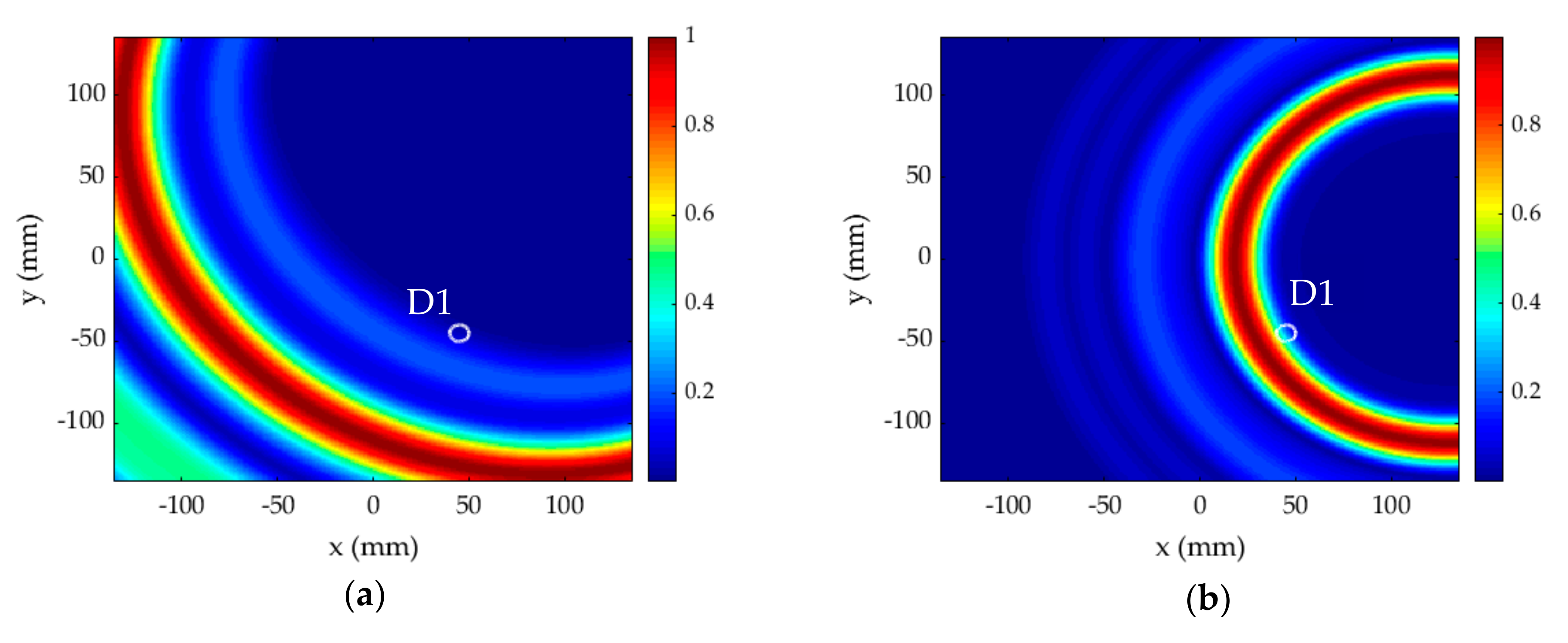
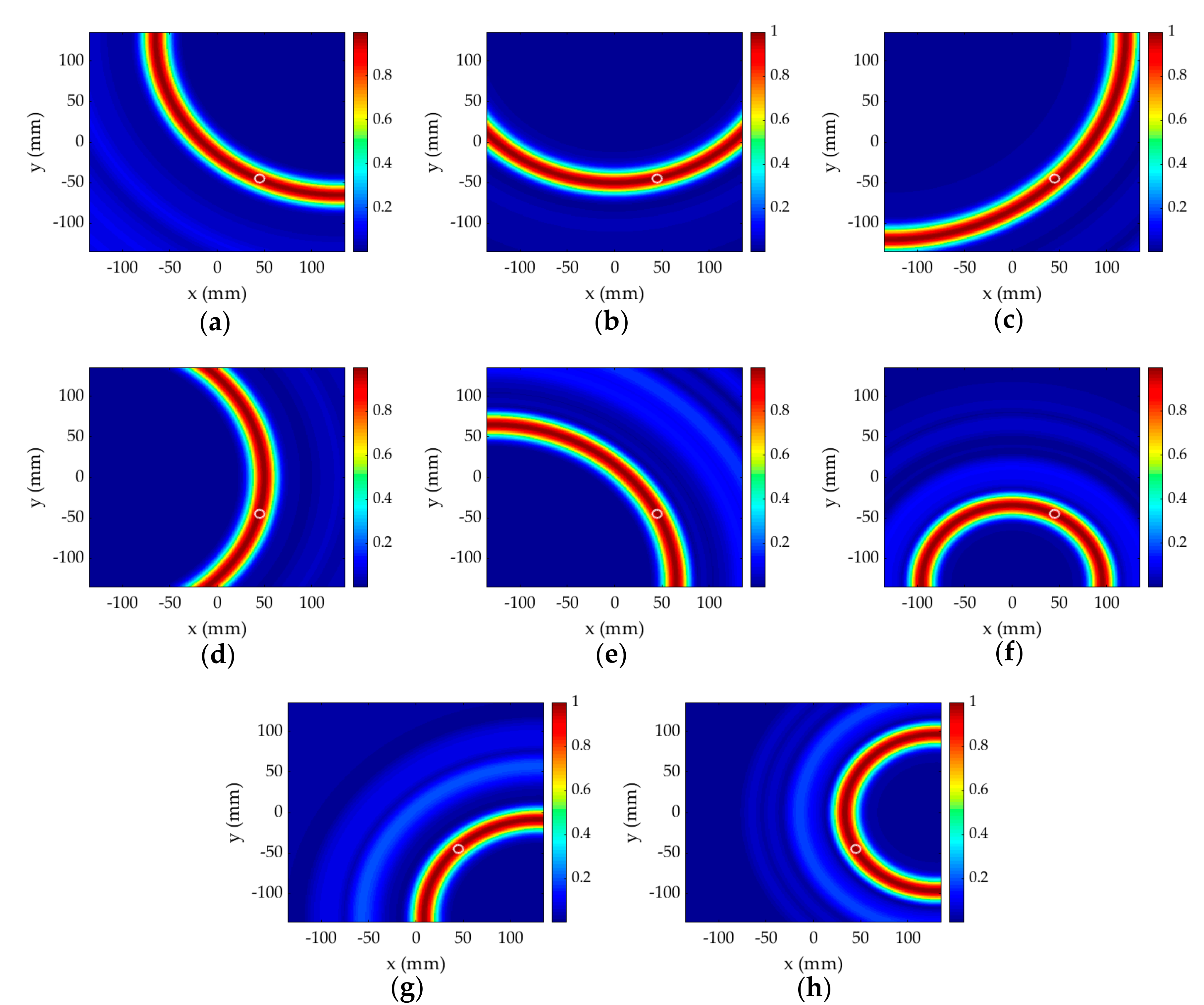
The image defined by $DIS{P}_P\left(x_i,y_i\right)$ provides possible damage locations with the maximum possibility of damage existence at the time when the peak value 1 appears in the CWT envelope. An imaging algorithm was designed in MATLAB to implement Equation (9) in three steps: In the first step, the envelopes provided by the time-compensated coefficient of CWT of the normalized damage-scattered signals were plotted based on Equation (7). In the second step, the infinite number of elliptical path loci provided by Equation (1) were plotted on the discretized domain, which provided a color-mapped image for each sensing pair. Since, Equation (1) represents the ToF of the damage-scattered signals, in step 3, the field values plotted in step 2 were replaced by the values from the CWT envelopes at the corresponding times. The image obtained in step 3 represented possible damage locations in the discretized domain for individual sensing pairs, with the maximum possibility corresponding to the same time and location as in CWT envelopes.

A damage index, $DI\left(x_i,y_i\right),$ then defines the aggregate image by fusion of $DIS{P}_P\left(x_i,y_i\right)$ images for each actuator–sensor pair. Two different image fusion schemes were tested for the proposed method: conjunctive fusion scheme based on the multiplication of $DIS{P}_P\left(x_i,y_i\right)$ values from all pairs at a grid point and compromised fusion scheme based on addition of the values. The damage indices for compromised fusion $D{I}_a\left(x_i,y_i\right)$ and conjunctive fusion $D{I}_m\left(x_i,y_i\right)$ schemes can be written as

$$D{I}_a\left(x_i,y_i\right)=\frac{1}{N_P}{\displaystyle \sum }_{P=1}^{N_P}DIS{P}_P\left(x_i,y_i\right)$$

(10)

$$D{I}_m\left(x_i,y_i\right)={\displaystyle \prod }_{P=1}^{N_P}DIS{P}_P\left(x_i,y_i\right)$$

(11)

3. Implementation Using the Difference Signals

3.1. Finite Element Simulation Model

Consider a 1000 × 1000 × 1.5 mm³ aluminum plate with PZT transducers arranged in the form of two square cells of 250 × 250 mm² and 270 × 270 mm², as shown in Figure 4. Numerical simulations were performed using a commercial finite element software, ABAQUS Explicit, and the material properties were $\mathrm{E}=71 \mathrm{GP}$a, $\mathsf{\upsilon }$ = 0.3, and $\mathsf{\rho }$ = 2700 ${\mathrm{kg}/\mathrm{m}}^3$. Each PZT transducer had a diameter of 5 mm, and it could excite or sense the Lamb wave signals in radially outward directions. In order to excite the Lamb wave signals, a uniformly distributed load was applied in cylindrical coordinates with amplitude as the excitation frequency, as shown at point A in Figure 1.

A circular damage of 10 mm diameter was made as a through-hole located at (45, −45) mm from center of the plate. The plate was meshed with 3D shell elements S4R with the element size of 1 mm in all simulation models, and a time step of $0.02 \mathsf{\mu }\mathrm{s}$ was used to accurately simulate the Lamb wave propagation for a total time of 150$\mathsf{\mu }\mathrm{s}$.

3.2. Dispersion Curves

The dispersion curves were drawn for Lamb wave propagation in aluminum plate, which had both symmetric (S) and anti-symmetric (A) modes propagating simultaneously, as shown in Figure 5.

In the low-frequency range, only S₀ and A₀ modes propagated, with the group velocity of S₀ mode significantly higher than that of the A₀ mode. If a modified signal with narrow frequency band is excited, both the modes can be identified separately, with the peak of S₀ arriving first. In case of mode conversion after scattering from damage, S₀ will still reflect a faster symmetric mode S₀ and a slower anti-symmetric mode A₀. Therefore, the scattered S₀ mode is also easy to identify as one propagating faster, and it was exclusively chosen in the method proposed here.

The frequency–thickness product ($f\times d$) was calculated as 574.5 Hz⋅m for the excitation frequency of 383 kHz and plate thickness of 1.5 mm. This point existed in the low-frequency range of the dispersion curves, where the S₀ mode could be easily separated from the A₀ mode, as shown with the vertical red dashed line in Figure 5. The simulation model was validated first by calculating the group velocity, $V$, in Equation (1). The group velocity calculated through simulations was $5.31 \times 103$ m/s, which was almost the same as obtained from the dispersion curves. It indicates that the simulation model had good accuracy to calculate the Lamb wave propagation.

3.3. Excitation Configurations

Two different excitation sequences were chosen to test the proposed method in pitch–catch and pulse–echo configurations. In the pitch–catch configuration, all the A points in Figure 4 excited the Lamb wave signals one by one, and other A points acted as receivers with total of 28 actuator–sensor pairs, i.e., $\mathrm{A}i\mathrm{A}j$, $i = 1,\dots ,8$, $j = 1,\dots ,8$, $i\ne j$. This configuration ensured that damage existed in the region between the actuator and sensor for each pair. In the pulse–echo configuration, all the A points excited the Lamb wave signals, and the corresponding B points acted as receivers, i.e., $\mathrm{A}i\mathrm{B}i$, $i = 1,\dots ,8$, with total of 8 actuator–sensor pairs. The actuator and sensor existed close to each other on one side and damage on the other side in this configuration. The monitoring region containing the actuator–sensor pairs was divided into a uniform mesh of $400\times 400$ grid points with spacing of 1 mm between the neighboring points. The solution of Equation (1) on the mesh grid for any actuator–sensor pair without the damage provided an infinite number of path loci. When actuator and sensor were far from each other in the pitch–catch configuration, the path loci were ellipse-like, as shown in Figure 6a for pair A2A8. When actuator and sensor were close to each other in the pulse–echo configuration, the path loci were circle-like, as shown in Figure 6b for pair A8B8.

3.4. Single Damage Scenario

For the single damage scenario shown in Figure 4, if the pitch–catch configuration was utilized, the signals from A2 to A8 in undamaged and damaged plates are shown in Figure 7a,b, respectively. The undamaged signal contained the excitation signal S₀, which travelled a direct path between actuator to sensor represented by distance $L_{A-s}$ in Figure 1, and another signal scattered by edge of the plate. The damaged signal contained the direct excitation S₀ and a damage-scattered signal, which travelled a longer distance $L_{A-D}+L_{D-S}$. The undamaged and damaged dynamic response signals were evaluated in the discrete form in the time domain. The subtraction of the undamaged signal from the damaged signal was called the difference signal, which represented the presence of damage in the plate. The difference of the signals in Figure 7a,b is presented in Figure 7c. The first fluctuation in the difference signal represented the damage-scattered signal whereas, rest of the scatterings in Figure 7b,c were caused by the plate edges. The ToF for damage-scattered signals in Figure 7b,c was represented by Equation (1). The coefficient of CWT for the normalized difference signal was calculated using Equation (7), which provided the possibilities envelope for damage imaging, presented in Figure 7d. Similarly, the damage possibilities curves for all other actuator–sensor pairs in pitch–catch configuration were calculated.

In the pulse–echo configuration, when A8 excited the Lamb wave signal and B8 received the signal, the undamaged and damaged signals are presented in Figure 8a,b, respectively. The first fluctuation in the difference signal presented in Figure 8c was caused by the scattering from the damage, and the remaining fluctuations were caused by the scattering from plate edges. The coefficient of the normalized CWT signal as the damage possibilities curve for A8S8 is presented in Figure 8d. Similarly, the damage possibility envelopes for all other actuator–sensor pairs were calculated for the pulse–echo configuration. The envelopes based on the peaks of CWT coefficients in Figure 7d and Figure 8d defined the possibilities of damage existence as a field value for the set of path loci shown in Figure 6a,b, respectively, using Equation (9).

The time compensation in CWT signals was not made at this stage. The resulting damage possibility images for paths A2A8 and A8B8 are shown in Figure 9a,b, respectively. The actual damage D1 is also presented in these figures, which falls on the first fluctuation in the difference signal, as explained earlier. Similar damage possibility images were created for each sensing path in both the configurations. For the pitch–catch configuration, $D{I}_a\left(x_i,y_i\right)$ based on the compromised fusion scheme and $D{I}_m\left(x_i,y_i\right)$ based on the conjunctive fusion scheme provided the aggregate possibility for damage estimation in Figure 10a,b, respectively. Similarly, for the pulse–echo configuration, the aggregate damage images for $D{I}_a\left(x_i,y_i\right)$ and $D{I}_m\left(x_i,y_i\right)$ are shown in Figure 11a,b, respectively. The results indicate that the pulse–echo configuration provided a better damage estimation in both the fusion schemes with only eight sensing paths as compared to the pitch–catch configuration with 28 sensing paths. Therefore, the pulse–echo configuration was used for the remaining analyses in this paper.

3.5. Effect of Time Compensation

The possibilities of damage existence for all eight sensing paths A1B1 to A8B8 in pulse–echo configuration are presented in Figure 12a–h, respectively. These plots were based on the normalized CWT signals without the time compensation, and it can be noticed that the maximum possibility regions are ahead in time with respect to the actual damage position. The time compensation in all the CWT signals was made based on the discussion in Section 2.2. As an example, the signals for sensing pair A8B8 are presented again in Figure 13. The undamaged, damaged, and difference signals are presented in Figure 13a–c, respectively. The envelopes of normalized coefficient of CWT with time compensation (blue) and without time compensation (red) are presented in Figure 13d.

The damage possibilities for sensing paths A1B1 to A8B8 are presented again with time-compensated signals in Figure 14a–h, respectively. It can be seen that the maximum possibility regions coincide with the actual damage locations in this case. The aggregate damage images for $D{I}_a\left(x_i,y_i\right)$ and $D{I}_m\left(x_i,y_i\right)$ using the time-compensated signals are shown in Figure 15a,b, respectively. The results indicate that the time-compensated signals could localize the damage accurately for both the fusion schemes. However, the damage index based on the conjunctive fusion scheme can provide better damage imaging than that on compromised fusion scheme. Therefore, the pulse–echo configuration with damage index based on conjunctive fusion scheme $D{I}_m\left(x_i,y_i\right)$ is proposed in this method, and this combination was chosen for the remaining analyses in this paper.

3.6. Multiple Damage Scenario

To test the method for the multiple damage scenario, an additional damage D2 of 12 mm diameter was formed as a through-hole in the model shown in Figure 4. The damage D2 was located at (−30, 50) mm from center of the plate, as shown in Figure 16.

The dynamic response signals for sensing path A8B8 are presented again in Figure 17 for the multiple damage scenario. The undamaged signal shown in Figure 17a only contained the direct excitation signal S₀, whereas the damaged signal shown in Figure 17b contained two additional damage-scattered signals. The damage-scattered peaks are more prominent in the difference signal shown in Figure 17c. The CWT envelopes of difference signal with and without time compensation are shown in Figure 17d. The damage possibilities for sensing path A8B8 are presented in Figure 18 along with the actual size and location of damage D1 and D2. The possibilities of damage existence without time compensation are presented in Figure 18a and with time-compensation in Figure 18b. Similarly, the possibilities from the other seven sensing paths were plotted and fused for damage imaging.

The aggregate images based on damage index, $D{I}_m\left(x_i,y_i\right),$ without time compensation and with time compensation are shown in Figure 19a,b, respectively. The results show the importance of time compensation. The time-compensated signals could accurately image both the damage, whereas the localization of damage without compensation was inaccurate.

4. Implementation Using the Damaged Signals

The baseline signals from the undamaged plate may not always be available to calculate the difference signals in the practical environment. It also increases the computational cost by calculating two additional signals for each sensing path, i.e., undamaged and difference signals. In addition, a tiny incorrect baseline can make the whole estimation wrong. Therefore, the proposed method was implemented using signals directly from the current state of the plate. 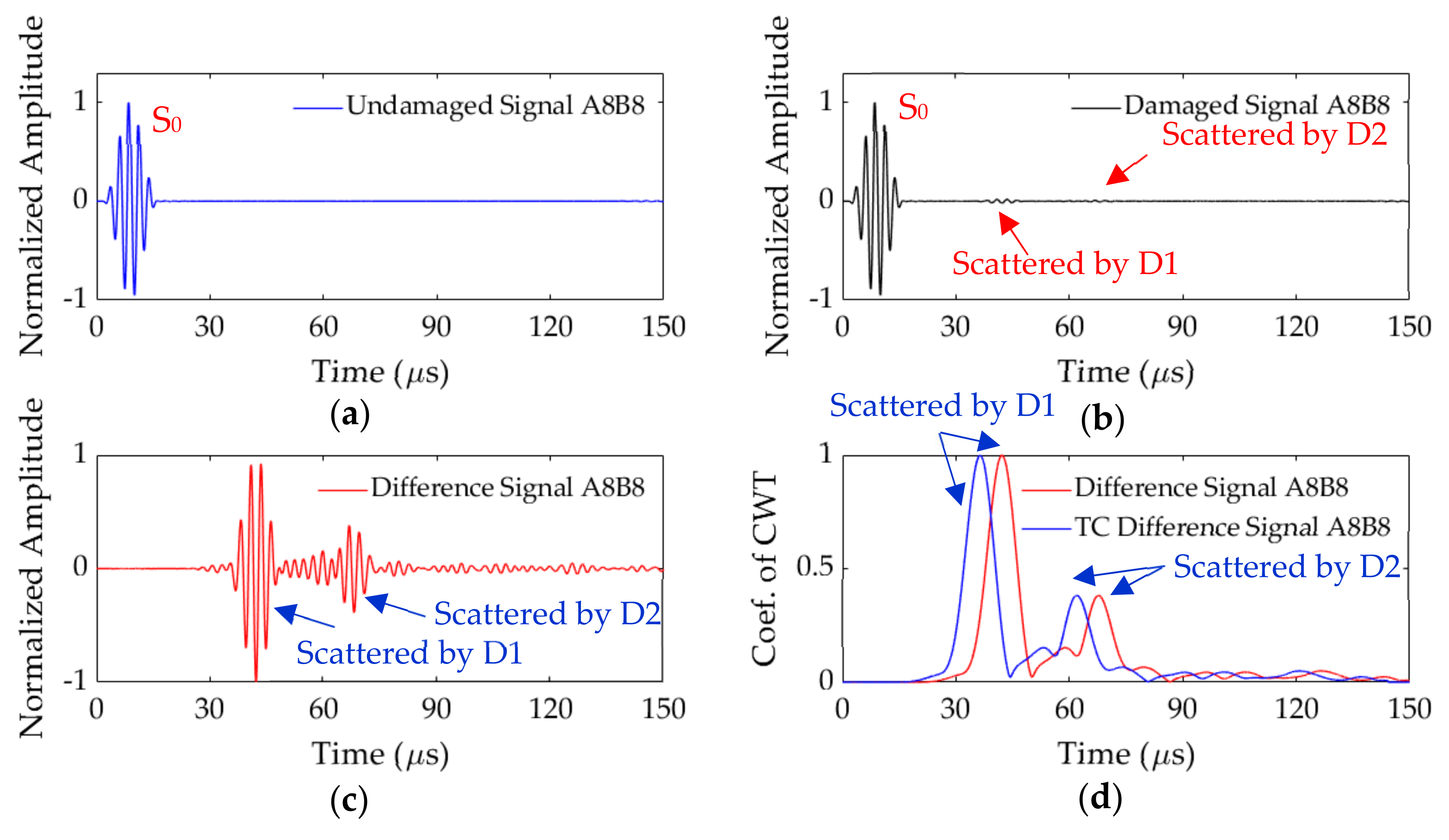The baseline-free implementation presented here is for the multiple damage scenario shown in Figure 16. The damaged signal and coefficient of CWT for sensing path A8B8 are shown in Figure 20a,b, respectively. The damage-scattered fluctuations in these signals are too small compared to the excitation fluctuation; therefore, the region of these plots containing the damage-scattered fluctuations is shown separately in Figure 20c,d, respectively. The damage-scattered peaks can be clearly seen in Figure 20d.

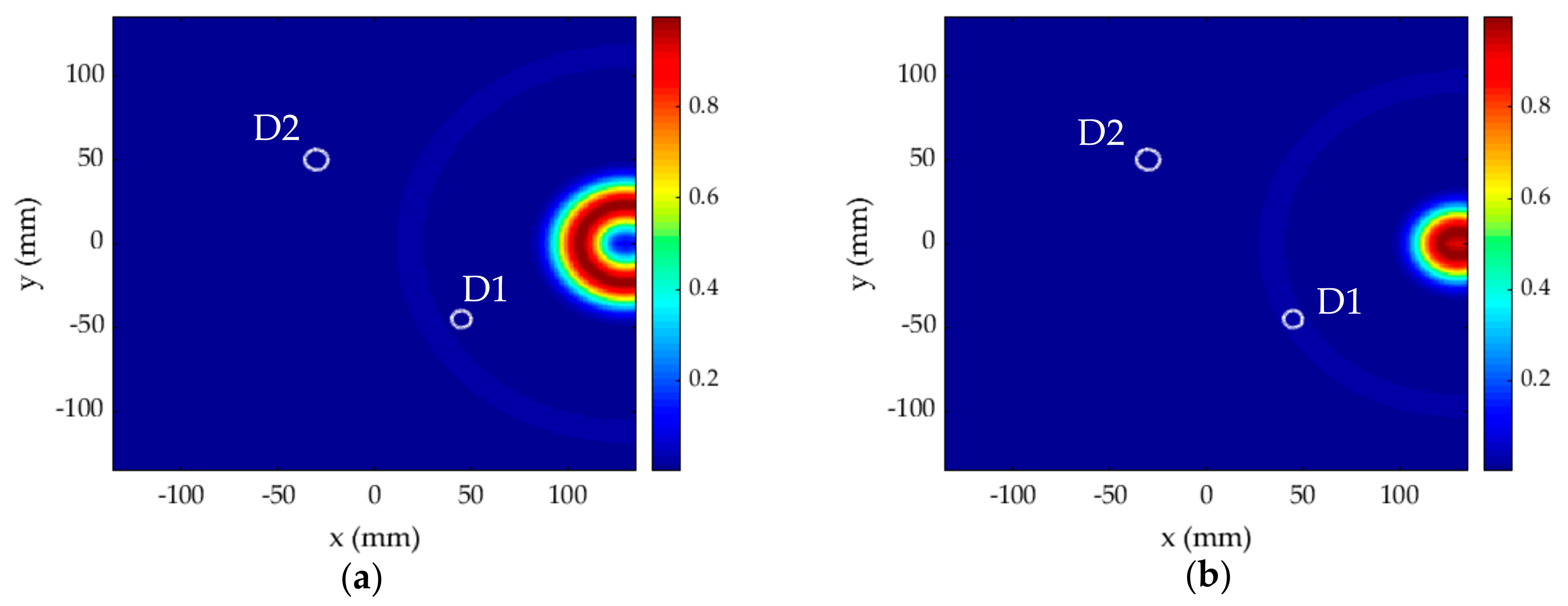
The damage possibilities for sensing path A8B8 using baseline-free estimations are presented in Figure 21 along with actual D1 and D2. Figure 21a contains the possibilities without time compensation and Figure 21b with time compensation. Since, the damage-scattered peaks are too small, the damage possibility values for D1 is hardly visible, whereas for D2 it is so small that it is not even visible. It is because the possibility values for the excitation peak is very high. Similar to Figure 20c,d, the damage-focused regions of Figure 21a,b are shown separately in Figure 22a,b, respectively. The highest damage possibility region near the actuator–sensor locations has been left out of these images, and the distributions around D1 and D2 are more visible now compared to surrounding regions.

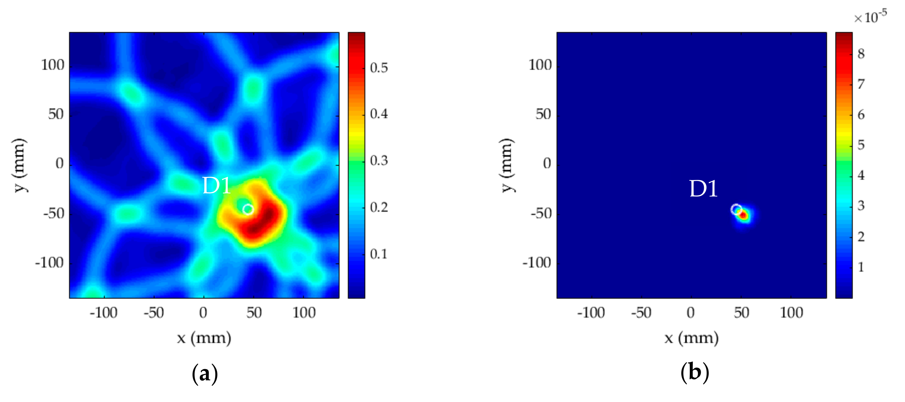
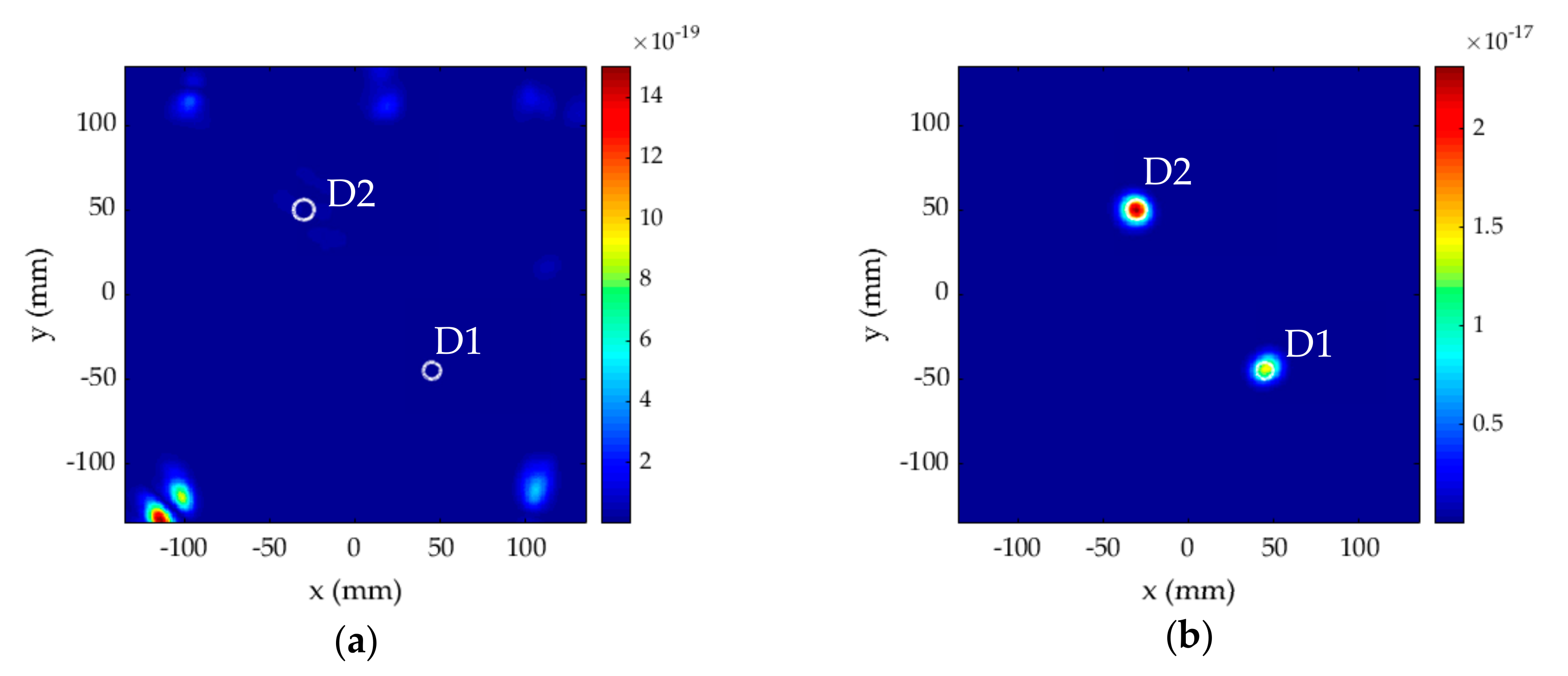
Similarly, the damage possibilities from the other seven sensing paths were plotted and fused for damage imaging. The high-possibility regions for each sensing pair were near the actuator–sensor pairs, just as for the case of A8B8. The aggregate images without and with time compensation are shown in Figure 23a,b, respectively. The time-compensated signals could accurately image both the damage, whereas the localization of damage without compensation did not work for this case either. It should be noticed that the high-possibility regions near each actuator–sensor pair disappeared in the aggregate image. It is because the possibility values from other sensing pairs at these locations were almost 0, which reduced the aggregate value to 0 using multiplication-based $D{I}_m\left(x_i,y_i\right)$. The individual damage possibility values from all 8 sensing pairs and the aggregate value at damage locations based on $D{I}_m\left(x_i,y_i\right)$ are presented in

Table 1. Possibilities of damage existence values at damage locations from all sensing pairs in pulse–echo configuration.

Pair Location (mm)	A1B1	A2B2	A3B3	A4B4	A5B5	A6B6	A7B7	A8B8	$\mathit{D}{\mathit{I}}_{\mathit{m}}\left({\mathit{x}}_{\mathit{i}},{\mathit{y}}_{\mathit{i}}\right)$
D1 (45, −45)	0.0073	0.0060	0.0032	0.0070	0.0024	0.0191	0.0155	0.0201	1.41 × 10−17
D2 (−30, 50)	0.0047	0.0325	0.0172	0.0205	0.0047	0.0064	0.0019	0.0073	2.30 × 10−17

for the pulse–echo configuration. Non-zero damage possibility values from all sensing pairs existed at the damage locations, which made the non-zero aggregate value appear only at the damage locations.

5. Influence of Environmental Noise

It is essential to test the noise tolerance of the proposed method for the real-world signals, which may be noisy and can influence the results when damage-scattered peaks are too small. The white noise signals in Gaussian distribution were artificially added to the original damaged signals. A high value of noise, i.e., signal-to-noise ratio (SNR) of 30 dB, was added to all the damaged signals, and envelopes formed by the coefficient of CWT were reevaluated. The signals shown in Figure 20a,b are presented again with SNR 30 dB in Figure 24a,b, respectively. A high influence of the noise in the signals can be observed in damaged-focused region of these plots separately shown in Figure 24c,d, respectively.

The possibilities for damage existence for all sensing paths in the pulse–echo configuration were evaluated with noisy signals and then fused to get the aggregate damage image. The results for multiple damage scenario with noisy baseline-free signals are shown in Figure 25a,b, respectively, without and with the time compensation. Although the noise has a little influence on the resolution of damage imaging, the proposed method could still accurately locate both the damage, and also estimate the severity of one damage with respect to the other damage.

6. Experimental Evaluation

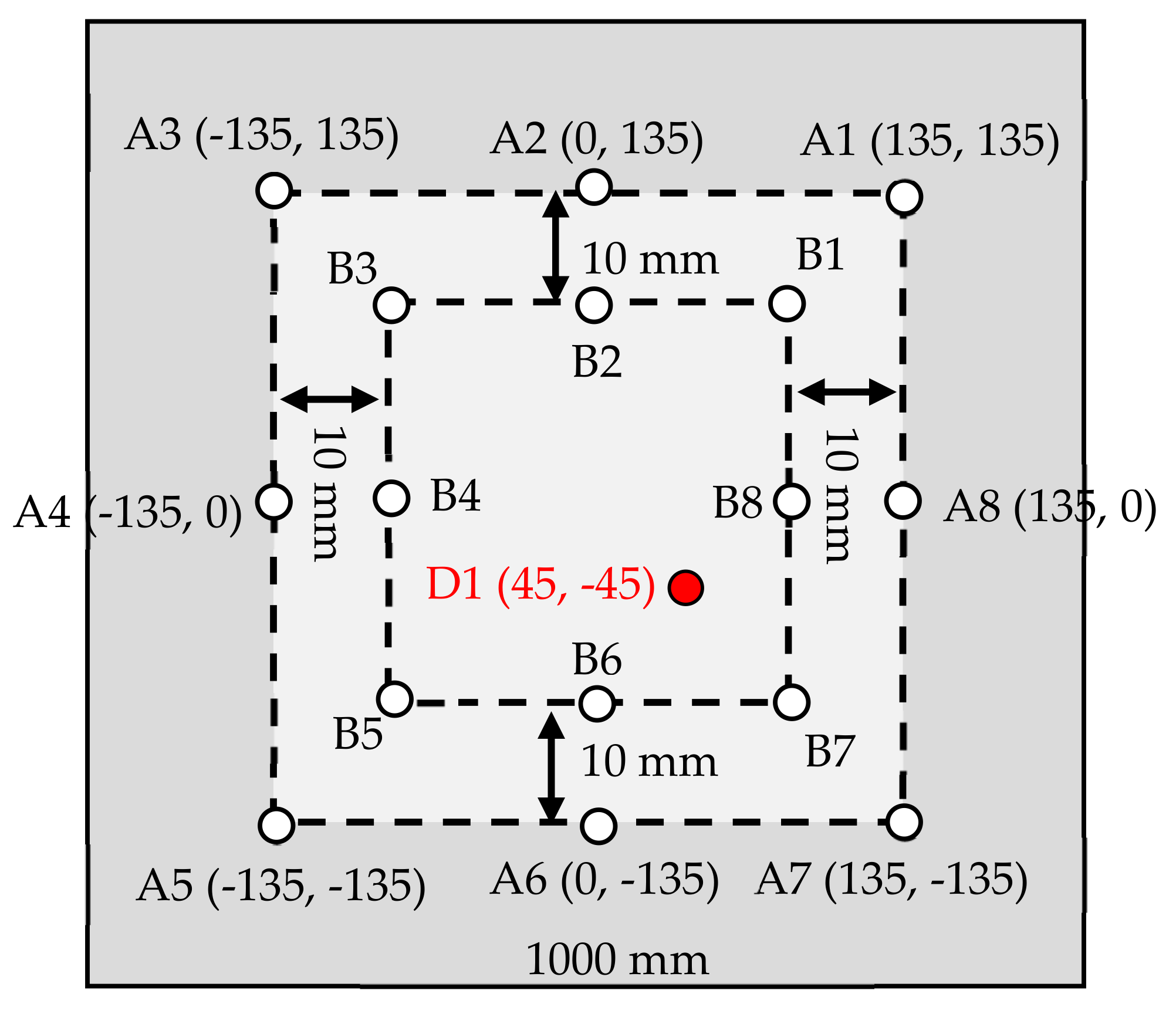
The accuracy of the proposed method was further tested through experimental investigation performed on an 800 × 800 × 1.5 mm³ aluminum plate with PZT wafers arranged in the form of two square cells of 300 × 300 mm² and 240 × 240 mm², as shown in Figure 26a. The minimum size of the damage that can be estimated using the Lamb wave should be equal to or greater than half of its wavelength. For 383 kHz frequency excitation and $5.31 \times 103$ m/s group velocity, the wavelength was about 14 mm, therefore, a damage was formed as a punch hole of 7 mm diameter located at (−90, 30) mm. The size of each PZT wafer used in experiments was 5.4 mm diameter, and they were made up of PSN-33 with a density of 7.70 × 10³ kg/m³. The PZT wafers had a resonance frequency of 383 kHz, and they could excite/sense the Lamb wave signals in radially outward directions. The real-time laboratory setup of the experiment is shown in Figure 26b. The signal generator (RIGOL, DG1022) was programmed to generate the excitation signal shown in Figure 3a. The signal was amplified to 4.2 V using a power amplifier (KROHN-HITE, 7602M). The dynamic response signals were recorded at each receiving transducer using a four-channel oscilloscope (LeCroy, LC574AL). The response signals were captured over a sampling time of 200 $\mathsf{\mu }\mathrm{s}$ at the sampling rate of 1 GHz. In order to reduce the noise, each signal was acquired for an average of 500 times.

When A1 excited the Lamb wave signal, the damaged signal recorded at B1 is presented in Figure 27a, which contains three fluctuations: excitation, damage-scattered, and edge-scattered. Similarly, when A2 was excited, the recorded signal at B2 is presented in Figure 27b, which contains two fluctuations: one is excitation fluctuation and another is damage-scattered overlapped with edge-scattered. The envelopes of the coefficient of CWT for signals at A1B1 and A2B2 are presented in Figure 27c,d, respectively. The time compensation was already made in the experimental signals during the data recording as the oscilloscope was set to trigger or start recording when peak of the voltage signal appears. The damage possibilities for sensing paths A1B1 and A2B2 are presented in Figure 28a,b, respectively, along with actual size and location of damage D3. The damage-scattered fluctuation in Figure 28b is overlapped with edge-scattered fluctuation, therefore it does not represent the correct possibilities of damage existence. In the current experimental evaluation, the baseline signals from the undamaged plate were not utilized, therefore the damage possibilities from sensing pair A2B2 were not used in the aggregate damage imaging. Similarly, the damage possibilities for all useful sensing paths in the pulse–echo configuration were evaluated and fused to get the aggregate damage image, presented in Figure 29.

The results validate that the proposed method can locate the damage with relatively good accuracy also through experimental data. The method proposes the arrangement of PZT transducers as a network of square detection cells on a large structure. Since, the wave velocity and location of the plate edges are already known, the total time for wave propagation can be calculated accordingly to avoid the edge scatterings for all the central cells. For detection cells near the physical boundary, there may be both the damage-scattered and edge-scattered fluctuations, which can be identified separately as shown in Figure 27a for sensing pair A1B1.

In a rare case, when distances between damage location and receiver and plate’s edge and receiver are same for one of the sensing pairs, the damage-scattered and edge-scattered fluctuation may overlap, as shown in Figure 27b for sensing pair A2B2. The possibilities of damage existence from such sensing paths where the damage scatterings are weak and overlapped with incident waves or edge scatterings can be ignored in the aggregate damage imaging. Alternatively, the baseline can be used for cells near the physical boundary of the plate in practical applications.

7. Discussion of Results

Two different excitation configurations, pitch–catch and pulse–echo, and damage index based on two different image fusion schemes, compromised fusion $D{I}_a\left(x_i,y_i\right)$ and conjunctive fusion $D{I}_m\left(x_i,y_i\right)$, were tested in the proposed method. The results presented in Figure 10 and Figure 11 verified that the pulse–echo configuration with the conjunctive fusion scheme was most suitable for the proposed method. The pulse–echo configuration was also computationally inexpensive as it provided better accuracy with only 8 excitations compared to the pitch–catch configuration with 28 excitations.

The comparison of signals presented for pulse–echo configuration in Figure 8, Figure 13, Figure 17, and Figure 20 with pitch–catch configuration signals presented in Figure 7 showed that the damage scatterings were much stronger than the edge scatterings in case of pulse–echo configuration, whereas the edge scatterings were stronger in case of pitch–catch configuration, for the same size of damage in both cases. This made the high-possibilities region appear at the edge location instead of the damage location during pitch–catch estimation, as shown in Figure 9a. This is one of the reasons why inaccuracies appeared in damage estimation based on the pitch–catch configuration.

The damage possibilities envelopes defined by the coefficient of CWT were normalized in order to range the possibility values from minimum 0 to maximum 1. The damage index $D{I}_m\left(x_i,y_i\right)$ produced better estimation of the damage region because it is based on the multiplication of the possibility values at grid points from each sensing path. When the damage possibilities for an individual path were too high at a non-damaged location, it still reduced to zero in the aggregate image when multiplied with the values from other sensing paths at the same region. The non-zero values of possibility in the aggregate image appeared only at the damage location because the values from all sensing paths were non-zero at that location. For the same reason, $D{I}_m\left(x_i,y_i\right)$ worked well even when the damage-scattered fluctuations were too small compared to the excitation fluctuation S₀ for baseline-free signals in Figure 20. Although, the damage-scattered peaks and damage possibilities were too small for an individual sensing path, all the higher-value regions disappeared in the aggregate image because values from other paths at those locations were 0, leaving behind only the damage region having a non-zero contribution from all sensing paths, as evident from Figure 23b.

The results presented in Figure 19b and Figure 23b indicated that multiple damage could be accurately estimated with and without the baseline signals. The method could not only accurately locate the damage but also provided the severity of each damage with respect to the other. In these imaging results, the damage D2 of 12 mm diameter appeared to have a higher possibility values than the smaller damage D1 of 10 mm diameter. It made the damage image for D2 more severe in intensity and extent than that of D1.

The damage index was based on CWT signals, which have a better signal-to-noise ratio and can extract the time–frequency characteristics exactly from the noisy real-world signals. That is why CWT could process the Lamb signals directly from the damaged plate without a baseline signal from an undamaged plate. In the proposed pulse–echo configuration, the damage-scattered peaks in CWT envelopes were much more dominant than other peaks, therefore any additional noise in real-world problems would still ensure that the damage-scattered peaks have the maximum value of 1 in the CWT envelopes for accurate damage estimation.

Generally, the Lamb waves are dispersive in nature, which causes an error in determining its characteristics. The time compensation equal to the half period of the excitation signal is valid when the Lamb waves are not dispersive. In case of a large dispersion, the wave signal will have more packets than the excitation after a certain propagation distance, and the time compensation will be larger than the half period of the excitation signal. CWT is also useful as it can suppress the dispersive nature of the Lamb waves and can also accurately process noisy signals. Furthermore, a lower frequency of the excitation signal was chosen in this method, and in the lower-frequency range of dispersion curves shown in Figure 5, the Lamb waves were less dispersive and the S₀ mode was well separated from the A₀ mode.

8. Conclusions

A damage estimation method based on coefficient of CWT of the normalized damage-scattered signals is proposed in this research. The possibilities of damage existence are defined by the envelopes of coefficient of CWT without the need of any additional parameter, which makes it simple and easy to implement. In order to avoid the mismatch between actual damage location and maximum possibility peak in CWT envelopes, a time compensation equal to the half period of the original excitation signal is required in all the CWT signals. The proposed method can be used to estimate the multiple damage scenario with difference signals and also with damaged signals without the baseline. The pulse–echo excitation configuration with the damage index based on the conjunctive fusion scheme provides the best estimation with fewer excitations. Due to being baseline-free and accurate with fewer excitations compared to existing methods, the propose method is computationally inexpensive for on-line monitoring, which can reduce the evaluation cost and time during in situ SHM. Many large modern structures have PZT transducers already embedded in them for a continuous SHM during their service life. In the proposed method, the PZT transducers can be arranged as a network of square detection cells on a large structure, and multiple damage inside each of the cells can be estimated separately. Each of the actuator–sensor pairs should be in a close vicinity, and the excitation frequency should in the lower range of the dispersion curves. There may also be additional fluctuations in the dynamic response signals caused by the geometric discontinuities. However, the location of the geometric discontinuities, such as a stiffener or plate edges, are already known, therefore it is easy to identify the fluctuations caused by the scattering from those discontinuities in the time domain. The proposed method can be applied for the estimation of corrosion damage in large metallic plate-like structures.