Validation of Bifacial Photovoltaic Simulation Software against Monitoring Data from Large-Scale Single-Axis Trackers and Fixed Tilt Systems in Denmark

Featured Application

This work can assist photovoltaic (PV) project developers and financiers with bankability assessments and due diligence of PV simulation software. In addition, the real-world bifacial gains presented here can inform PV developers’ expectations in pre-construction phases.

Abstract

The size and number of utility-scale bifacial photovoltaic (PV) installations has proliferated in recent years but concerns over modeling accuracy remain. The aim of this work is to provide the PV community with a validation study of eight tools used to simulate bifacial PV performance. We simulate real 26 kilowatt-peak (kW_p) bifacial arrays within a 420-kW_p site located in northern Europe (55.6° N, 12.1° E). The substructures investigated include horizontal single-axis trackers (HSATs) and fixed tilt racks that have dimensions analogous to those found in utility-scale PV installations. Each bifacial system has a monofacial reference system with similar front side power. We use on-site solar radiation (global, diffuse, and beam) and albedo measurements from spectrally flat class A sensors as inputs to the simulation tools, and compare the modeled values to field measurements of string level power, rear and front plane of array irradiance, and module temperature. Our results show that state-of-the-art bifacial performance models add ~0.5% uncertainty to the PV modeling chain. For the site investigated, 2-D view factor fixed tilt simulations are within ±1% of the measured monthly bifacial gain. However, simulations of single-axis tracker systems are less accurate, wherein 2-D view factor and 3-D ray tracing are within approximately 2% and 1% of the measured bifacial gain, respectively.

1. Introduction

Bifacial photovoltaics (PV) has entered the mainstream market in recent years due to enhanced energy yields, which are enabled by the conversion of light impinging on the module’s backside into useable photocurrent. A testament to the widespread adoption of bifacial PV is that multi-megawatt-scale bifacial PV projects are now being deployed in latitudes as far north as Denmark (56° N) in technology neutral auctions [1]. However, the validation of the modeled bifacial performance to the actual performance of fielded systems remains an ongoing task for the PV industry [2,3,4,5,6]. As more bifacial model validation studies are published from sites around the globe, the expectations that PV buyers and investors have regarding bifacial field performance will be in better alignment with actual field performance. If such validations of bifacial simulations are found to be within acceptable agreement, this has the potential to de-risk bifacial PV investments and thus lower soft costs. A key aim of this study is to contribute to this ongoing bifacial performance model validation effort.

The recent bifacial modeling literature contains several studies that include some form of model validation [7,8,9,10,11,12,13,14,15,16,17,18,19,20,21,22,23,24]. Most bifacial performance model validation to date has been done using small PV systems. A shortcoming of studies on small-scale bifacial systems is that the observed bifacial gains are not representative of bifacial gains at the utility scale. This is because the long and repetitive rows in utility-scale systems lead to a significant amount of self-shading, and since utility-scale strings consist of many modules in series, the backside irradiance enhancement at array edges increases bifacial gain to a much lower extent than on small standalone systems with far less self-shading.

Nevertheless, the bifacial validation results reported to date mostly show good agreement to field measurements. For example, the authors in [16] compared the measured irradiance gain and bifacial gain on horizontal single-axis trackers (HSATs) in Eastern Oregon, USA and Albuquerque, USA to view factor (VF) and ray-trace (RT) simulations. They found that the measurements matched their modeled values within the measurement uncertainty. A separate validation study performed by [13] looked at the rear plane of array irradiance (G_POA,Rear) from four simulation tools (pvfactors, bifacialvf, bifacial_radiance, and PVsyst) and compared them to measurements on a fixed-tilt system in Albuquerque, USA and an HSAT system in Davis, USA. Their results showed that the long-term (3 to 12 months) irradiance gain as modeled by these four tools agreed within 1% of their measurements when the ground albedo varied from 0.16 to 0.56. The authors in [20] compared modeled and measured daily energy (kWh) of a single panel within a mechanically maneuverable 12-panel setup in Switzerland. They reported agreement mostly within ±1% for static tilt angles from 0° to 45°. However, the authors mention that a short-coming of their study is that it was only performed over a 3-day period, and go on to conclude that definitive error correlations could emerge if the data were analyzed over longer time scales. The need for bifacial PV model validation on large-scale systems and on long timescales is addressed in this paper.

Our objective was to use a consistent set of parameters and meteorological data as input to different bifacial PV software and to analyze the modeled outputs at various steps of the PV performance modeling chain. It was not our intent to analyze the variability that can be introduced by different users of the same software, as this has been studied by other authors [25,26]. These studies revealed that even expert users can make widely different assumptions for the same parameter or loss factor, and for this reason, we performed a sensitivity analysis on key parameters at the end of this paper. Please note that we presented a preliminary version of this work in [27] but expand on it here with consideration for the uncertainty of the onsite-measured solar radiation input data and deeper analyses of the modeling sub-steps and performance metrics.

2. Materials and Methods

2.1. PV Simulation Software Tested

The performance models tested in this work fall into categories of commercially available (licensed), freeware, and open source. A description of each software used in the comparison is provided in Table 1. Seven of the models use a 2-D VF method to calculate G_POA,Rear and one model uses a 3-D RT-based method. The 3-D RT method can simulate detailed features of the mounting structure, such as the torque tube and mounting rails, whereas the 2-D VF method simplifies the structural geometry to drastically reduce computation time. The 3-D RT simulations performed in this work required more than 12 h to complete a full-year simulation without a cumulative sky approach. In contrast, the 2-D VF simulations required between 10 s and 5 min to complete a full-year simulation of one PV system. Specifically, annual simulations were completed in less than 10 s in PlantPredict (First Solar Inc., Tempe, AZ, USA), PVsyst (PVsyst SA, Satigny, Switzerland, System Advisor Model (SAM) (National Renewable Energy Laboratory, Golden, CO, USA), and SolarFarmer (DNV GL, Bristol, UK). Annual simulations in bifacialvf (National Renewable Energy Laboratory, Golden, CO, USA), pvfactors (SunPower Corporation, San Jose, CA, USA), and MoBiDiG VF (ISC Konstanz, Konstanz, Germany) were completed in <1, <3, and <5 min, respectively. Simulations were performed using a Dell 7400 (Round Rock, TX, USA) laptop with an Intel i7-8665U processor (Santa Clara, CA, USA) and 16 GB of RAM, or similar.

We believe that the software shown in Table 1 are representative of the state-of-the-art tools used within the industry and research community to simulate bifacial PV performance. We do not report on the useability of the different PV software, as this was outside the scope of the present work and is currently being assessed by the members of working group 3 (WG3) within the Pearl PV CA16235 project funded by the European Cooperation in Science and Technology (COST) program. There are several instances in Table 1 where multiple software use the same model for a particular modeling step. For example, all software use the Perez diffuse model to transpose horizontal solar radiation data to the plane of array (G_POA,Front). It has been demonstrated by [28] that the implementation of the same model can vary among software, which will be considered in the results section that follows.

Table 1. Descriptions of the bifacial performance tools compared in this study. All tools implement the Perez transposition model for calculating global irradiance on the frontside plane of array.

PV Simulation Tool	Sun Position Algorithm	Irradiance Input	GPOA,Rear Method	IAM Model	1-Diode Electrical Model	Thermal Model	Ref.
bifacialvf (0.1.7)	Michalsky	DNI, DHI	2-D VF	Air-glass 1	N.A.	N.A.	[8]
MoBiDiG VF (0.2.4)	NREL SPA	DNI, DHI	2-D VF	Air-glass 1	5 param. De Soto	Faiman	[14]
MoBiDiG Hybrid (RT)	Michalsky	DNI, DHI	3-D RT	N.A.	5 param. De Soto	Faiman	[29,30]
PlantPredict (8.7.0)	NREL SPA	GHI, DHI	2-D VF	ASHRAE	PVsyst	Faiman	[8,31]
pvfactors (1.4.1)	NREL SPA	DNI, DHI	2-D VF	Sandia	N.A.	N.A.	[9]
PVsyst (7.0.5)	US Navy	GHI, DHI	2-D VF	Air-glass 1	PVsyst	Faiman	[32]
System Advisor Model (2020.2.29)	Michalsky	DNI, DHI	2-D VF	Air-glass 1	6 param. De Soto	NOCT	[33]
SolarFarmer (1.0.187.0)	NREL SPA	GHI, DHI	2-D VF	Martin & Ruiz	PVsyst	Faiman	[34,35]

¹ IAM losses calculated using a “slab” approach similar or identical to that described in [36].

Table 1. Descriptions of the bifacial performance tools compared in this study. All tools implement the Perez transposition model for calculating global irradiance on the frontside plane of array.

PV Simulation Tool	Sun Position Algorithm	Irradiance Input	GPOA,Rear Method	IAM Model	1-Diode Electrical Model	Thermal Model	Ref.
bifacialvf (0.1.7)	Michalsky	DNI, DHI	2-D VF	Air-glass 1	N.A.	N.A.	[8]
MoBiDiG VF (0.2.4)	NREL SPA	DNI, DHI	2-D VF	Air-glass 1	5 param. De Soto	Faiman	[14]
MoBiDiG Hybrid (RT)	Michalsky	DNI, DHI	3-D RT	N.A.	5 param. De Soto	Faiman	[29,30]
PlantPredict (8.7.0)	NREL SPA	GHI, DHI	2-D VF	ASHRAE	PVsyst	Faiman	[8,31]
pvfactors (1.4.1)	NREL SPA	DNI, DHI	2-D VF	Sandia	N.A.	N.A.	[9]
PVsyst (7.0.5)	US Navy	GHI, DHI	2-D VF	Air-glass 1	PVsyst	Faiman	[32]
System Advisor Model (2020.2.29)	Michalsky	DNI, DHI	2-D VF	Air-glass 1	6 param. De Soto	NOCT	[33]
SolarFarmer (1.0.187.0)	NREL SPA	GHI, DHI	2-D VF	Martin & Ruiz	PVsyst	Faiman	[34,35]

¹ IAM losses calculated using a “slab” approach similar or identical to that described in [36].

2.2. PV Test Facility at Technical University of Denmark (DTU)

We compared the outputs from eight bifacial PV modeling tools to 12 months of field measurements (April 2019 to March 2020) made on kilowatt-scale bifacial and monofacial systems located in Roskilde, Denmark (55.6° N, 12.1° E). The site includes eight HSATs and eight south-facing fixed-tilt 45-m-long substructures as shown in Figure 1.

All 16 substructures (including the south facing units) are SF7s (Soltec, Madrid, Spain) with 2 modules in portrait. The bifacial substructures feature a torque tube and mounting rails that do not directly cover the backside of the PV modules (Figure 2a). The inclination of the south-facing structures is adjustable from 0° to 60°, but the tilt was programmed to remain at 25° during the 12-month period studied here. On each substructure, 88 PV modules are mounted, wired into four series strings (i.e., 22 panels per string). The panels on each substructure are either 60 cell monofacial with a 305-W_p rating, or 60 cell bifacial with a 295-W_p front side rating. The cell technology in both module types is passivated emitter and rear contact (PERC). The four strings on each substructure are kept at their maximum power point (P_MP) by a single maximum power point tracker. The ratio of direct current (DC) to alternating current (AC) capacity is 1.04:1, which is substantially lower than what is found in typical utility-scale PV installations. The advantage of this comparatively low DC:AC ratio is that no inverter clipping is observed and that the DC performance at full solar irradiance can be studied. The ground cover ratio (GCR) is 0.28 for the HSAT field and 0.40 for the field of fixed-tilt field systems, both of which are slightly lower than in typical utility-scale systems with limited land area. The irradiance sensors are cleaned approximately on a weekly basis. Although the PV arrays are never cleaned—other than by rainfall events—our soiling measurements made at a 50 MW utility-scale PV site in Hanstholm, Denmark show very low (<0.25%) soiling ratios. Therefore, 0.25% soiling losses are applied in the simulations.

2.3. Input Data for Simulations

In this section, we describe the methods to compile the input data used in the simulations. The values of selected parameters are summarized in Appendix A.

2.3.1. Electrical Performance and Direct Current (DC) Losses

For the bifacial performance tools that include an electrical model, we used the following data and assumptions for DC performance, AC performance, and DC losses. The current-voltage (I-V) characteristics of the PERC panels were measured before field deployment in an QuickSun Xe-arc flasher (Endeas, Espoo, Finland) using the single lamp front and rear side measurement method specified in IEC TS 60904-1-2 [37]. The modules are temperature stabilized in the flash chamber within ±1 °C of 25 °C, which ensured that the PV cells are close to the ambient room temperature. Measurements of the ambient (i.e., room) temperature are then used as a surrogate for cell temperature (i.e., cell temperature is not directly measured). The calibration module is a cell-technology-matched PERC module with traceability to Fraunhofer ISE’s CalLab.

The average front-side P_MP measurements of the samples were roughly 8 W low (−2.7%) to the manufacturer’s rating. The literature review presented in [38] shows that such divergence from the manufacturer’s nameplate rating is common among external testing laboratories. I–V curves at multiple irradiances (200–1000 W∙m⁻²) were also acquired in the DTU flasher system. We used the multi-irradiance I–V data, and a method described by [39] implemented in pvlib python [40] to extract the 1-diode model parameters that are used in PlantPredict, PVsyst, and SolarFarmer. The 1-diode model parameters used in SAM and MoBiDiG were extracted using a method described by [41] and incorporated into SAM’s user interface [42] (see

Table A3. Electrical parameters for the two different versions of the 1-diode model used in the simulations. Please note that the parameter set used for the DeSoto model was extracted from DTU laboratory I-V measurements at STC and that the parameter set used for the PVsyst model was extracted from DTU laboratory measurements at multiple irradiances (200–1000 W∙m⁻²).

Parameter	Model	Monofacial	Bifacial	Unit
ISC,STC	DeSoto	9.745	9.642	A
	PVsyst	9.573	9.629
IO	DeSoto	0.007	0.005	nA
	PVsyst	1.381	5.682
RSER	DeSoto	0.304	0.382	Ω
	PVsyst	0.192	0.255
RSHUNT	DeSoto	3.539 × 102	1.891 × 103	Ω
	PVsyst	2.035 × 103	3.821 × 103
a	DeSoto	1.533	1.518
Adjust	DeSoto	9.010	6.311
RSHUNT,0	PVsyst	8.856 × 103	2.971 × 104	Ω
Gamma	PVsyst	1.126	1.21

). The inverter performance was taken from the manufacturer’s datasheet. After 14 months of field exposure, we repeated the indoor flash I-V tests on a sample of monofacial modules (n = 25). The results from the tests showed P_MP losses of 1% or less due to first-year degradation. These losses are most likely due to light-induced degradation (LID) since the electroluminescence images showed no signs of cell cracking or potential-induced degradation (PID). In each simulation, the total DC losses applied amount to 2.3% (see

Table A5. DC losses used in the simulations.

Loss Factor	Value	Unit	Source
Light induced degradation	0.5	%	DTU I-V Measurements
Module Mismatch	0.1	%	[76]
DC wiring (at STC)	1.5	%	Wire-gauge and length
Soiling	0.2	%	Danish Field Measurements

). This figure includes losses from LID, wiring, soiling, and module mismatch.

2.3.2. Solar Radiation Measurements and Uncertainty

Some modeling tools shown in Table 1 are capable of sub-hourly simulations, whereas others are limited to an hourly resolution. Hence, all simulations shown here were performed using hourly averages of the global horizontal irradiance (GHI), diffuse horizontal irradiance (DHI), direct normal irradiance (DNI), ambient temperature (T_AMB), and wind speed measured onsite. Measurements of broadband GHI, DHI, DNI, and albedo were collected onsite with spectrally flat class A sensors, with ventilation units underneath the GHI and DHI sensors (Figure 2b,c). The ventilation unit consists of a fan below the sensor base, which mitigates the accumulation of dust, snow, and ice on the glass dome. The DHI, DNI, and GHI are sampled every 10 s and are filtered according to recommendations published by the Baseline Surface Radiation Network (BSRN) before calculating the hourly averages that are input to the PV simulation software. The BSRN data quality checks ensure that the measurements are within both physical and reasonable limits. In some cases, our implementation is more stringent than the BSRN recommendations. For example, in our implementation, the sum of DHI and direct horizontal irradiance must always be within ±5% of the GHI whereas the BSRN tolerance is ±8% for most solar zenith angles. For more information on the quality checks, we refer the reader to [43].

The literature shows that the solar resource assessment (e.g., GHI) and the transposition of horizontal data to plane-of-array irradiance (G_POA,Front) are the highest sources of uncertainty when modeling PV energy yield [39,44,45,46]. The present study therefore considers how the expanded uncertainty (U_C) of the onsite GHI, DHI, and DNI irradiance measurements impact the simulated energy yield and thus the comparisons to measured electrical data. We calculated the expanded uncertainty U_C of the DHI, GHI, and DNI measurements following principles in the Guide to the Uncertainty in Measurement and best-practice guidelines published within the field of solar radiation measurements [47,48]. Measurement uncertainty of pyranometers and pyrheliometers is not constant but changes according to the prevailing environmental conditions (e.g., diffuse ratio, sun position, etc.) [49]. When the solar zenith angle is greater than 70°, the largest source of uncertainty in the GHI measurements is the cosine error. Since this cosine error is considered systematic, it could be significantly reduced by characterizing the angular-dependent response of the instrument and then applying a device-specific correction to the measurements [47]. However, such corrections were not performed here largely due to the complexity of executing such an approach with high accuracy. Figure 3 demonstrates how the U_C of the GHI is most heavily affected by the instrument’s cosine response when the sky diffuse fraction is low (i.e., cloudless skies), and when the sun is close to the horizon (i.e., early morning, late afternoon). We estimate that the expanded (k = 2) U_C of the hourly averaged GHI is about ±4% at solar noon on a clear summer solstice, and about ±7.3% on a clear winter solstice. The uncertainty of the hourly averaged DNI, on the other hand, is most significantly affected by inter-hour irradiance variability.

While it is well-established that the uncertainty of pyrheliometer (DNI) measurements is lower than global pyranometer (GHI) measurements due to the non-ideal cosine response of pyranometers [50], this is not always the case in the present work because hourly averages are used for the simulations. During periods of high cloud variability, the variance of hourly DNI is significantly higher than the variance of hourly GHI. The uncertainty due to this variation is included in the uncertainty model using the standard error of the hourly averaged value. Figure 3 shows that the uncertainty of hourly averaged DNI is as low as ±2.2% during hours with little to no cloud variability, but under high solar variability, the uncertainty can exceed ±15%. Please note that the hourly DNI tends to be low in absolute (W∙m⁻²) terms during such times of passing clouds.

As illustrated in Figure 3, the uncertainty of a PV performance simulation is dependent on which combination of GHI, DHI, and/or DNI is used as input. Table 1 shows which two components each software uses to calculate G_POA,Front and G_POA,Rear—some use GHI and DHI, while others use DHI and DNI. When simulations use hourly GHI and DHI, only under clear sky conditions will this simulation be associated with higher uncertainty than simulations that use hourly DNI and DHI. Under variably cloudy sky conditions, simulations that use hourly DNI and DHI are likely to be associated with higher uncertainty.

2.3.3. Albedo Measurements

During the 12-month period shown here, the average annual albedo of the grass is 21.6% (Figure 4). The average monthly albedo shows little variation at the location where the albedometer is placed (Figure 2c). The lowest average monthly albedo (19.3%) occurs in December, which is possibly due to the moist ground in winter. Six days with snowfall events were observed during the test period, but because Denmark is in a temperate climate, the snowfall did not accumulate substantially or remain on the ground for more than one day. The average monthly albedo is used in all modeling tools except for bifacialvf and pvfactors, which use the annual average albedo. A sensitivity analysis on albedo is provided in the discussion section of this paper. Please note that the raw albedo data shown here are openly available as part of the National Renewable Energy Laboratory’s albedo project [51].

2.3.4. Thermal Performance

A white paper from solar tracker manufacturer Soltec [52] provides recommended values for the conductive and convective heat transfer coefficients (U₀/U₁) of bifacial modules mounted on their trackers, which are derived from field measurements made in Livermore, USA. In the absence of measured coefficients for the modules at the DTU site, we used the manufacturer-recommended values of 31 and 1.6 W∙m⁻³K∙m⁻¹∙s in the simulations here (

Table A1. Thermal coefficients used in simulations. The NOCT of 42 °C was used because this value gave a comparable thermal response as the selected U₀/U₁ coefficients with the 1-year of meteorological data used in this study.

Parameter	Monofacial	Bifacial	Unit	Model	Source
U0	29.5	31.0	W∙m−2∙K−1	Faiman	[53]
U1	1.6	1.6	W∙m−3∙K−1∙s	Faiman	[52,71]
NOCT	42.0	42.0	°C	NOCT
NOCT Adjust	0.0	0.0	°C	NOCT

). Similar U₀ coefficients were determined in [53] for glass-glass bifacial n-PERT, which provides justification for the use of these values. However, the use of one set of thermal coefficients for all bifacial module types and all projects is likely not ideal given that the climatic region and module-specific bill of materials are known to influence the value of the U₀/U₁ coefficients [54]. The thermodynamic behavior of monofacial PV modules has been shown to deviate from that of bifacial modules in side-by-side tests [53,55] and therefore a U₀ coefficient of 29.5 W∙m⁻²∙K⁻¹ was used for these simulations. Finally, as [56] concludes in their review paper on bifacial PV simulation, more experimental validation of bifacial PV thermal coefficients is needed. Due to the uncertainty of these coefficients for the modules at the DTU site, we perform a sensitivity analysis on the results in the discussion section.

2.4. Analysis of Measured and Simulated Bifacial Energy Gain (BG)

We make our results comparable to previous studies by including modeled versus measured bifacial energy gain per Equation (1, where E_BF and E_MF are the energy produced by the bifacial and monofacial systems, respectively, and P_STC,BF and P_STC,MF are the front side power ratings of the bifacial and monofacial systems, respectively. The P_STC values are obtained from I-V measurements made at DTU:

$$BG \left[\%\right]= \left(\frac{\raisebox{1ex}{$E_{BF}$}\!\left/ \!\raisebox{-1ex}{$P_{STC,BF}$}\right.}{\raisebox{1ex}{$E_{MF}$}\!\left/ \!\raisebox{-1ex}{$P_{STC,MF}$}\right.} -1\right)\times 100$$

(1)

Note that bifacialvf and pvfactors (Table 1) do not incorporate cell temperature models or electrical models. Therefore, we also present bifacial gain in terms of the rear to frontside irradiance ratios, in order to compare results from all software:

$$BG \left[\%\right] = \frac{G_{POA,Rear}}{G_{POA,Front}}\times BF\times \left(1-Bif{i}_{loss}\right)\times 100$$

(2)

where, in Equation (2), BF is the bifaciality factor defined as the ratio of rear to frontside efficiency at standard test conditions (STC), which is 0.67 according to the DTU indoor flash I-V measurements. The Bifi_loss term here accounts for two separate parameters: The electrical losses induced by non-uniform backside illumination and the losses due to structural profiles that shade the backside of the array. The electrical mismatch caused by non-uniform backside irradiance is not a constant value but varies with the prevailing environmental conditions [19,57,58]. In our previous work [19], we determined that on a clear day at solar noon, the irradiance nonuniformity-induced mismatch for the bifacial arrays at our site is roughly 0.025 (without considering the front-side irradiance contribution), and is used to calculate Bifi_loss. The aforementioned Soltec white paper [52] that recommends 0.007 as a value for structural shading loss, which is subsequently used here. The Bifi_loss value used in this work therefore amounts to 0.032. Note that the performance models tested here sometimes consider additional parameters, such as the transparency of the PV array and the reflectivity of the PV array’s back and front side (see

Table A4. Bifacial-specific coefficients used in the simulations.

Parameter	Value	Source
Bifaciality	0.6700	DTU I-V Measurements
Transmission fraction	0.0375	DTU Calculations
Mismatch loss factor 1	0.0025	[19]
Structure shading factor	0.0070	[52]
Front PV surface reflectivity	0.0100	[9]
Rear PV surface reflectivity	0.0300	[9]

¹ Includes front side irradiance contribution.

).

Validation of bifacial performance models requires measurements of the rear plane-of-array irradiance (G_POA,Rear). Figure 2d shows a photograph of two pyranometers that are used for this purpose. The instruments shown are mounted on the backside of the fixed-tilt system, 17 panels east of the western array edge. The rear facing pyranometers on the HSAT are located 12 panels north of the southern array edge. Ray trace simulations made by [17] have shown that this distance into the 45-m-long array should be sufficient to remove edge-brightening effects and to be representative of the semi-infinite assumption that is common among 2-D VF models.

3. Results

3.1. Rear Plane-of-Array Irradiance (G_POA,Rear)

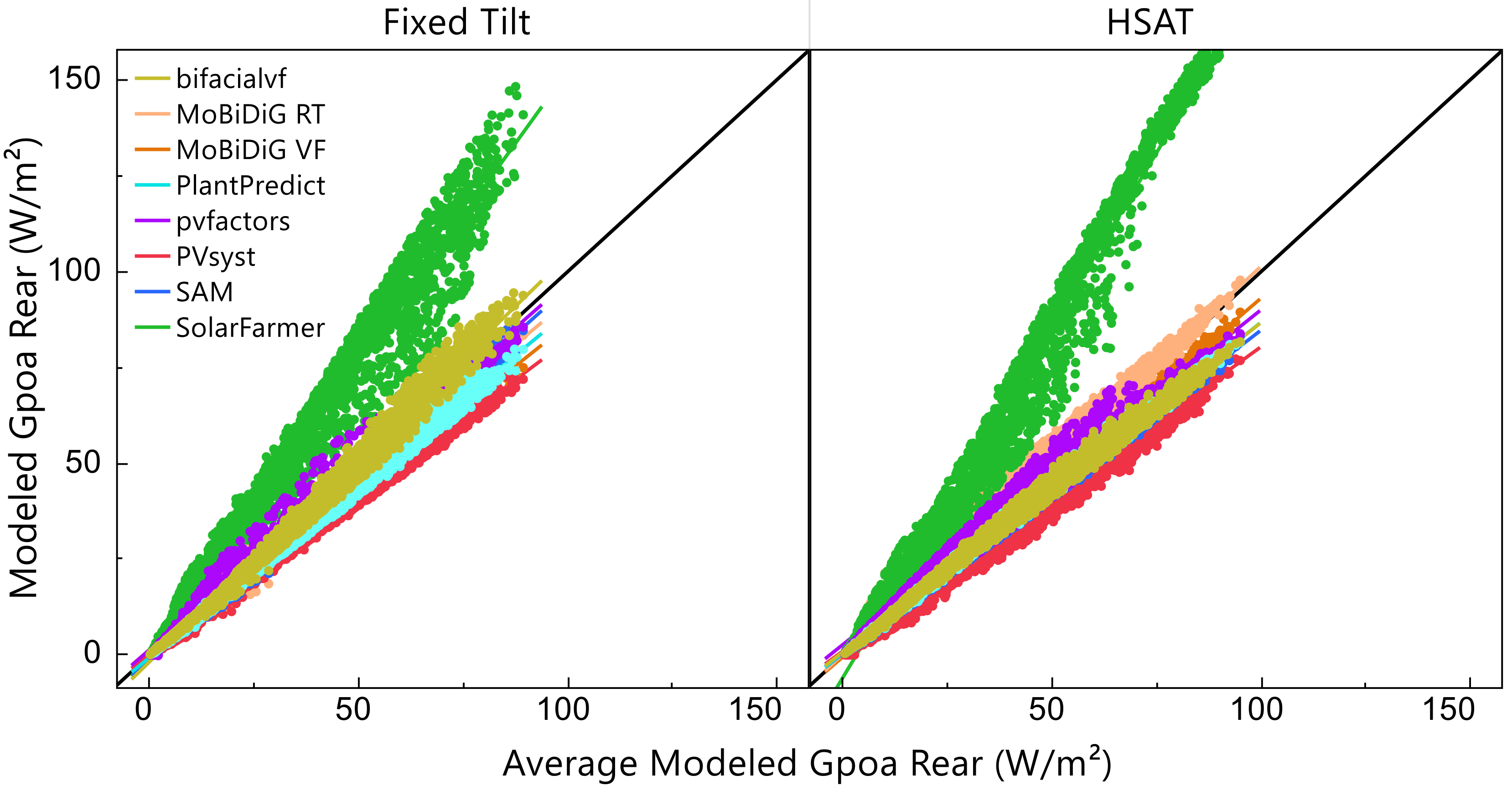
The fundamental challenge in bifacial—as compared to monofacial—PV performance modeling is estimating G_POA,Rear. Therefore, the discrepancies in simulated bifacial energy production are likely to occur in the derivation of G_POA,Rear values. Figure 5 shows one year of simulated G_POA,Rear values as a function of the average simulated value. The dispersion of simulated values is nearly the same for the fixed-tilt and HSAT system. The range of simulated values among software correlates with the front-side irradiance (R² = 0.81–0.85). The range of simulated G_POA,Rear values is approximately 20 W∙m⁻² at 1000 W∙m⁻² frontside irradiance. In other words, the range of G_POA,Rear is about 2% of G_POA,Front. SolarFarmer is highest in this comparison because its integrated approach does not currently consider the obstruction of sky diffuse irradiance caused by neighboring PV rows. Therefore, the ground-reflected irradiance between PV rows is over estimated. To our knowledge, this detail is currently being revised and is expected to be implemented in SolarFarmer versions greater than 1.0.191.2.

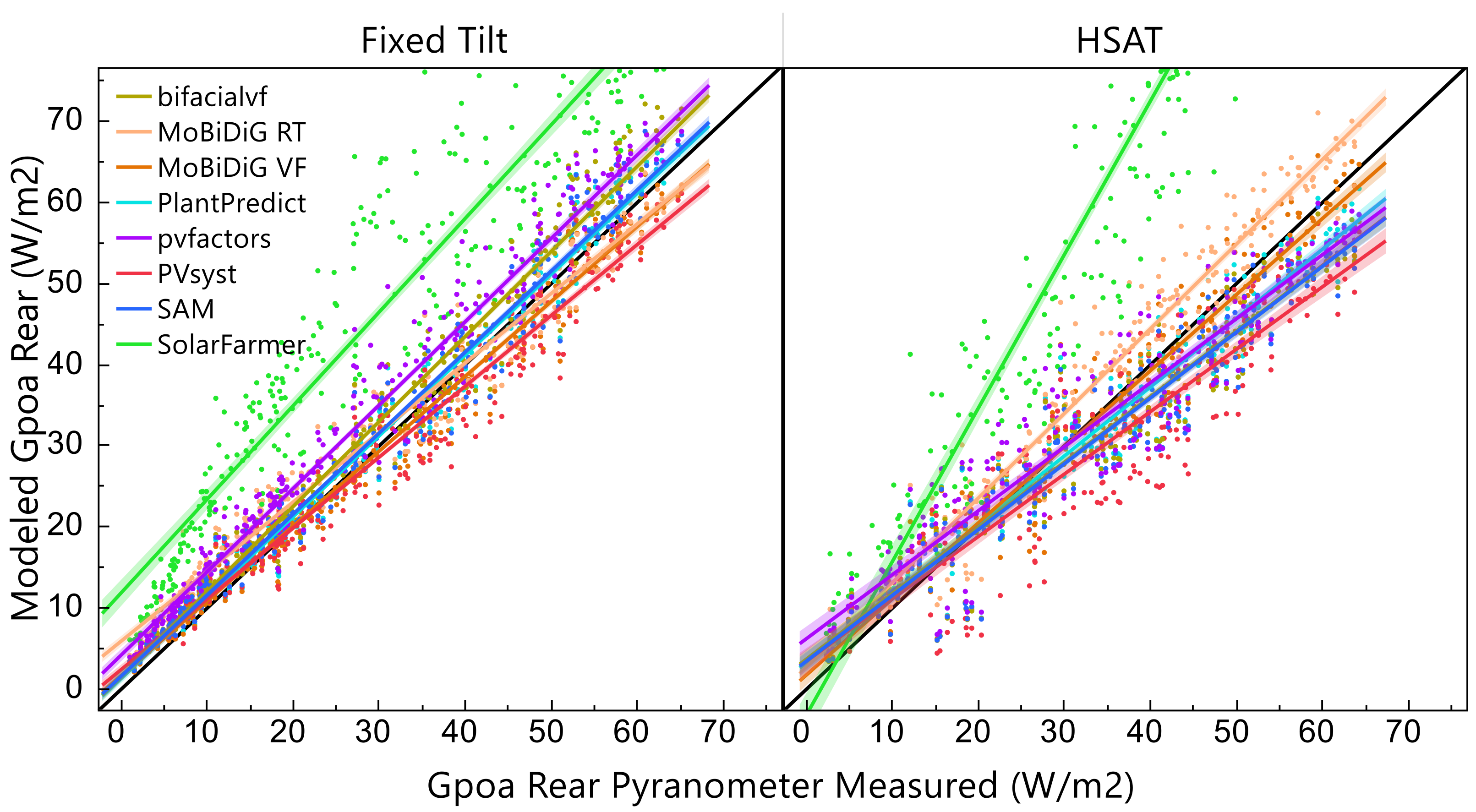
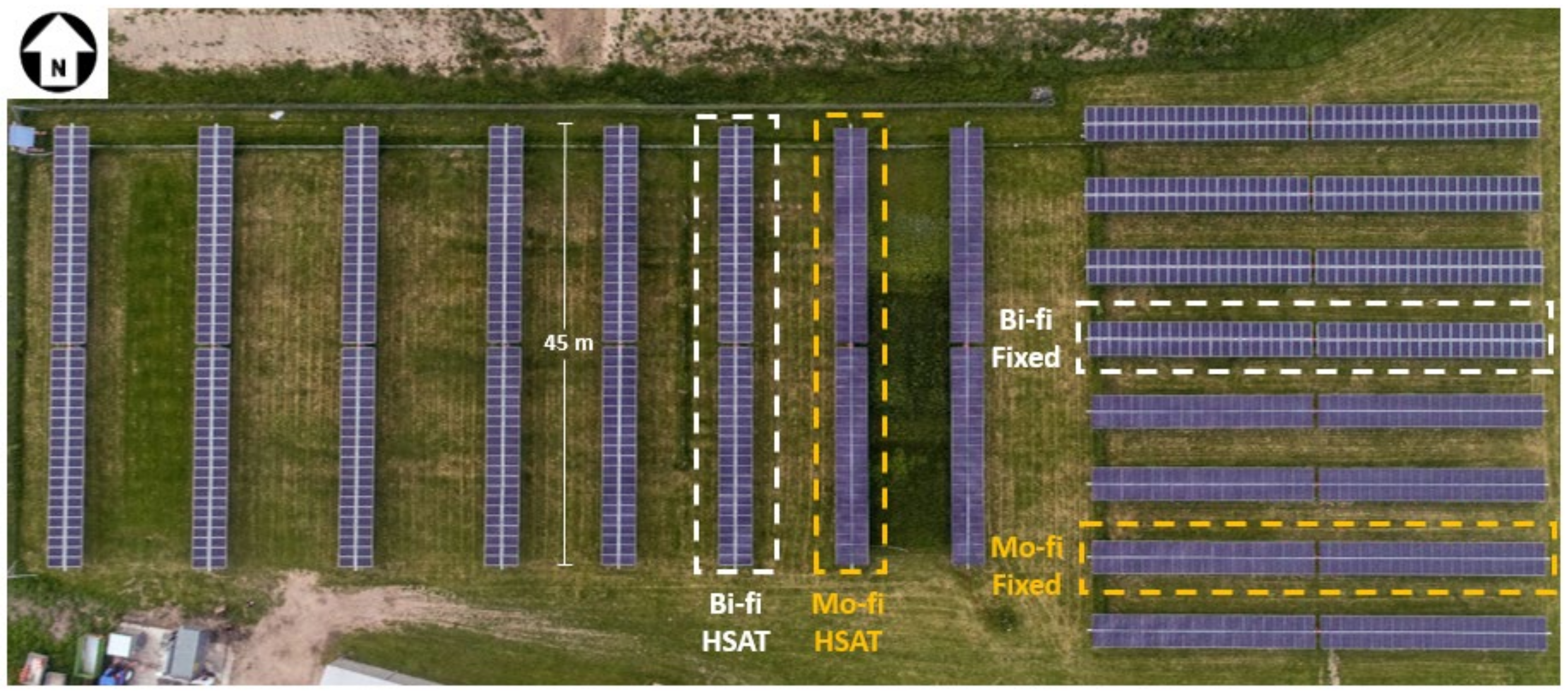
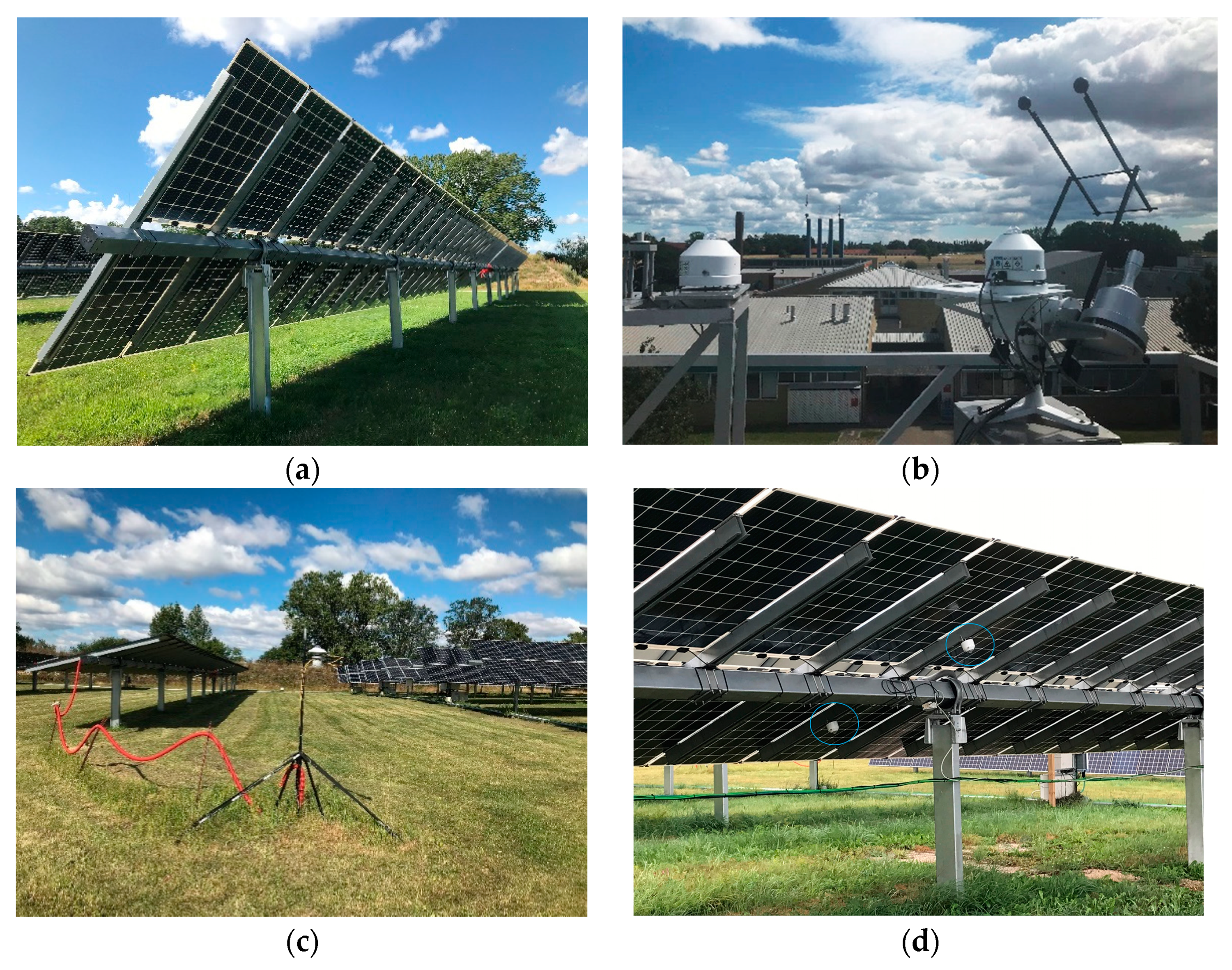
A comparison of the modeled G_POA,Rear during five weeks (21 February–30 March 2020) where measured G_POA,Rear data are available on the fixed-tilt and HSAT system is shown in Figure 6. The simulated results include reflection losses at the PV glass–air interface according to the IAM model implemented in each software. The solid black 45° lines in Figure 5 represent unity to the measurements. The measurements are the average of two MS-40 pyranometers (EKO Instruments, Tokyo, Japan) mounted on the backside of the structure: east and west in the case of the HSAT, top and bottom for the fixed tilt (Figure 2d).

The trendlines from seven of the eight software agree well with the pyranometer measurements. The mean absolute error (MAE) of these seven software is 2.3–5.2 W∙m⁻² for the fixed-tilt system and slightly higher at 3.5–6.7 W∙m⁻² for the HSAT system. We analyzed the model residuals as a function of the sun position G_poa,front and diffuse fraction and found no systematic trends, other than a tendency towards higher percentage errors in G_POA,Rear when G_POA,Front is low.

The peak total irradiance (i.e., sum of G_POA,Front and G_POA,Rear) of both system types was approximately 1000 W∙m⁻² during the five-week period shown in Figure 6. When the magnitude of total irradiance is considered, the MAE of G_POA,Rear contributes roughly 0.5% uncertainty to the bifacial PV modeling chain. The 3-D MoBiDiG RT simulation over predicts G_POA,Rear in the HSAT scenario, which could be due to its use of the Perez all-weather luminance model [59], which is unique among all software tested. The overall poorer model agreement with measurements in the HSAT scenario makes sense considering that tracking introduces additional complexity—and thus additional degrees of freedom for error—at two levels. First, the tracker algorithm implemented by the software is introduced into the comparison and second, the VFs in HSAT simulations are calculated for each change in tilt angle whereas the VFs in fixed-tilt simulations are calculated once for the entire simulation.

An inclinometer sensor mounted on the back of the tracker continuously recorded the tracker roll angle during the test period. We found that the modeled tracker angle was within ±1° of the measured angles 50% of the time, but deviations were as high as 5° during periods of backtracking. We used pvfactors to test the effect that this difference in the roll angle had on simulated G_POA,Rear values. When the measured—as opposed to calculated—angular position was used in the simulation, we found that the mean bias error (MBE) improved slightly from −1.1 to −0.7 W∙m⁻², but the MAE, however, changed by less than 0.1 W∙m⁻².

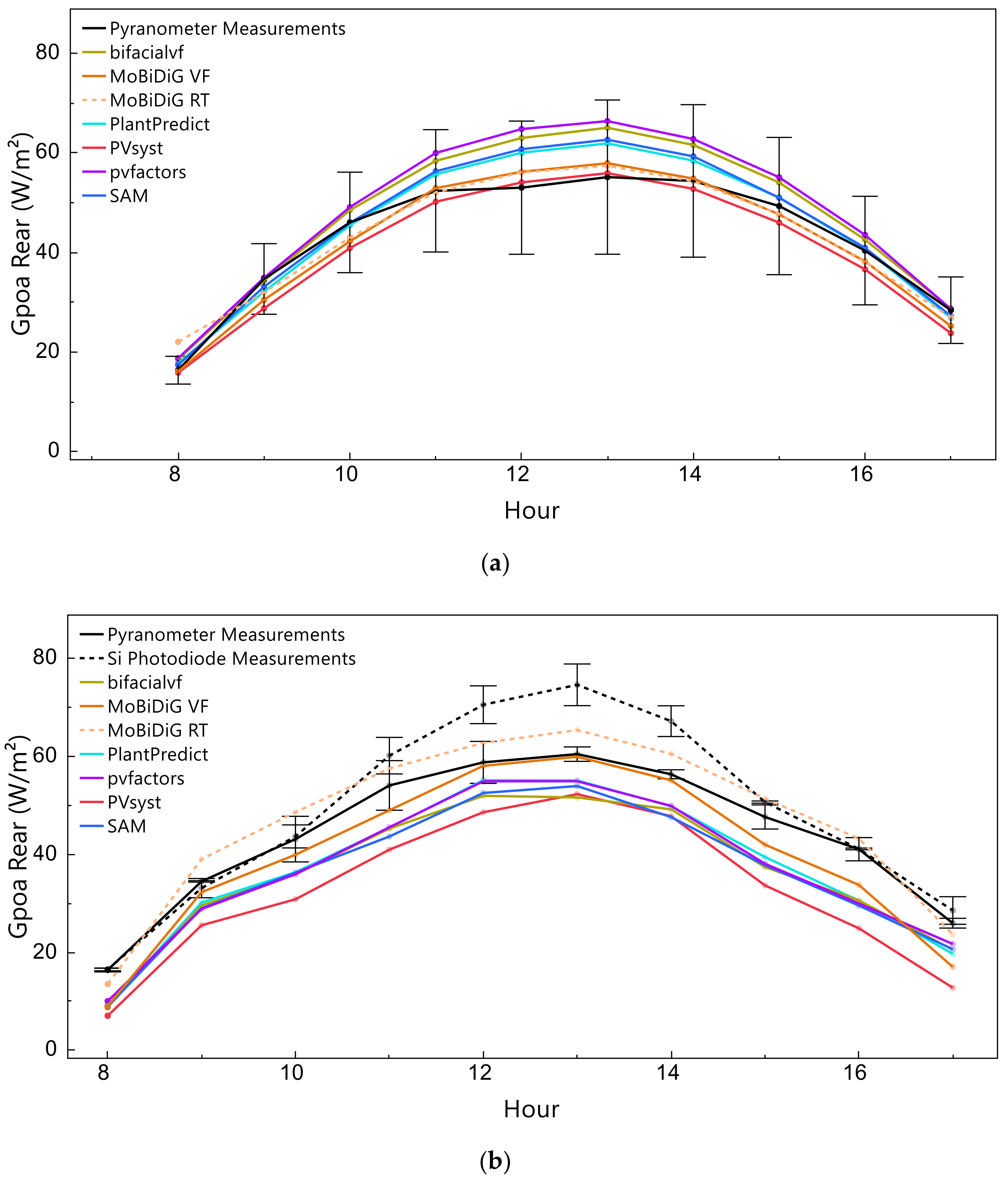
The spatial non-uniformity of irradiance on the backside of a bifacial PV array makes it difficult to identify a position for a backward-facing irradiance sensor that is representative of the entire array. Fortunately, research is being conducted on this topic by other authors, although it is still in an early stage [60]. During clear sky (i.e., low diffuse fraction) days, we observed that the bottom pyranometer can receive nearly twice as much irradiance as the top pyranometer. Therefore, the black unity line in Figure 6, which represents the average measurement from two sensors, can at times have error bars on the order of ±15 W∙m⁻². On such clear sky days, seven of the eight software studied give G_POA,Rear results that are within this range (Figure 7a). In other words, when the vertical spatial non-uniformity of irradiance is considered, the reduced-order complexity 2-D VF models perform reasonably well for fixed-tilt simulations.

In the HSAT scenario, we do not see the same level of model agreement (Figure 7b). We observed that the irradiance sensor closest to the sky (i.e., western sensor in the morning, eastern sensor in the afternoon) typically receives more irradiance than the pyranometer closest to the ground, which is consistent with the findings of [22]. We found that the differences between eastern and western G_POA,Rear measurements on the HSAT system were not as extreme as differences between the top and bottom G_POA,Rear measurements on the fixed-tilt system. On a clear sky day, we observed differences on the order of 10 W∙m⁻² between western and eastern pyranometers. Although five of eight software agree within 5 W∙m⁻² of each other, none of the same five tools overlap with the measurement uncertainty bars in Figure 7b. This result could likely change if alternative backside pyranometer locations were chosen. Therefore, the PV industry could benefit from a standardized best-practice protocol for mounting the rear plane of array irradiance sensors in bifacial PV monitoring systems.

The difference between Si photodiode G_POA,Rear measurements and pyranometer G_POA,Rear measurements is most apparent at midday, when the tracker is at or near a horizontal tilt. This could be because the Si photodiodes used in this work are calibrated under the air-mass 1.5 global reference spectrum (AM1.5G), but the spectral reflectance of grass deviates strongly from the spectral distribution of AM1.5G [61]. Particularly, healthy grass has high reflectance in the near-infrared spectrum and very little reflectance in the visible spectrum where the AM1.5G spectrum peaks. It is well known that the output of silicon PV devices calibrated under the AM1.5G spectrum will increase as the observed spectrum “red shifts” [62,63]. This can explain why the Si photodiode measurements are higher than the pyranometer measurements around midday when the tracker is near horizontal, and the sensor’s field of view is primarily encompassed by grass, not the sky. However, the spectral response of the Si photodiodes is reasonably well matched to that of the bifacial PERC module’s rear side, and for this reason, the readings from this sensor type could be more representative of the effective irradiance received at the backside of the PV array. Indeed, further research is needed on the benefits of silicon radiometers (reference cells) versus pyranometers in bifacial PV monitoring applications.

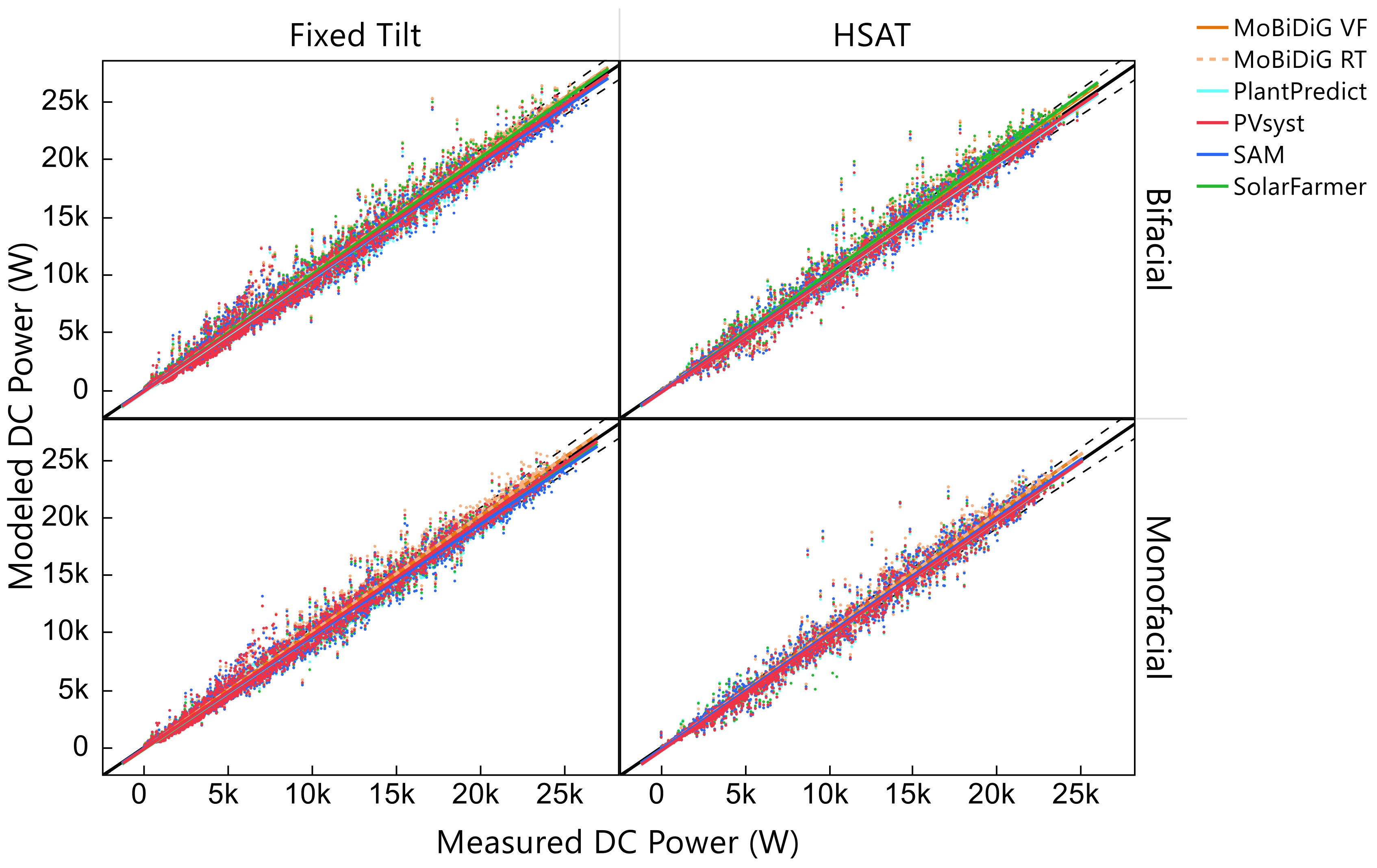
3.2. DC Power

Figure 8 shows one year of modeled versus measured DC string power of four PV configurations as simulated by six software. Good correlation is observed in all 24 regressions (R² = 0.99), but residual errors can exceed 5 kW (20%) in some cases. When such large errors are observed, the error is similar for all six software, which indicates an unidentified issue with the meteorological measurements and/or the electrical monitoring system. The DC electrical monitoring system measures string-level voltage and current independently of the inverter. The galvanically isolated data acquisition boards are a commercially available string.bloxx solution from Gantner Instruments (Rodgau, Germany). From the specifications, we determined the uncertainty of the DC power measurements as ±0.5% at the full scale. The dashed black lines in Figure 8 are drawn at ±4.5% from the solid black unity line and depict the GHI measurement uncertainty on a clear day at solar noon (±4%) and the uncertainty of the power measurements (±0.5%). All 24 trend lines in Figure 8 are within this boundary at measured power levels greater than 7 kW.

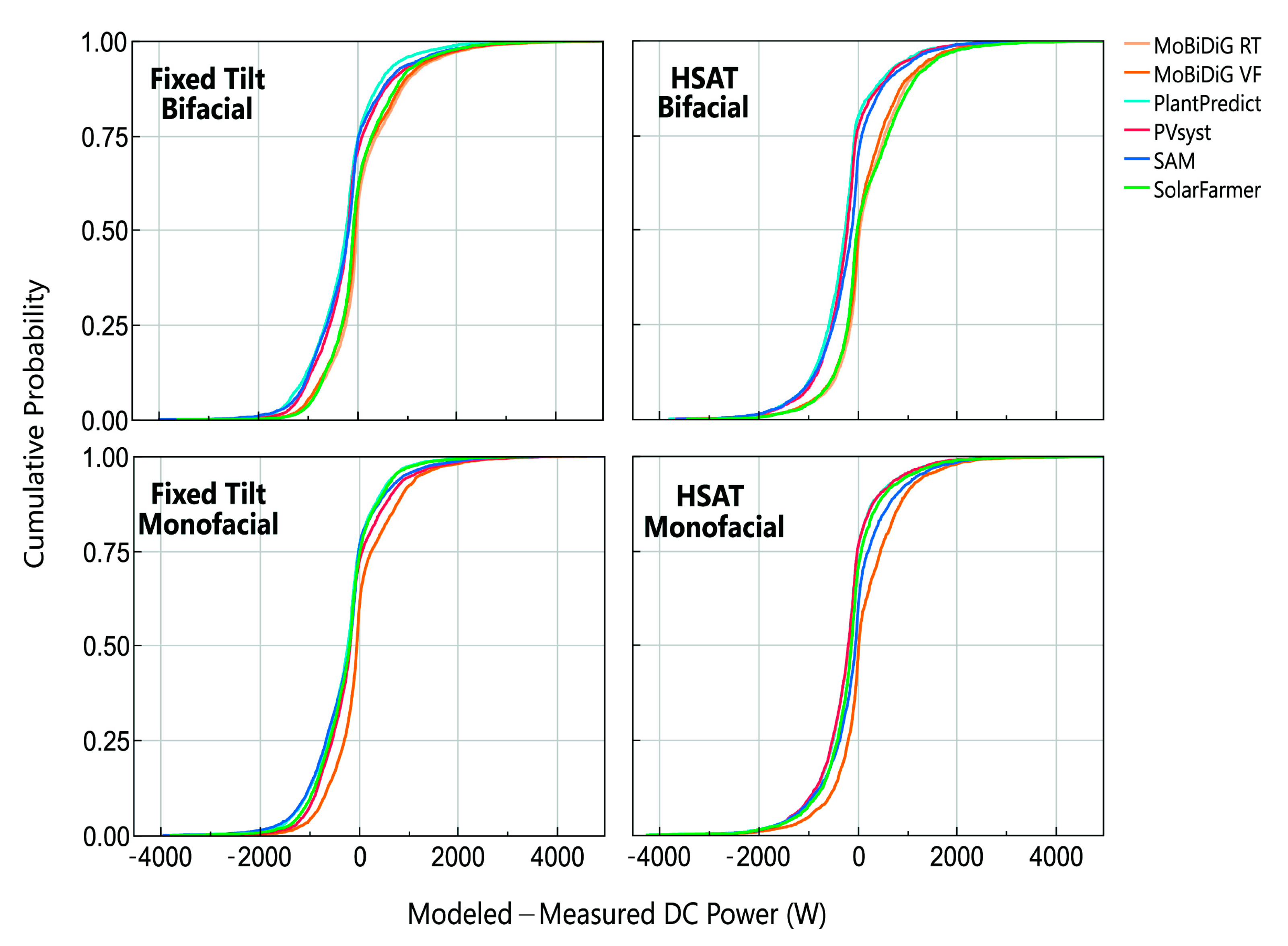
Figure 9 shows the model errors from Figure 8 in the form of cumulative distribution functions (CDFs). The slopes of all 24 CDFs in Figure 9 are steepest around approximately ±500 W, which indicates that the majority of errors are within this range. CDF shifts in the positive X-axis direction indicate that a modeling tool has a tendency toward higher DC power predictions, while shifts in the negative x-axis direction indicate a tendency toward more conservative DC power predictions. With this in mind, the bifacial fixed-tilt and HSAT simulations reveal two groups: PlantPredict, PVsyst, and SAM showing nearly identical CDFs; and MoBiDiG RT, MoBiDiG VF, and SolarFarmer showing very similar CDFs. The former group has a tendency toward negative bias and the latter group a tendency toward positive bias. In the case of the bifacial HSAT simulation, the reason for this two-group split could be attributed to the latter group yielding the highest estimates of G_POA,Rear (Figure 6). In the case of the bifacial fixed-tilt simulation—and both monofacial simulations—the explanation is not so clear and therefore likely not attributable to a single difference in submodeling steps but rather due to the differences accumulated in multiple submodels. We performed regressions of the DC power residuals as a function of measured variables, such as diffuse light fraction (DHI/GHI), sun position (zenith and azimuth), and G_POA,Front. This exercise revealed no significant correlations (R² < 0.25) or systematic trends, other than a trend of larger absolute errors during times of high solar irradiance.

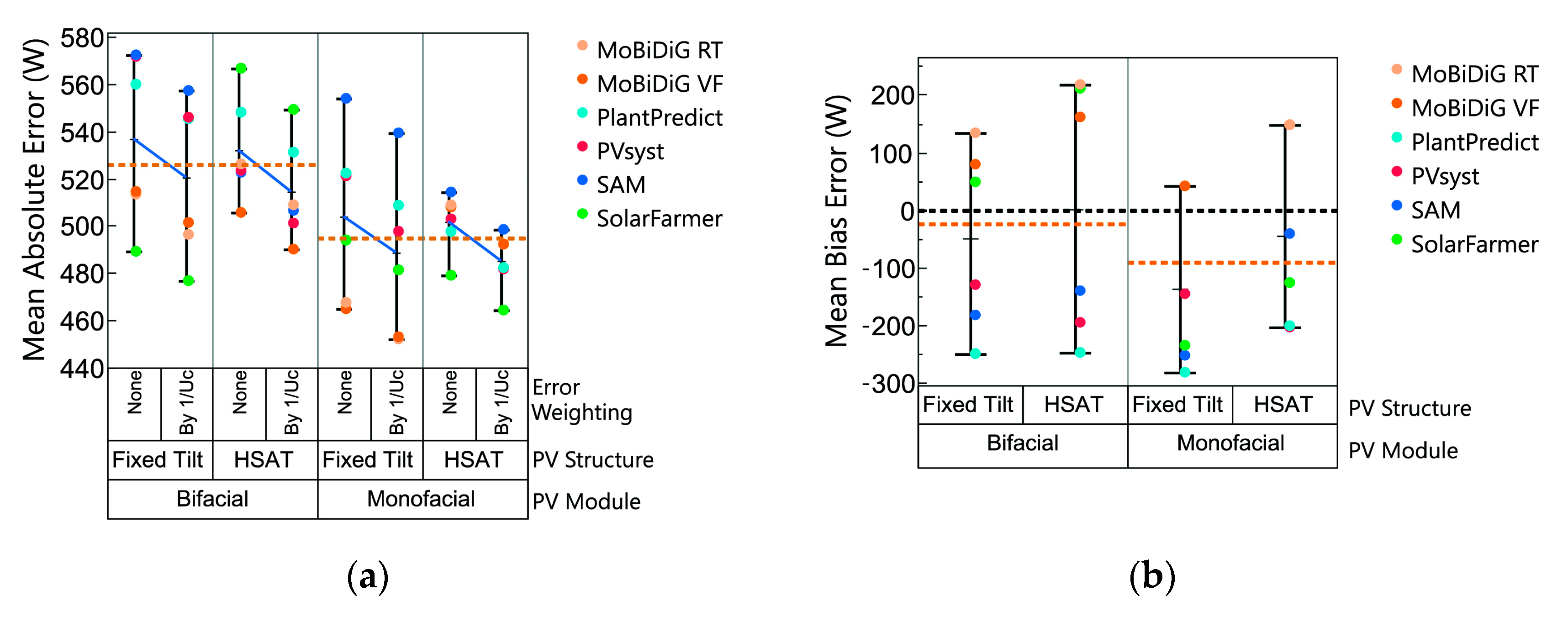
Figure 10 shows two variability plots that summarize the annual mean absolute errors (MAEs) and mean bias errors (MBEs) of the four PV system types simulated by six software. The dashed orange lines in each variability plot represent the average modeling error of the bifacial and monofacial system types and indicate a 30 W higher MAE in bifacial simulations. The slightly higher MAE can be explained simply by the fact that the bifacial arrays produce about 5% more energy on an annual basis than the monofacial arrays. When the MAE is normalized to the average power produced by each system type over the year, we found that the normalized error is about 0.25% higher for bifacial simulations versus monofacial simulations. This difference is likely driven by the contribution of G_POA,Rear. In terms of the average MBE, bifacial simulations are about 90 W higher than monofacial simulations but closer to zero bias than the monofacial simulations. Within the context of the results obtained from the site studied here, we conclude that the accuracy of bifacial PV simulations is not significantly different than monofacial PV simulations.

Figure 10a shows the MAE calculated using two approaches: (1) without error weighting and (2) by weighting the error with the inverse uncertainty (1/U_C) of the solar radiation measurements during each hour of energy production. In approach (2), the errors are weighted by either the GHI uncertainty or DNI uncertainty, depending on the data used in the transposition step, and the sum of all error weights equals one. The rationale behind the 1/U_C weighting in approach (2) is that uncertainty in solar radiation measurements directly impacts simulated PV power, which ought to be accounted for in error analyses. As expected, weighting the error by a factor of 1/U_C reduces the MAE, but the reduction is small at about 20 W, or 0.2%.

3.3. Bifacial Gain

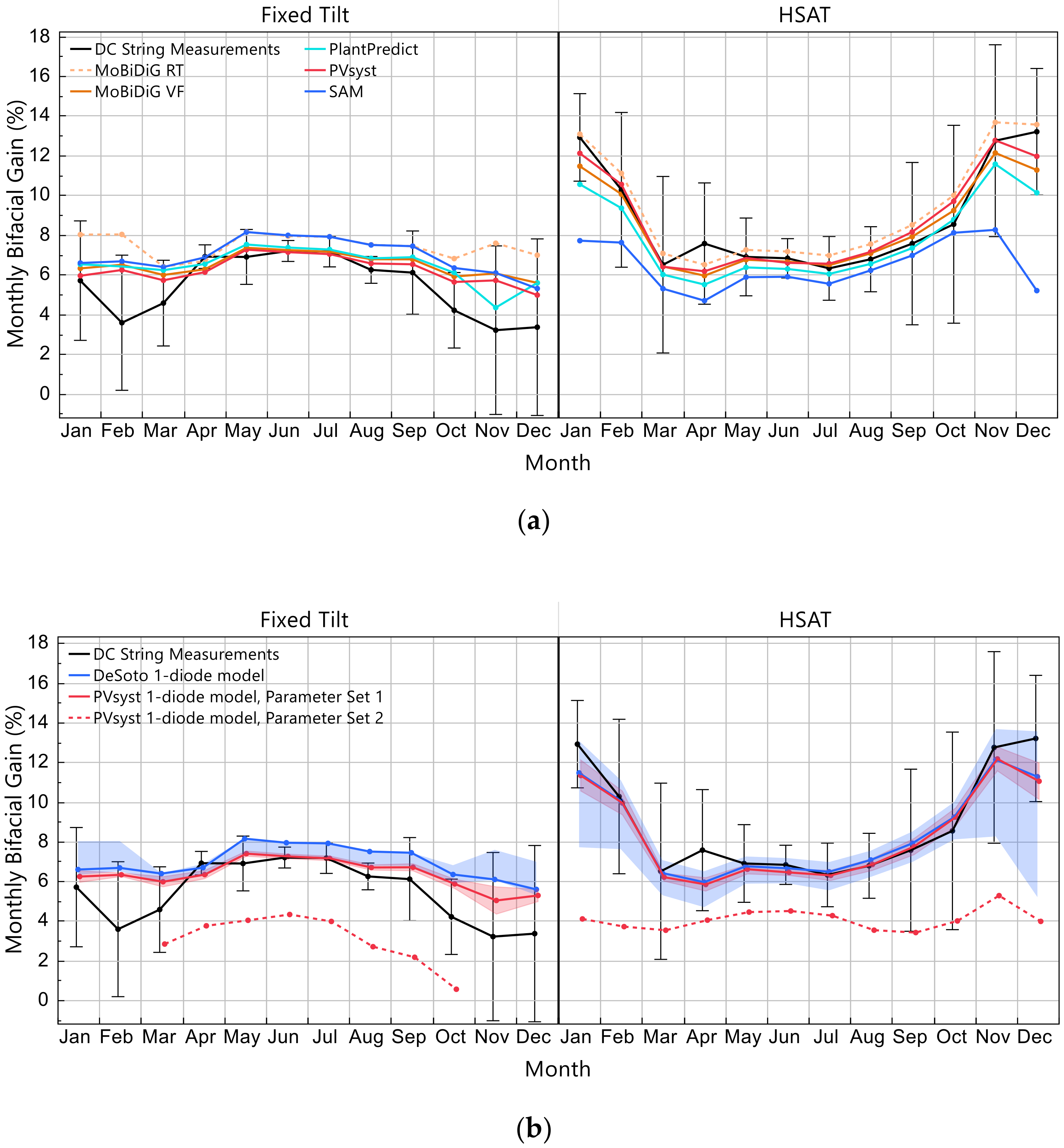
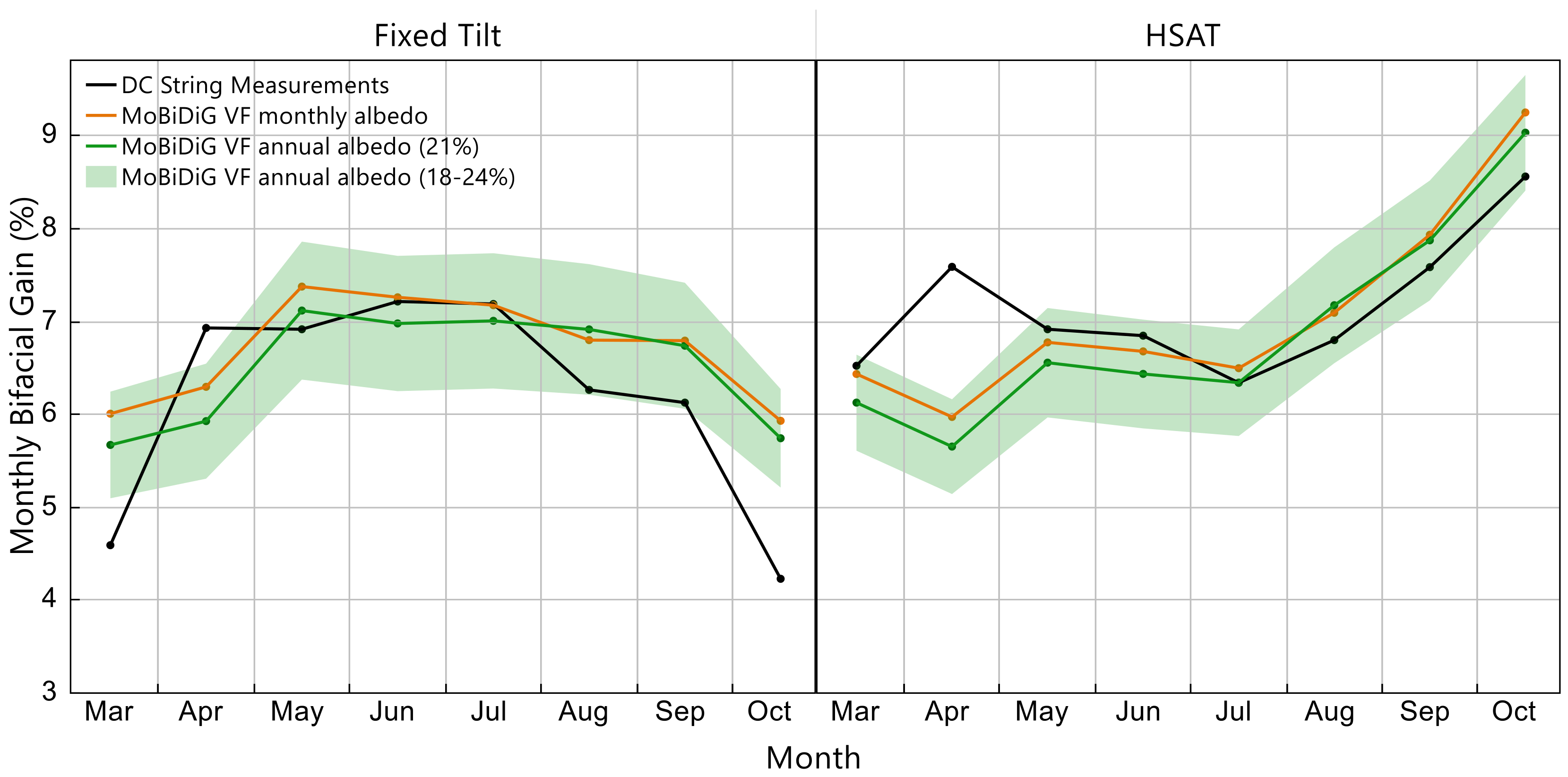
Figure 11 shows the monthly bifacial gain from five software that are capable of simulating electrical performance. The black lines in each plot show the monthly results from the DC string measurements. The error bars show the inner quartile range of daily measured bifacial gains observed in each month. The daily bifacial gains in winter fluctuate greatly because the daily energy production in winter can be an order of magnitude less than in summer months: This variability is illustrated with the wider error bars in winter. Recall that the measured results are normalized with the I-V measurements made at DTU per Equation (1). If the normalization was instead made using the manufacturer’s nameplate rating, the measured bifacial gain according to Equation (1) would be 1.5% higher than what is shown. This difference can significantly affect the economics of project decisions that are made based on an expected bifacial energy gain.

The measured monthly bifacial gain on the fixed-tilt system is between 4.3% and 7.3% from March to October. Meanwhile, the bifacial gain on the tracker is consistently higher, between 6.6% and 8.5% during the same months. The higher bifacial gains observed on the HSAT are likely due to the wider 12-m spacing between rows (GCR = 0.28) versus the narrower 7.6-m spacing on the fixed-tilt system (GCR = 0.4), which creates more self-shading within the inner rows of the fixed-tilt field.

From November to February, the measured bifacial gain on the two system types shows opposing trends, wherein the HSAT system shows an increase and the fixed-tilt system shows a decrease. These months were characterized consistently as cloudy skies with mean monthly diffuse fractions between 88% and 94%. The works of other authors have demonstrated that bifacial gain will increase as the fraction of diffuse light increases [64], which can explain the higher bifacial gain on the HSAT system in winter. It also been shown that bifacial PV systems require higher tilt angles to capture the benefit of such diffuse conditions [65]. This can explain why the simulations and the measurements in winter show lower bifacial gains on the fixed-tilt system (25°) than the HSAT system (±60°).

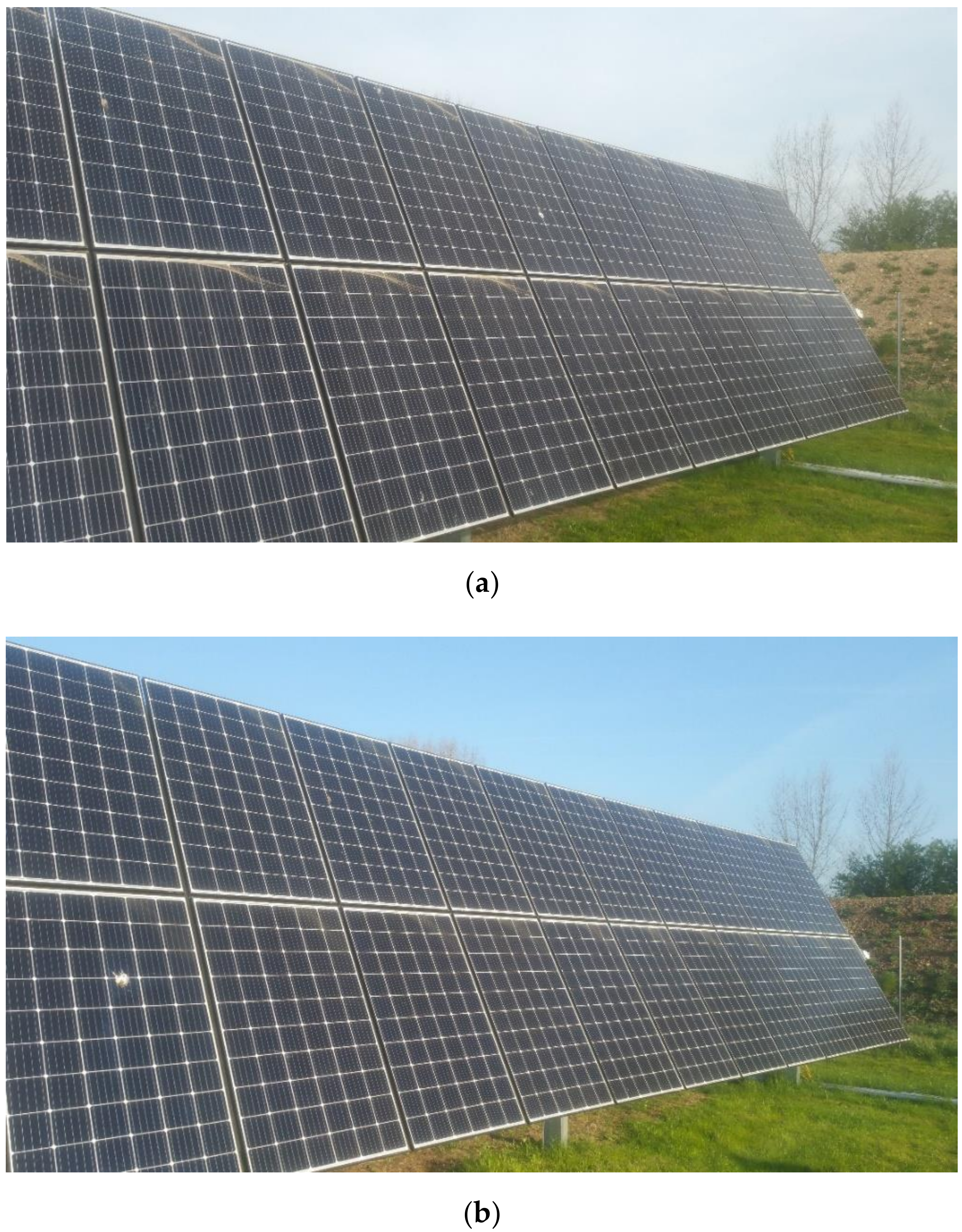
The simulated bifacial gain values largely follow the trends of the measurements, but the most notable exception is the fixed-tilt system in winter (November through February). This discrepancy is likely due to the significant amount of inter-row shading on the fixed-tilt system from November to February. The fixed-tilt system has a shade angle (at solar noon) of 16°, but on the winter solstice, the sun elevation peaks at 12°. Therefore, the fixed-tilt rows are partially shaded at practically all times in December and January. In fact, negative bifacial gains were measured in November and December on the fixed-tilt systems. Such an incongruous result points toward issues in the measurements rather than the shade-loss models. A visual inspection on a clear winter day near solar noon confirmed that there was more inter-row shading on the bifacial arrays than on the monofacial arrays. This is attributed primarily to the torque tube gap on the bifacial arrays, and the lack of such a gap on the monofacial arrays. The torque tube gap on the bifacial arrays (Figure 2a) places the bifacial modules approximately 5 cm higher than modules on the monofacial arrays that completely cover the torque tube (Figure A2). This slight differentiation in structural geometry may not have been simulated sufficiently in the software.

Another notable discrepancy between the model and measurement is seen in April when a small spike in bifacial gain is observed on both the fixed-tilt and HSAT system. The trend in modeled bifacial gains from March to May indicate that the measured bifacial gain in April is overstated by as much as 1.5%. We believe the higher measured bifacial gain in April was caused largely by extraordinarily high pollen counts in late April 2019, which caused non-uniform soiling on the PV arrays, and ultimately more power loss in the monofacial than bifacial systems. We observed that the daily bifacial gains were between 10% and 20% from 23–26 April 2019, which corresponds to the dates of the soiling event (Figure A2). A significant rainfall event occurred on 27 April 2019 at which point more modest and typical bifacial gains resumed. This artifact highlights the challenge of curating high-quality data acquisition in large-scale PV test sites.

Please note that the bifacial gain results from SolarFarmer are not presented in Figure 11 because the overestimation of G_POA,Rear shown in Figure A2 causes a 2–4% upward bias in bifacial gain as compared to the other tools, which use the PVsyst 1-diode model (i.e., PlantPredict and PVsyst). This result conflicts with our previous work [27], which showed SolarFarmer results mostly within 1% of the measured bifacial gain, while PlantPredict and PVsyst results were 3–4% low to the measured bifacial gain. The reason for this discrepancy is that the present work uses a 1-diode model parameter set based on laboratory measurements made at irradiances from 200–1000 W∙m⁻² (noted as ‘Parameter Set 1’ in Figure 11b) while our previous work used a parameter set based on measurements made only at STC (noted as ‘Parameter Set 2’ in Figure 11b). The improved agreement of ‘Parameter Set 1’ shown here is attributed to the fact that this parameter set more accurately predicts performance at low-light conditions (<400 W∙m⁻²) than does ‘Parameter Set 2’. This finding is in agreement with the findings and recommendations of other authors [66,67].

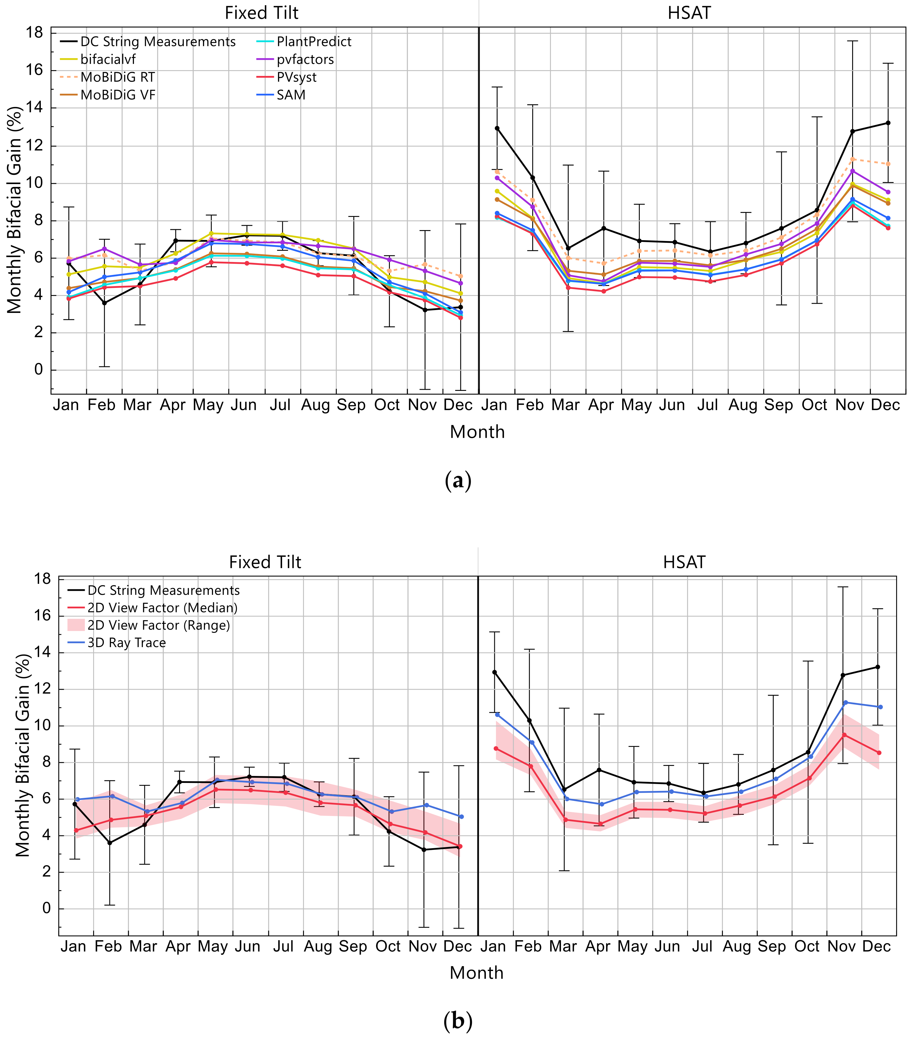
Figure 12 shows the simulated bifacial gain according to the G_POA,Rear to G_POA,Front ratio (Equation (2)). The agreement among the different software is similar regardless of whether the bifacial gain is calculated using the optical gain (Equation (2)) or the electrical performance (Equation (1)), with the exception of HSAT results in winter, where better agreement among software is seen using Equation (2). The larger discrepancies between HSAT simulations in winter using Equation (1) could be due to the different backtracking and shade-loss algorithms used by the software. Equation (2) results in better agreement with the fixed-tilt system measurements in winter, which indicates that inaccuracies in the shade-loss models are likely the result of the significant winter deviations shown in Figure 11.

Figure 12b shows the results grouped by whether G_POA,Rear is calculated using a 2-D VF or 3-D RT approach. When visualized in this manner, it becomes clear that the 3-D RT approach follows the measured bifacial gain most closely for the HSAT simulation, within 0.5% of measurement for most months outside of winter. The 3-D RT model also matches well, typically within 0.5%, with the bifacial gain measurements on the fixed-tilt system. However, 2-D VF models, such as the one integrated in SAM, compared equally well to field measurements. Indeed, the measured bifacial gain shown in Figure 12 is influenced by the value of Bifi_loss. The static Bifi_loss values used here, in actuality, change dynamically over the day with the prevailing conditions [19,57,58]. All the commercial software tested here has the capability to use only a single value. This simplification offers room to improve the accuracy of the bifacial PV performance simulation tools used in industry today.

3.4. Frontside Plane-of-Array Irradiance (G_POA,Front) and Module Temperature (T_MOD)

PV project developers and investors are often interested in bottom-line figures, such as performance ratios, specific yields, and, in the case of bifacial PV, the bifacial gain. However, comparing simulations to measurements at such a high level is often not meaningful without first analyzing the performance of key submodeling steps. This section builds on this analysis, which started in Section 3.1 with an assessment of G_POA,Rear, and shows how the simulations compare to onsite front-side plane-of-array irradiance (G_POA,Front) and back of module temperature (T_MOD) measurements.

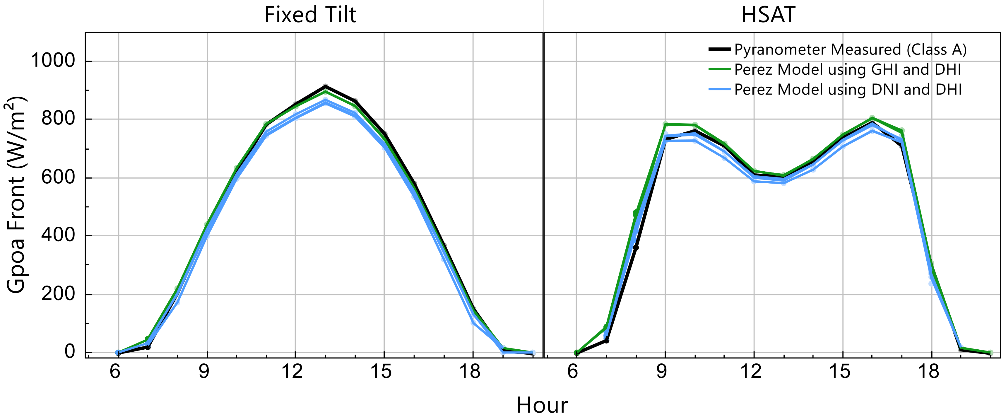
Figure 13 shows an overlay of the simulated and measured G_POA,Front on a cloudless day. The trends shown here are representative of the results from clear sky days within the test period. The plot is color coated by which combination of solar radiation measurements is used in the Perez transposition model. Lower G_POA,Front estimates (≈40 W∙m⁻²) are seen at midday when DNI is used in the transposition step. On an annual basis, the MBE is between 11 and 13 W∙m⁻² when GHI is used in transposition, and when DNI is used in the transposition step, the MBE is between −7 and 5 W∙m⁻². These rather large differences in results using DNI and DHI versus GHI and DHI could be the result of measurement issues with either the GHI pyranometer or DNI pyrheliometer. However, it is worth reiterating that weekly maintenance is performed at the weather station, and that the GHI, DHI and DNI data passed the quality checks recommended by the BSRN [46]. Additionally noteworthy in Figure 13 is how there are considerable deviations among the tools that use the same DNI and DHI data as input, a result that is similar to that of other authors [28].

Since the front-side irradiance constitutes 92% or more of the total irradiance for half of the timestamps in the bifacial simulations, one would suppose that software that uses DNI in the transposition step would tend to underpredict DC power. However, this turns out to not always be the case. For example, MoBiDiG is one such tool that uses DNI, and this tool was shown in the CDF plots of Figure 9 to overpredict DC power of all PV system types compared to the other five software. SAM is another such tool that uses DNI, but the results in Figure 8 and Figure 9 show that SAM tends to predict marginally higher DC power values than the tools that use GHI but only in HSAT simulations. The underprediction of G_POA,Front by MoBiDiG and SAM could be compensated by their tendency to overpredict electrical performance at irradiance conditions <400 W∙m⁻², which is due to their use of the De Soto versus PVsyst 1-diode model (Figure A1). This demonstrates how analyzing the accumulated errors at various submodeling stages and their subsequent impact on energy yield is not always a straightforward process.

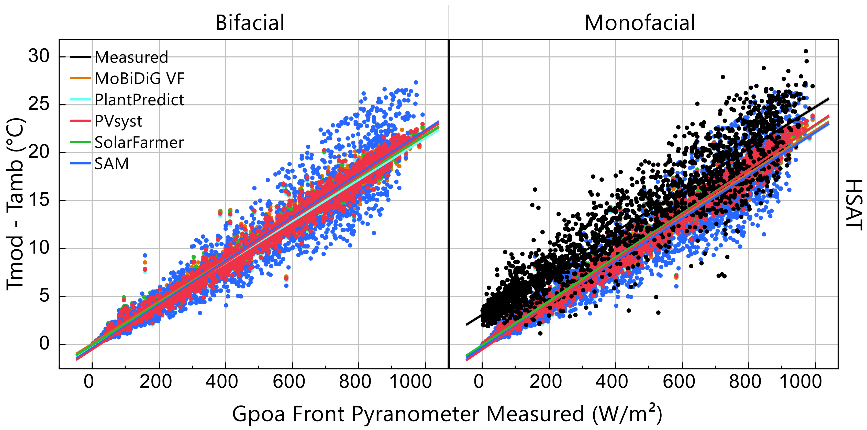
Figure 14 shows the difference between module temperature and ambient temperature versus G_POA,Front. This difference between module and ambient temperature is known to be essentially linear with respect to the in-plane irradiance with a slope proportional to the U₀ coefficient used. The variations around the regression lines are due to the assumptions for convective heat transfer in the U₁ coefficient. A notable difference in Figure 14 is the module temperature predicted by SAM, which is simply due to SAM’s use of the NOCT versus Faiman model. The T_MOD measurement comes from one 4-wire resistance temperature device (RTD) affixed to a single cell on the backsheet of a module within the array; no translation from back of module (backsheet) to cell temperature is made in Figure 14. The monofacial results of Figure 14 show that the simulations tend to underpredict the measured back of module temperature by 2–3 °C, but errors are often greater than 5 °C. Unfortunately, T_MOD sensors were never installed on the bifacial arrays, and as such, only monofacial temperature measurements are available.

All software studied here implement simplified steady-state thermal models that assume the PV array operates at a homogenous temperature, which can lead to discrepancies with measured values. Although healthy (i.e., non-damaged) modules are typically assumed to have homogenous temperatures within an array [68], cell temperatures are known to vary within a healthy module [69]. Therefore, the cell on which the RTD is placed may not be representative of the average cell temperature within the array, which is a potential source of error when comparing to modeled values.

Appropriate values for device-specific thermal parameters, and the methods to acquire them from measurements, have been the subject of discussion and debate in the PV community [70]. Therefore, we performed a sensitivity analysis of the U₀ and U₁ thermal coefficients using the MoBiDiG VF tool. Our sensitivity found that the MBE of simulated monofacial DC power was minimized using U₀ and U₁ parameter values of 24 W∙m⁻²∙K⁻¹ and 1.6 W∙m⁻³∙K⁻¹∙s, respectively. The sensitivity analysis showed that the best agreement between the modeled and measured module temperature would require U₀ and U₁ values near 20 W∙m⁻²∙K⁻¹ and 0 W∙m⁻³∙K⁻¹∙s, respectively. Since these values are below the lower boundary of published values that we are aware of for open-air mounted PV systems [54,71], it seems that the cell on which the RTD is placed is not representative of the average cell temperature within the array.

3.5. Sensitivity Analysis of the Albedo

While the bifacial gain is known to increase linearly with increases in albedo [65,72,73], uncertainties in albedo measurements have been shown to have a non-negligible effect on bifacial performance [74]. Therefore, we performed a sensitivity analysis with the MoBiDiG VF tool using annual albedo values from 18% to 24% (±3% of measured annual average) in place of the monthly measured albedo data that were used in previous sections. The results from this analysis are shown in Figure 15, with winter months excluded for clarity.

Figure 15 shows that differences in simulated bifacial gain are very small (<0.3%) when annual average albedo data are used in place of monthly averages. However, during the high solar resource months of May through August, using monthly albedo in the simulation tends to match the measured bifacial gain more closely. This demonstrates that monthly albedo data is preferred over annual albedo data, even at sites where the albedo does not vary greatly throughout the year, such as the site studied here.

Figure 15 shows only few instances where the measured bifacial gain is outside the boundaries of the sensitivity. One such example occurs in April, where unusually high bifacial gain was measured. In the case of the HSAT, nearly 30% albedo would be needed to recreate the measured bifacial gain in that month. Since such uncertainty in the measured albedo is unlikely, this lends credence to our hypothesis that abnormally high pollen counts (i.e., soiling) in April caused the spikes in bifacial gain. Another instance where the measured bifacial gain is outside the sensitivity boundaries occurs in the fixed-tilt system in March and October. Since the fixed-tilt array experiences the most shading in these months, it is likely that power losses due to shading are not accurately accounted for in the simulation.

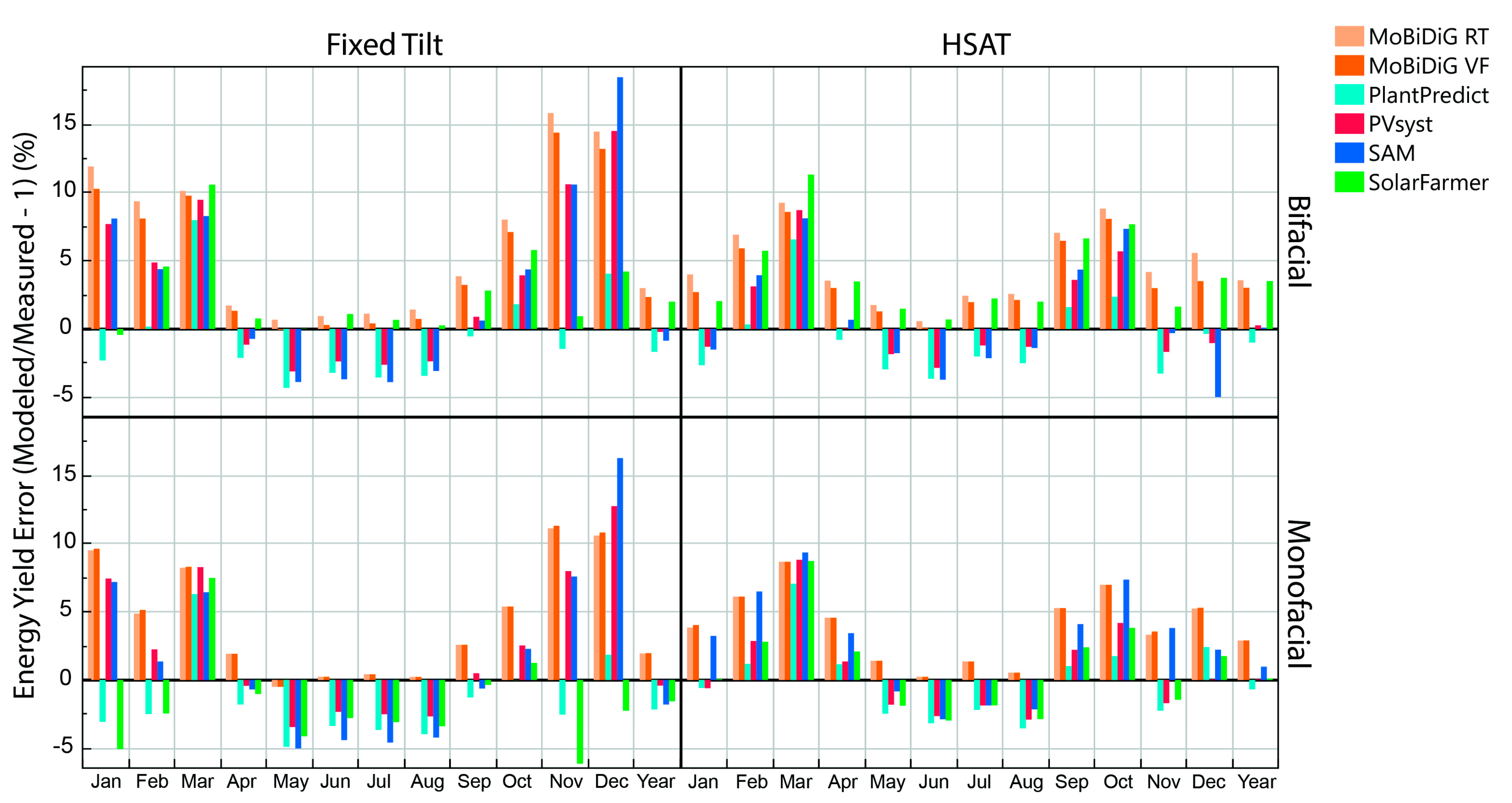
3.6. Monthly and Annual Energy Production

With the results from several key intermediary modeling steps presented, we conclude the results section with a comparison of the modeled and measured monthly DC energy. In Figure 16, the monthly and yearly errors in energy predictions across all four PV system types are shown. Please note that roughly 75% of the total annual energy is produced between April and August. With just 25% of the annual energy produced between September and March, errors during these months tend to be larger on a percentage scale. An interesting result in Figure 16 is that on a monthly basis, PlantPredict, PVsyst, SAM, and SolarFarmer fluctuate between negative and positive bias relative to the measurements, sometimes with monthly deviations greater than 5%. However, on an annual basis, all tools simulate the four PV systems within 3.5% or less of measurements, and in some cases, the annual error is less than 1%. This is a rather positive result considering the uncertainty of the solar radiation measurements and the electrical monitoring system.

The accuracy of annual results from PVsyst and SAM shown in Figure 16 are in fact better than those published by [75], which could be because the parameters and loss factors used here were thoroughly calculated rather than using default values. On an annual basis, results from PlantPredict match PVsyst within 0.7% to 2.0%, which is a slightly larger deviation than that presented in [31] for Cadmium Telluride technology, but the larger differences here could be due to the use of different IAM models to describe reflection losses and/or the introduction of G_POA,Rear. The annual MoBiDiG results are between 2% and 3% above measurements, which is higher than the ±1% published in [14] for most static-tilt configurations, but agreement could improve if, for example, the DeSoto parameter set was modified such that the modeled DC efficiency was lowered at low-light conditions (Figure A1).

Finally, a word on the accuracy of bifacial versus monofacial simulations: The difference between the annual energy yield error in bifacial versus monofacial simulations is 1% or less, for five of six software. The outlier is SolarFarmer, which shows larger differences between its bifacial and monofacial simulations, but this is simply due to the overestimate of G_POA,Rear mentioned previously. The annual errors in bifacial and monofacial simulations are no more than 0.5% different when performed in MoBiDiG VF, PlantPredict, and PVsyst. This result is in accord with the results presented in Section 3.1, which showed a deviation of roughly 0.5% between modeled and measured G_POA,Rear values when considering the contribution of G_POA,Front.

4. Discussion and Conclusions

We assessed eight bifacial PV simulation software against G_POA,Rear, G_POA,Front, T_MOD, DC P_MP, bifacial gain, and energy measurements made at a 420-kW_p test site in Roskilde, Denmark. Our results show that state-of-the-art bifacial performance models add approximately 0.5% uncertainty to the PV modeling chain. This finding was demonstrated in the analysis of modeled and measured G_POA,Rear and DC P_MP values. Although 0.5% may seem small, an uncertainty of 0.5% in a 500-MW power plant translates into 2.5 MW, which translates into substantial risk in economic models. Therefore, continued efforts in reducing error in bifacial PV simulations should continue. One suggestion is the implementation of models that describe how Bifi_loss parameters change with prevailing conditions rather than the use of static Bifi_loss parameters as used in this work.

Our results further show that, outside of winter months, 2-D view factor fixed-tilt simulations are within ±1% of the measured monthly bifacial gain. Simulations of single-axis tracker systems are less accurate with 2-D view factor simulations within approximately 2% and 3-D ray tracing within approximately 1% of the measured bifacial gain, respectively.

When comparing modeled G_POA,Rear to measurements, the accuracy is highly dependent on the location and type of the optical sensor. We therefore recommend future research efforts to develop standardization and/or best practice guidelines for the placement of rear POA sensors. We observed significant differences between G_POA,Rear measurements made with thermopile pyranometers and Si-based sensors. As such, future work should aim to improve the PV community’s understanding of how the spectral distribution of albedo impacts rear-facing pyranometer reference cell versus measurements, in the framework of bifacial PV performance assessment.

An objective of this study was to assess the accuracy of reduced-order bifacial PV simulations, and we found good agreement with measurements considering the uncertainty of the solar radiation input data. Because of this finding, and the fact that the rear irradiance contribution constitutes roughly 8% of the total irradiance for the site studied here, we suggest that the PV modeling community do not forget the importance of improving the accuracy of all parts of the PV modeling chain, including, but not limited to, shade loss models, cell temperature models, and diffuse sky models.

A shortcoming of this validation study is that it was performed at one site, with its specific conditions and equipment. We therefore recommend that future work includes a comprehensive review of all bifacial PV simulation validation studies performed to date. Such a study can inform the decisions of PV project developers and investors of bifacial PV assets.

References

1. Stoker, L. EUROPE ROUND-UP: Denmark’s First Bifacial Solar Farm is Sold, RWE to Pocket French Solar. Available online: https://www.pv-tech.org/news/europe-round-up-denmarks-first-bifacial-solar-farm-is-sold-rwe-to-pocket-fr (accessed on 31 October 2020).
2. EPRI. Bifacial Solar Photovoltaic Modules. Program on Technology Innovation. Available online: https://www.epri.com/research/products/3002009163 (accessed on 10 October 2019).
3. Kopecek, R.; Libal, J. Towards large-scale deployment of bifacial photovoltaics. Nat. Energy 2018, 3, 443–446. [Google Scholar] [CrossRef]
4. Meydbray, J. Outdoor Testing for Model Validation. In Proceedings of the 2019 BifiPV Workshop, Amsterdam, The Netherlands, 16–18 September 2019. [Google Scholar]
5. Wilson, G.M.; Al-Jassim, M.; Metzger, W.K.; Glunz, S.W.; Verlinden, P.; Xiong, G.; Mansfield, L.M.; Stanbery, B.J.; Zhu, K.; Yan, Y.; et al. The 2020 photovoltaic technologies roadmap. J. Phys. D Appl. Phys. 2020, 53, 493001. [Google Scholar] [CrossRef]
6. Urrejola, E.; Valencia, F.; Vidal, E.F.; Deline, C.; Pelaez, S.A.; Meydbray, J.; Clifford, T.; Kopecek, R.; Stein, J. bifiPV2020 Bifacial Workshop: A Technology Overview; Technical Report: NREL/TP-5K00-77817; National Renewable Energy Laboratory: Golden, CO, USA, 2020. [Google Scholar]
7. Hansen, C.W.; Gooding, R.; Guay, N.; Riley, D.M.; Kallickal, J.; Ellibee, D.; Asgharzadeh, A.; Marion, B.; Toor, F.; Stein, J.S.; et al. A detailed model of rear-side irradiance for bifacial PV modules. In Proceedings of the 2017 IEEE 44th Photovoltaic Specialist Conference (PVSC), Washington, DC, USA, 25–30 June 2017; Institute of Electrical and Electronics Engineers (IEEE): Washington, DC, USA, 2017; pp. 1543–1548. [Google Scholar]
8. Marion, B.; MacAlpine, S.; Deline, C.; Asgharzadeh, A.; Toor, F.; Riley, D.; Stein, J.; Hansen, C.; Lundberg, O.; Wallin, E.; et al. A practical irradiance model for bifacial PV modules. In Proceedings of the 2017 IEEE 44th Photovoltaic Specialist Conference (PVSC), Washington, DC, USA, 25–30 June 2017; Institute of Electrical and Electronics Engineers (IEEE): Washington, DC, USA, 2017; pp. 1537–1542. [Google Scholar]
9. Anoma, M.; Jacob, D.; Bourne, B.; Scholl, J.; Riley, D.; Hansen, C. View factor model and validation for bifacial PV and diffuse shade on single-axis trackers. In Proceedings of the 44th IEEE Photovoltaic Specialist Conference (PVSC), Washington, DC, USA, 25–30 June 2017. [Google Scholar]
10. Molin, E.; Stridh, B.; Molin, A.; Wackelgard, E. Experimental Yield Study of Bifacial PV Modules in Nordic Conditions. IEEE J. Photovolt. 2018, 8, 1457–1463. [Google Scholar] [CrossRef]
11. Chiodetti, M.; Kang, J.; Reise, C.; Lindsay, A. Predicting yields of bifacial PV power plants: What accuracy is possible? In Proceedings of the 35th European Photovoltaic Solar Energy Conference (EUPVSEC), Brussels, Belgium, 24–28 September 2018. [Google Scholar]
12. Bonilla, J.; Herz, M.; Monokroussos, C.; Schweiger, M. Energy yield comparison between bifacial and monofacial PV modules: Real world measurements and validation with bifacial simulations. In Proceedings of the 35th European Photovoltac Solar Energy Conference (EUPVSEC), Brussels, Belgium, 24–28 September 2018. [Google Scholar]
13. Asgharzadeh, A.; Toor, F.; Bourne, B.; Anoma, M.A.; Hoffman, A.; Chaudhari, C.; Bapat, S.; Perkins, R.; Cohen, D.; Kimball, G.M.; et al. A benchmark and validation of bifacial PV irradiance models. In Proceedings of the 46th IEEE Photovoltaic Specialist Conference (PVSC), Chicago, IL, USA, 16–21 June 2019. [Google Scholar]
14. Berrian, D.; Libal, J.; Klenk, M.; Nussbaumer, H.; Kopecek, R. Performance of Bifacial PV Arrays with Fixed Tilt and Horizontal Single-Axis Tracking: Comparison of Simulated and Measured Data. IEEE J. Photovolt. 2019, 9, 1583–1589. [Google Scholar] [CrossRef]
15. Nussbaumer, H.; Klenk, M.; Morf, M.; Keller, N. Energy yield prediction of a bifacial PV system with a miniaturized test array. Sol. Energy 2019, 179, 316–325. [Google Scholar] [CrossRef]
16. Pelaez, S.A.; Deline, C.; Greenberg, P.; Stein, J.S.; Kostuk, R.K. Model and Validation of Single-Axis Tracking with Bifacial PV. IEEE J. Photovolt. 2019, 9, 715–721. [Google Scholar] [CrossRef]
17. Pelaez, S.A.; Deline, C.; MacAlpine, S.M.; Marion, B.; Stein, J.S.; Kostuk, R.K. Comparison of Bifacial Solar Irradiance Model Predictions with Field Validation. IEEE J. Photovolt. 2019, 9, 82–88. [Google Scholar] [CrossRef]
18. Berrian, D.; Libal, J. A comparison of ray tracing and view factor simulations of locally resolved rear irradiance with the experimental values. Prog. Photovolt. Res. Appl. 2020, 28, 609–620. [Google Scholar] [CrossRef]
19. Riedel-Lyngskær, N.; Petit, M.; Berrian, D.; Poulsen, P.; Libal, J.; Jakobsen, M. A spatial irradiance map measured on the rear side of a utility-scale horizontal single axis tracker with validation using open source tools. In Proceedings of the IEEE 47th Photovoltaic Specialists Conference (PVSC), Calgary, AB, Canada, 15 June–21 August 2020. [Google Scholar]
20. Nussbaumer, H.; Janssen, G.; Berrian, D.; Wittmer, B.; Klenk, M.; Baumann, T.; Baumgartner, F.; Morf, M.; Burgers, A.; Libal, J.; et al. Accuracy of simulated data for bifacial systems with varying tilt angles and share of diffuse radiation. Sol. Energy 2020, 197, 6–21. [Google Scholar] [CrossRef]
21. Beardsworth, G.; Asgharzadeh, A. Quantifying your Bifacial Gains; NexTracker White Paper: Fremont, CA, USA, 2020. [Google Scholar]
22. McIntosh, K.; Abbott, M.; Sudbury, B.; Zak, C.; Loomis, G.; Mayer, A.; Meydbrey, J. Irradiance on the upper and lower modules of a two-high bifacial tracking system. In Proceedings of the 47th IEEE Photovoltaics Specialist Conference (PVSC), Calgary, AB, Canada, 15 June–21 August 2020. [Google Scholar]
23. Rodríguez-Gallegos, C.D.; Liu, H.; Gandhi, O.; Singh, J.P.; Krishnamurthy, V.; Kumar, A.; Stein, J.S.; Wang, S.; Li, L.; Reindl, T.; et al. Global techno-economic performance of bifacial and tracking photovoltaic systems. Joule 2020, 4, 1514–1541. [Google Scholar] [CrossRef]
24. Durusoy, B.; Ozden, T.; Akinoglu, B.G. Solar irradiation on the rear surface of bifacial solar modules: A modeling approach. Sci. Rep. 2020, 10, 1–10. [Google Scholar] [CrossRef] [PubMed]
25. Richter, M.; Tjengdrawira, C.; Vedde, J.; Green, M.; Frearson, L.; Herteleer, B.; Jahn, U.; Herz, M.; Kontges, M. Technical Assumptions Used in PV Financial Models: Review of Current Practices and Recommendations; IEA-PVPS T13-08:2017; The International Energy Agency (IEA): Paris, France, 2017. [Google Scholar]
26. Moser, D.; Lindig, S.; Herz, M.; Müller, B.; Horvath, I.; Schils, A.; Ramesh, S.; Green, M.; Vedde, J.; Barnard, D.; et al. Benchmarking yield assessment exercise in different climates within an international collaboration framework. In Proceedings of the 37th European Photovoltaic Solar Energy Conference (EUPVSEC), Lisbon, Portugal, 7–11 September 2020. [Google Scholar]
27. Riedel-Lyngskær, N.; Berrian, D.; Protti, A.; Alvarez, D.; Thorsteinsson, S.; Poulsen, P.; Libal, J.; Vedde, J. Large-scale bifacial PV test field performance compared to simulations using commercially available software, research-based, and open-source tools. In Proceedings of the 37th European Photovoltaic Solar Energy Conference (EUPVSEC), Lisbon, Portugal, 7–11 September 2020. [Google Scholar]
28. Driesse, A.; Patel, N. Cross-validation of PV System Simulation Software. In Proceedings of the 36th European Photovoltaic Solar Energy Conference (EUPVSEC), Marseille, France, 9–13 September 2019. [Google Scholar]
29. Berrian, D.; Libal, J.; Glunz, S. MoBiDiG simulations and LCOE. Proceedings of 4th Bifacial PV Workshop, Konstanz, Germany, 25–26 October 2017. [Google Scholar]
30. Deline, C.; Ayala, S. Bifacial_Radiance. Computer Software. USDOE Office of Energy Efficiency and Renewable Energy (EERE), Solar Energy Technologies Office (EE-4S). Available online: https://github.com/NREL/bifacial_radiance (accessed on 31 October 2020).
31. Passow, K.; Ngan, L.; Littman, B.; Lee, M.; Panchula, A. Accuracy of energy assessments in utility scale PV power plant using PlantPredict. In Proceedings of the 42nd IEEE Photovoltaic Specialists Conference, New Orleans, LA, USA, 14–19 June 2015. [Google Scholar]
32. Mermoud, A.; Wittmer, B. Bifacial shed simulation with PVsyst. Proceedings of 4th Bifacial PV Workshop, Konstanz, Germany, 25–26 October 2017. [Google Scholar]
33. Dioro., N.; Deline, C. Bifacial Simulation in SAM System Advisor Model (SAM). Proceedings of Bifacial PV Workshop, Lakewood, CO, USA, 10–11 September 2018. [Google Scholar]
34. Mikofski, M.; Darawali, R.; Hamer, M.; Neubert, A.; Newmiller, J. Bifacial performance modeling in large arrays. In Proceedings of the 46th IEEE Photovoltaic Specialist Conference (PVSC), Chicago, IL, USA, 16–21 June 2019. [Google Scholar]
35. Mikofski, M. SolarFarmer bifacial modelling. In Proceedings of the 12th PV Performance Modeling and Monitoring Workshop, Albuquerque, NM, USA, 14–15 May 2019. [Google Scholar]
36. Sjerps-Koomen, E.; Alsema, E.A.; Turkenburg, W. A simple model for PV module reflection losses under field conditions. Sol. Energy 1996, 57, 421–432. [Google Scholar] [CrossRef]
37. IEC 60904-1-2 TS. Measurement of Current-Voltage Characteristics of Bifacial Photovoltaic (PV) Devices; International Electrotechnical Commision: Geneva, Switzerland, 2018. [Google Scholar]
38. Garcia, J.L.; Sample, T. Evolution of measured module characteristics versus labelled module characteristics of crystalline silicon based PV modules. Sol. Energy 2018, 160, 252–259. [Google Scholar] [CrossRef]
39. Hansen, C.W.; Martin, C.E. Photovoltaic System Modeling: Uncertainty and Sensitivity Analyses; Sandia Report (SAND2015-6700); Sandia National Laboratories: Albuquerque, NM, USA, 2015; p. 82. [Google Scholar]
40. Holmgren, W.F.; Hansen, C.W.; Mikofski, M.A. pvlib python: A python package for modeling solar energy systems. J. Open Source Softw. 2018, 3. [Google Scholar] [CrossRef] [Green Version]
41. Dobos, A.P. An Improved Coefficient Calculator for the California Energy Commission 6 Parameter Photovoltaic Module Model. J. Sol. Energy Eng. 2012, 134, 021011. [Google Scholar] [CrossRef]
42. Gilman, P. SAM Photovoltaic Model Technical Reference; National Renewable Energy Laboratory Report (NREL/TP-6A20-64102); National Renewable Energy Laboratory: Golden, CO, USA, 2015. [Google Scholar]
43. Long, C.; Dutton, E. BSRN Global Network recommended QC tests v2. Baseline Surface Radiation Network. 2010. Available online: https://bsrn.awi.de/data/quality-checks/ (accessed on 31 October 2020).
44. Thevenard, D.; Driesse, A.; Pelland, S.; Turcotte, D.; Poissant, Y. Uncertainty in Long-Term Photovoltaic Yield Predictions; CanmetENERGY Report # 2010-122 (RP-TEC), 2010; Natural Resources Canada: Ottawa, ON, Canada, 2010. [Google Scholar]
45. Belluardo, G.; Herz, M.; Jahn, U.; Richter, M.; Moser, D. Evaluation of uncertainty in PV project design: Definition of scenarios and impact on energy yield predictions. In Proceedings of the 44th IEEE Photovoltaic Specialist Conference (PVSC), Washington, DC, USA, 25–30 June 2017. [Google Scholar]
46. Muller, B.; Hardt, L.; Armbruster, A.; Kiefer, K.; Riese, C. Yield predictions for photovoltaic power plants: Empirical validation, recent advances and remaining uncertainties. Prog. Photovolt. 2015, 24, 570–583. [Google Scholar] [CrossRef]
47. Myers, D.; Reda, I.; Wilcox, S.; Stoffel, T. Uncertainty analysis for broadband solar radiometric instrumentation calibrations and measurements: An Update. In Proceedings of the World Renewable Energy Congress VIII, Denver, CO, USA; 2004. [Google Scholar]
48. Reda, I. Method to Calculate Uncertainties in Measuring Shortwave Solar Irradiance Using Thermopile and Semiconductor Solar Radiometers; Report (NREL/TP-3B10-52194); National Renewable Energy Laboratory: Golden, CO, USA, 2011. [Google Scholar]
49. Vuilleumier, L.; Hauser, M.; Félix, C.; E Vignola, F.; Blanc, P.; Kazantzidis, A.; Calpini, B. Accuracy of ground surface broadband shortwave radiation monitoring. J. Geophys. Res. Atmos. 2014, 119, 13838. [Google Scholar] [CrossRef] [Green Version]
50. Vignola, F.; Michalsky, J.; Stoffel, T. Solar and Infrared Radiation Measurements, 2nd ed.; CRC Press: Boca Raton, FL, USA, 2019; pp. 80–83; 137–144. [Google Scholar]
51. Marion, B. Albedo data for bifacial PV systems. In Proceedings of the 2019 PV Reliability Workshop, Lakewood, CO, USA, 26–28 February 2019. [Google Scholar]
52. Guerrero-Perez, J.; Berbel, J.N. BiTEC: How to Simulate Bifacial Projects? BiTEC Results 2—Fall 2018–Winter 2019; Soltec Whitepaper: Madrid, Spain, 2019. [Google Scholar]
53. Lamers, M.; Özkalay, E.; Gali, R.; Janssen, G.; Weeber, A.; Romijn, I.; Van Aken, B. Temperature effects of bifacial modules: Hotter or cooler? Sol. Energy Mater. Sol. Cells 2018, 185, 192–197. [Google Scholar] [CrossRef]
54. Koehl, M.; Heck, M.; Wiesmeier, S.; Wirth, J. Modeling of the nominal operating cell temperature based on outdoor weathering. Sol. Energy Mater. Sol. Cells 2011, 95, 1638–1646. [Google Scholar] [CrossRef]
55. Wang, H.; Cheng, X.; Yang, H. Temperature coefficients and operating temperature. IEEE J. Photovolt. 2020, 10, 729–740. [Google Scholar] [CrossRef]
56. Liang, T.S.; Pravettoni, M.; Deline, C.; Stein, J.; Kopecek, R.; Singh, J.P.; Luo, W.; Wang, Y.; Aberle, A.; Khoo, Y.S. A review of crystalline silicon bifacial photovoltaic performance characterization and simulation. Energ. Environ. Sci. 2019, 116. [Google Scholar]
57. McIntosh, K.R.; Abbott, M.D.; Sudbury, B.A.; Meydbray, J. Mismatch Loss in Bifacial Modules Due to Nonuniform Illumination in 1-D Tracking Systems. IEEE J. Photovolt. 2019, 9, 1504–1512. [Google Scholar] [CrossRef]
58. Deline, C.; Pelaez, S.A.; MacAlpine, S.; Olalla, C. Estimating and parameterizing mismatch power loss in bifacial photovoltaic systems. Prog. Photovolt. Res. Appl. 2020, 28, 691–703. [Google Scholar] [CrossRef]
59. Perez, R.; Seals, R.; Michalsky, J. All-weather model for sky luminance distribution—Preliminary configuration and validation. Sol. Energy 1993, 50, 235–245. [Google Scholar] [CrossRef]
60. Korevaar, M.; Babal, P.; van Nieuwkerk, S.; Wilson, K.; Mes, J. Simulation and validation of bifacial irradiance sensor mounting position. In Proceedings of the 37th European Solar Energy Conference (EUPVSEC), Lisbon, Portugal, 7–11 September 2020. [Google Scholar]
61. Andrews, R.W.; Pearce, J.M. The effect of spectral albedo on amorphous silicon and crystalline silicon solar photovoltaic device performance. Sol. Energy 2013, 91, 233–241. [Google Scholar] [CrossRef] [Green Version]
62. King, D.; Kratochvil, J.; Boyson, W. Measuring solar spectral and angle-of-incidence effects on photovoltaic modules and solar irradiance sensors. In Proceedings of the Conference Record of the Twenty Sixth IEEE Photovoltaic Specialists Conference, Anaheim, CA, USA, 29 September–3 October 1997. [Google Scholar]
63. Myers, D.R. Quantitative analysis of spectral impacts on silicon photodiode radiometers. In Proceedings of the 40th ASES National Conference, Raleigh, NC, USA, 17–20 May 2011. [Google Scholar]
64. Shoukry, I.; Libal, J.; Kopecek, R.; Wefringhaus, E.; Werner, J. Modelling of Bifacial Gain for Stand-alone and in-field Installed Bifacial PV Modules. Energy Procedia 2016, 92, 600–608. [Google Scholar] [CrossRef] [Green Version]
65. Asgharzadeh, A.; Marion, B.; Deline, C.; Hansen, C.W.; Stein, J.S.; Toor, F. A Sensitivity Study of the Impact of Installation Parameters and System Configuration on the Performance of Bifacial PV Arrays. IEEE J. Photovolt. 2018, 8, 798–805. [Google Scholar] [CrossRef]
66. Sauer, K.; Roessler, T.; Hansen, C. Modeling the irradiance and temeprature dependence of photovoltaic modules in PVsyst. IEEE J. Photovoltaics 2015, 5, 152–158. [Google Scholar] [CrossRef]
67. Lee, K. PAN Files from IEC 61853-1 Data: Why using Datasheet I-V Values is a bad idea. In Proceedings of the 11th PV Performance Modeling and Monitoring Workshop, Albuquerque, NM, USA, 1–3 May 2018. [Google Scholar]
68. Tsanakas, J.A.; Ha, L.; Buerhop, C. Faults and infrared thermographic diagnosis in operating c-Si photovoltaic modules: A review of research and future challenges. Renew. Sustain. Energy Rev. 2016, 62, 695–709. [Google Scholar] [CrossRef]
69. Hansen, C.W.; Farr, M.; Pratt, L. Correcting bias in measured module temperature coefficients. In Proceedings of the 2014 IEEE 40th Photovoltaic Specialist Conference (PVSC), Denver, CO, USA, 8–13 June 2014; Institute of Electrical and Electronics Engineers (IEEE): New York, NY, USA, 2014; pp. 2651–2655. [Google Scholar]
70. Muller, M.; Marion, B.; Rodriguez, J. Evaluating the IEC 61215 Ed.3 NMOT procedure against the existing NOCT procedure with PV modules in a side-by-side configuration. In Proceedings of the 2012 38th IEEE Photovoltaic Specialists Conference, Austin, TX, USA, 3–8 June 2012. [Google Scholar]
71. Chaudhari, C.; Bourne, B. Deriving Thermal Response Coefficients for PVsyst. In Proceedings of the 12th PV Performance Modeling and Monitoring Workshop, Albuquerque, NM, USA, 14–16 May 2019. [Google Scholar]
72. Chiodetti, M.; Lindsay, A.; Dupeyrat, P.; Binesti, D.; Lutun, E.; Raduane, K.; Mousel, S. PV Bifacial Yield simulation with a Variable Albedo Model. In Proceedings of the 33rd European Photovoltaic Solar Energy Conference (EUPVSEC), Munich, Germany, 21–24 June 2016. [Google Scholar]
73. Yusufoglu, U.A.; Pletzer, T.M.; Koduvelikulathu, L.J.; Comparotto, C.; Kopecek, R.; Kurz, H. Analysis of the Annual Performance of Bifacial Modules and Optimization Methods. IEEE J. Photovolt. 2015, 5, 320–328. [Google Scholar] [CrossRef]
74. Grommes, E.; Blieske, U.; Muller-Ost, J. The impact of Albedo measurements on power density calculations of bifacial models. In Proceedings of the 37th European Photovoltaic Solar Energy Conference (EUPVSEC), Lisbon, Portugal, 7–11 September 2020. [Google Scholar]
75. Freeman, J.; Whitmore, J.; Blair, N.; Dobos, A. Validation of Multiple Tools for Flat Plate Photovoltaic Modeling Against Measured Data. National Renewable Energy Laboratory Technical Report (NREL/TP-6A20-61497). 2014. Available online: https://www.nrel.gov/docs/fy14osti/61497.pdf (accessed on 31 October 2020).
76. Evans, R.; Boreland, M.; Green, M.A. A holistic review of mismatch loss: From manufacturing decision making to losses in fielded arrays. Sol. Energy Mater. Sol. Cells 2018, 174, 214–224. [Google Scholar] [CrossRef]
Figure 1. Aerial view of the test facility. There are eight horizontal single-axis trackers (HSATs) and eight fixed-tilt rows. The bifacial (bi-fi) and monofacial (mo-fi) systems investigated in this paper are highlighted in white and orange, respectively.
Applsci 10 08487 g001
Figure 2. (a) Ground-level view of the bifacial HSAT system; (b) Onsite solar radiation monitoring tower where the broadband global horizontal (GHI), diffuse horizontal (DHI), and direct normal irradiance (DNI) measurements are recorded. (c) Onsite albedometer. (d) Two rear plane of array pyranometers (top and bottom circled in blue) on the fixed-tilt bifacial system; Sensors are placed 17 m from the nearest array edge.
Applsci 10 08487 g002
Figure 3. Uncertainty of the hourly GHI, DHI, and DNI measurements performed onsite from two example days in April 2019. A cloudless day is shown in (a) and (c) and a partially cloudy day is shown in (b) and (d). The top row shows the absolute uncertainty (in W/m2) as shaded bands around the measured value. The bottom row shows the uncertainty in percentage.
Applsci 10 08487 g003
Figure 4. (a) Distribution of albedo measurements made during the one-year period; (b) Box and whisker plots of the monthly albedo, the red line connects the mean monthly albedo, the dashed reference line shows the annual average of 21.6%.
Applsci 10 08487 g004
Figure 5. Simulated rear plane of array irradiance as a function of the average of the eight simulation tools. The solid black line is unity to the average.
Applsci 10 08487 g005
Figure 6. Simulated rear plane of array irradiance on the fixed-tilt and horizontal single-axis trackers (HSAT) systems as a function of being measured over a 5-week period. The solid black 45° line represents unity to the measurements. The measurements are the average of two pyranometers located a minimum of 12 m from the nearest array edge. The shaded areas around each regression line indicate the 95% confidence intervals.
Applsci 10 08487 g006
Figure 7. Timeseries plots of modeled and measured rear plane of array irradiance (GPOA,Rear) on a cloudless day (23 March 2020). The error bars around the measured values show the maximum and minimum measurements made by two sensors. (a) Fixed-tilt system where rear-facing POA pyranometer measurements are made 17 m from the western array edge. (b) HSAT system where rear-facing silicon photodiode and pyranometer measurements are made 12 m from the southern array edge.
Applsci 10 08487 g007
Figure 8. Regressions of hourly modeled versus hourly measured DC power of four the four PV system types studied. Result from six different software are shown. Data points recorded when the sun elevation was less than 5° above the horizon were removed from these plots.
Applsci 10 08487 g008
Figure 9. Cumulative distribution functions of the modeling error observed in DC power. Results from four system types and six software are shown. These plots are generated using the residuals from Figure 8.
Applsci 10 08487 g009
Figure 10. (a) Variability plot showing the mean absolute error of DC power for the four PV system types as simulated by six software. The chart displays unweighted error and error weighted by the inverse of the uncertainty of the solar radiation measurements. (b) Variability plot showing the mean bias error of DC power. Only the unweighted error is shown in these plots. The dashed orange lines show the mean error of the bifacial and monofacial arrays.
Applsci 10 08487 g010
Figure 11. Monthly bifacial gain on fixed-tilt and HSAT systems calculated with Equation (1). All plots show bifacial gain as simulated by five software and from DC string measurements. The black error bars show the inner quartile range of daily bifacial gain measurements within each month. Datapoints when sun elevation is lower than 5° above the horizon are not included in these plots. (a) Results grouped by software (Table 1). (b) Results grouped by which 1-diode model and parameter set was used. PVsyst Parameter Set 1 is based on laboratory I-V measurements at multiple irradiances while PVsyst Parameter Set 2 is based on only STC measurements.
Applsci 10 08487 g011
Figure 12. Monthly bifacial gain on fixed-tilt and HSAT systems calculated with Equation (2). All plots show bifacial gain as simulated by seven software and from DC string measurements. The black error bars show the inner quartile range of daily bifacial gain measurements within each month. Datapoints when sun elevation is lower than 5° above the horizon are not included in these plots. (a) Results grouped by software (Table 1). (b) Results grouped by whether a 2-D view factor or 3-D ray trace approach was used to calculate back side irradiance.
Applsci 10 08487 g012
Figure 13. Overlay of simulated and measured frontside global POA irradiance on fixed-tilt and HSAT structures. The data shown are from a clear sky day (23 March 2020) and are grouped by which solar radiation data were used as input to the simulations.
Applsci 10 08487 g013
Figure 14. Temperature difference of the PV module and ambient versus frontside global POA irradiance on the HSAT system. Back of module temperature measurements are shown in black and were only available for the monofacial HSAT system.
Applsci 10 08487 g014
Figure 15. Sensitivity of albedo on the monthly bifacial gain (Equation (1)). All simulations here are performed with the MoBiDiG VF model. The orange curve shows the base case that uses monthly albedo (Figure 11), the green curve shows results using 21% annual average albedo, and the shaded green regions show the range of results obtained using annual albedo values of 18% to 0.24%.
Applsci 10 08487 g015
Figure 16. Monthly and yearly errors in energy yield (MWh) predictions from six software simulating four PV system types.
Applsci 10 08487 g016
Publisher’s Note: MDPI stays neutral with regard to jurisdictional claims in published maps and institutional affiliations.