1. Introduction
Trends in the printed circuit board (PCB) industry are obviously affected by the requirements of the manufacturers of computers, communication equipment, and consumer electronics. Due to global competition, the price pressure has increased in recent years. Therefore, reducing the manufacturing cost is very important. This research focuses on the manufacturing process of prepreg of copper-clad laminate (CCL) which is the core element of a PCB. Different prepregs are required for different specifications of base material or copper clad laminate. Companies have to produce various specifications of prepreg to satisfy customers’ needs.
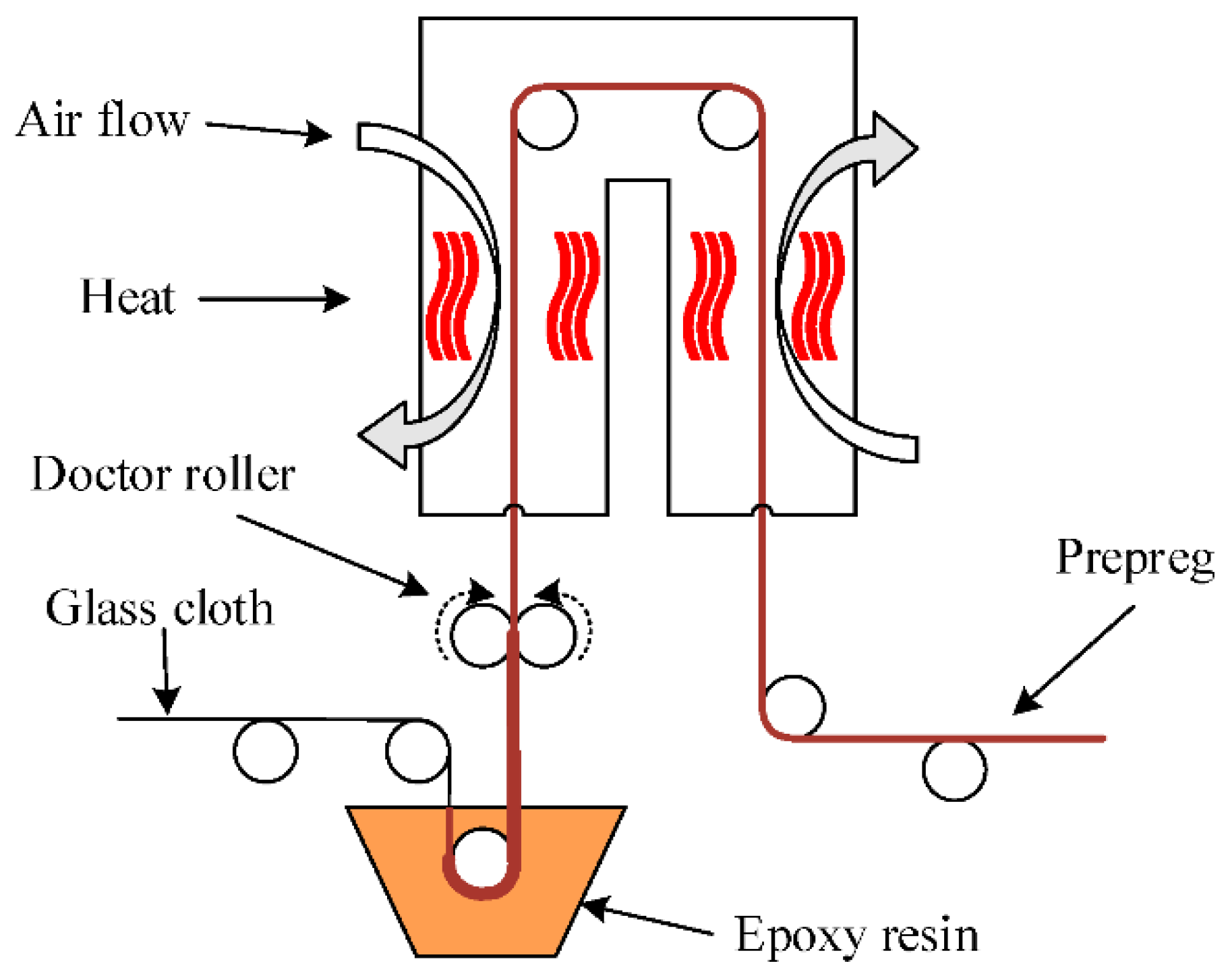
Prepreg is produced by impregnating glass cloth with the epoxy resin. The prepreg can be further laminated with multi prepregs or copper foil to form the base material or CCL. The manufacturing process of the prepreg is illustrated by
Figure 1.
In
Figure 1, the glass cloth is transferred from the left hand side by rollers. First, the glass cloth was impregnated with epoxy resin. Excess epoxy resin which attached to the glass cloth was then removed by two doctor rollers. The rolling direction of the two doctor rollers was opposite to the direction of motion of the glass cloth. Then the glass cloth, with the appropriate volume of epoxy resin, was transferred into a huge oven. In the oven, the epoxy resin was heated and dried. The prepreg was finally complete and was transferred out of the oven.
There are a lot of important parameters for the prepreg manufacturing process. When different prepregs are produced successively in the same machine, setup time is required. Several parameters, including the temperatures of ovens, density of the epoxy resin, and gel time of the epoxy resin, are not easy to adjust and they are always changed while the machine is running. Therefore, the engineers have to adjust the other parameters based on the current temperature of the oven, density of the epoxy resin, and gel time of the epoxy resin, basing their judgments on their experience. Once the new parameters are set, a pilot run is required to ensure the quality of the prepregs. Two quality characteristics, ratio of resin and gel time, were taken into consideration in this research. If the prepregs did not meet the quality requirements, then the parameters needed to be adjusted again. Thus the setup time was increased and the efficiency reduced.
It would be helpful if a prediction model could be built for predicting the performance of quality characteristics of the following lot of prepreg. The concept can be viewed as virtual metrology (VM). VM aims to predict the performance indicators by using parameters such as process variables and machine sensor data, and reduces the usage of physical measurement [
1]. However, VM only provides the quality characteristics based on the given manufacturing parameters. Even with a VM model, the engineers need to know how to adjust the current parameters and make sure that the quality characteristics can be satisfied. Therefore, an optimization methodology for parameter adjustment is also required.
In this research, a dataset of the prepreg manufacturing process was collected. Then the prediction models of VM were developed by support vector regression (SVR) and lasso regression (LR). Finally, mathematical models which integrate the corresponding VM models were proposed to optimize the parameter adjustment.
2. Literature Review
According to the survey of VM for this research, the application in CCL is rarely found in the literature. Kim et al. [
2] proposes the application of virtual metrology for CCL manufacturing to predict product quality derived from processing data without a product quality inspection. Four prediction methods, linear regression, random forest (RF), neural network (NN), and support vector regression (SVR), were adopted with three dimensional reduction methods, namely forward selection (FS), backward elimination (BE), and genetic algorithm (GA). Therefore, the authors developed 12 prediction models. The input variables included temperature, velocity, weight, pressure, and tension measured by sensors, as well as manufacturing variables obtained from the opinions of domain experts. Three output variables, treated weight, minimum viscosity, and gel time, were used. The results show that RF-GA and SVR-GA are more accurate.
VM has been widely applied in semiconductor and thin film transistor-liquid crystal display (TFT-LCD) manufacturing systems. Jonathan and Cheng [
3] dealt with chemical vapor deposition (CVD) machines in a 300-mm semiconductor factory. A back-propagation neural network (BPNN) was developed to predict film thickness. Experimental results show that the maximum error was 1.7%. Hung et al. [
4] dealt with CVD thickness prediction in semiconductor manufacturing. The radial basis function network (RBFN) was adopted to develop the prediction model. Meanwhile, the model parameter coordinator (MPC), which can adjust the values of certain parameters of the VM model to minimize the prediction errors when equipment properties change or different equipment is used, and auto-adjusting mechanism, which can be activated to tune the VM model when the errors between VM and actual metrology values are out of specification, were developed for a real application. The comparison results show that running MPC and auto-adjusting mechanism can further increase the accuracy. Kang et al. [
5] dealt with two etching processes in a Korean semiconductor manufacturing company. Linear regression, K-nearest neighbor regression (KNN), regression tree (TR), NN, and SVR were used to develop a prediction model for VM. Meanwhile, the stepwise linear regression and genetic algorithm with support vector regression were employed for the variable selection method, and principal component analysis (PCA) and kernel PCA (KPCA) were employed as variable extraction methods. The experimental results show that linear regression and SVR are the best prediction algorithms for different quality characteristics. Lin et al. [
6] developed NN as a prediction mode. A stepwise selection method including forward selection and backward elimination was proposed to select a near-optimal set of variables for achieving high VM conjecture accuracy. Based on a piece of semiconductor equipment for the etching process, the results show that the accuracy of NN is better than multi-regression (MR), but the process time will be the issue for real applications. Zeng and Spans [
7] dealt with plasma etching operations and proposed a VM modeling sequence including data preprocessing, outlier removal, variable selection, accommodation of process dynamics, and modeling. In the modeling step, principal component regression, PLS, and BPNN were adopted, respectively. The best result is from a model using BPNN. Lynn et al. [
8] developed global and local VM models for a plasma etching process by using PLS, NN, and Gaussian process regression (GPR). The global models were developed by using all available training points to learn the behavior of a system, and local models were trained using subsets of the available data. The results show that the local model with GPR modeling produces the best estimation accuracy of etch rate on the dataset investigated. Susto et al. [
9] adopted LR and ridge regression for developing the VM prediction model base on a dataset collected from CVD, thermal oxidation, coating, and lithography process. The VM target is a particular quality performance after lithography. The results show that ridge regression outperforms LR in most cases for the dataset used. Kang et al. [
10] proposed a semi-supervised support vector regression (SS-SVR) method based on self-training. A semiconductor manufacturing dataset was collected from the photo process of a South Korean semiconductor manufacturing company. The experimental results show that the proposed SS-SVR method demonstrated excellent performance for a real world semiconductor manufacturing dataset. Jia et al. [
11] proposed an adaptive methodology based on the group method of data handling (GMDH) type polynomial neural networks for predicting the material removal rate for the chemical-mechanical planarization process in semiconductor fabrication. The validation results report improved accuracy in comparison with several candidate methods.
Some VM-related research deals with applications in TFT-LCD. Su et al. [
12] proposed a novel quality prognostics scheme (QPS) for plasma sputtering in TFT-LCD manufacturing processes. The QPS consists of a conjecture model which can estimate the current-lot quality based on the current lot processing parameters and a prediction model which can predict the quality of the next lot according to the current lot conjecture value and the quality measurement data of several previous lots. NN and weighted moving average algorithms were applied to construct the QPS. The test results show that the QPS can be feasible and can conjecture/predict the product quality efficiently and effectively. Su et al. [
13] evaluated various VM algorithms, including BPNN, simple recurrent neural networks (SRNN), and MR. According to the test in fifth generation TFT-LCD chemical–vapor deposition processes, the results show that both one-hidden-layered BPNN and SRNN VM algorithms achieve acceptable conjecture accuracy and meet the real-time requirements. Cheng et al. [
14] defined the VM automation level, proposed the concept of automatic virtual metrology (AVM), and developed an AVM system which has been successfully deployed in a fifth-generation TFT-LCD factory in Chi Mei Optoelectronics (CMO), Taiwan. Hung et al. [
15] proposed an AVMS architecture which can be a useful reference for TFT-LCD manufacturing companies.
In addition to semiconductor and TFT-LCD manufacturing, applications of VM in other industries can be found in the literature. Yang et al. [
16] proposed an approach to apply the AVM system factory-wide in wheel machining automation to achieve the total inspection of all the precision items of wheel machining automation in a mass production environment. Yang et al. [
17] applied VM for inspecting machining precision of machine tools. The test results of machining standard workpieces and cellphone shells of two three-axis CNC machines show that the proposed approach of applying VM to accomplish total precision inspection of machine tools is promising. Hsieh et al. [
18] proposed a scheme to apply AVM for carbon-fiber manufacturing to achieve online and real-time total inspection. Nguyen et al. [
19] developed a novel co-training technique, namely partial Bayesian co-training (PBCT) for a particular semi-supervised learning problem. PBCT was validated on three industrial applications: Gun-drilling, inkjet printing, and low-noise amplifier. The experimental results show that under a reduction of labeled data by up to 50%, a robust estimation is still attainable.
The problem that the present study addresses was not found in the literature. The review of the literature shows that VM has been studied in some industrial settings, including CCL, but the further application of integrating with parameter adjustment, which can provide an opportunity to reduce the number of setups or setup time, is not found in the literature. Consequently, the proposed VM based parameter adjustment optimization may be of benefit in many similar industries.
4. Parameter Adjustment Optimization
In the prepreg manufacturing process, there are two important output variables: The ratio of resin and gel time. This research adopted the prediction tools to develop VM models for both output variables, respectively. Moreover, parameters such as temperatures of ovens and density of epoxy resin are not easy to adjust, and engineers always want to minimize the adjustment of these parameters, and adjust other parameters. Based on both VM models, this research aimed to minimize the sum of adjustments to all parameters. A mathematical model was developed for optimizing parameter adjustment and the required notation is defined as follows:
: current value of input variable j;
: Suggested input variable j;
: The normalized adjustment amounts of input variable j;
: The value of input variable j of instance i;
: Normalized deviation value of output variable k;
: Target value of output variable k;
: Lower control limit of output variable k;
: Upper control limit of output variable k;
H: Set of input variables which are hard to be adjusted.
The mathematical model aimed to minimize the sum of normalization of deviation between output values and their corresponding target values as given in Equation (10). In Equation (11),
indicates the VM model of output variable
k, and
is the corresponding VM value output value
k. As the scales of output variables are quite different, this research normalized the deviation between output values and their corresponding target values by Equation (12). Equation (13) specifies the bounds of input variables. Equation (14) indicates that the input variables which are hard to adjust have to retain their current value.
5. Experimental Results
5.1. Data Description
This research used real-world data collected from the prepreg manufacturing department of a plastic company in Taiwan. The demand for different products varies widely in the company. For the products with high demand, as the manufacturing data has been studied for a long time, the engineers can adjust input values very well in the light of their experience. Moreover, these high demand products are always assigned to specific production lines. Thus the number of setups can be reduced and increase the efficiency of these production lines. There are many different types of products with low demand, but the corresponding manufacturing data is relatively sparse. Therefore, engineers lack experience in setting up these product types. These low demand products are also assigned to specific production lines. The both number of setups and setup time are very high, and this reduces efficiency of these production lines. This research focuses on one production line which always produces low demand product types.
The collected input and output variables are listed in
Table 1. There are 12 input variables and 2 output variables. Among input variables, moving speed is the transfer speed of the glass cloth, which affects the heating time in the oven. Epoxy resin density is the density of resin which is the raw material of the impregnation process. There were two oven temperatures, as shown in
Figure 1; one was the temperature of the oven on the left-hand side and the other was the temperature of the oven on the right-hand side. There were two doctor rollers, the positions of which affected the volume of resin that adhered to the glass cloth. Moreover, there were four fan speeds, as shown in
Figure 1. The first was located on the upper left for moving air into the oven, the second was located on the lower left for moving air out of the oven, the third was located on the upper right for moving air out of the oven, and the fourth was located on the lower right for moving air into the oven. Revolution speed was the revolution speed of both doctor rollers. Gel time 1 indicated the gel time of the epoxy resin. It was the time required for resin to become solid at a certain temperature.
It can be noted that among input variables, epoxy resin density, oven temperature 1, oven temperature 2, and gel time 1 were hard to adjust. Epoxy resin density and gel time 1 were the attributes of the epoxy resin, and the epoxy resin was made before it been put into the trough. Therefore, it was impossible to adjust epoxy resin density and gel time 1. Both oven temperatures were increased by electric energy and cost was required, but both oven temperatures were reduced by itself and time was required. Therefore, engineers always want the temperature stay the same.
Regarding the output variables, the ratio of resin was the ratio of resin weight in prepreg, and gel time 2 indicated the gel time of the resin in prepregs.
All instruments were well integrated, and almost input variables could be monitored and controlled by a central control system. However, epoxy resin density, gel time 1, ratio of resin, and gel time 2 could only be measured by manual labors. Every time when new parameters were set, the four variables were entered into the system manually. Moreover, all of the instruments were calibrated regularly. This research collected the manufacturing data of a production line which focuses on producing low demand products. The products which are produced by a certain type of glass cloth and a certain formula of epoxy resin were collected. From January 2018 to January 2019, 216 sets manufacturing data were collected. The maximal and minimal values of all input and out variables are shown in
Table 1. Although the collected 216 sets of data were based on a single production line, type of glass cloth, and formula of epoxy resin, the corresponding specifications were quite different because they respond to customer needs. Consequently, the target values of the collected data were not the same.
According to preliminary tests, there was an obvious relationship between the square and interaction of input variables and output variables. This research also analyzed second order terms of all input variables. This meant that the 12 input variables produced 90 terms (12 original variables, 12 squares of variables, and 66 interactions between variables).
5.2. VM Model Development
Based on the collected data, 66.7% of data were randomly selected for training and the remaining 33.3% were saved for testing. According to the introduction in
Section 3,
λ and
C were important parameters for LR and SVR, respectively. This research adopted 10-fold cross-validation to evaluate the trained VM model with different
λ or
C. That means the training data was divided into 10 parts. For each
λ or
C, one model was developed based on 9 parts, and validated by the remaining part. Following the same procedure, 10 models were developed and then validated. The level of
λ or
C with the lowest average mean absolute percentage error (MAPE) of the 10 validations was then adopted for training the VM model with all the training data.
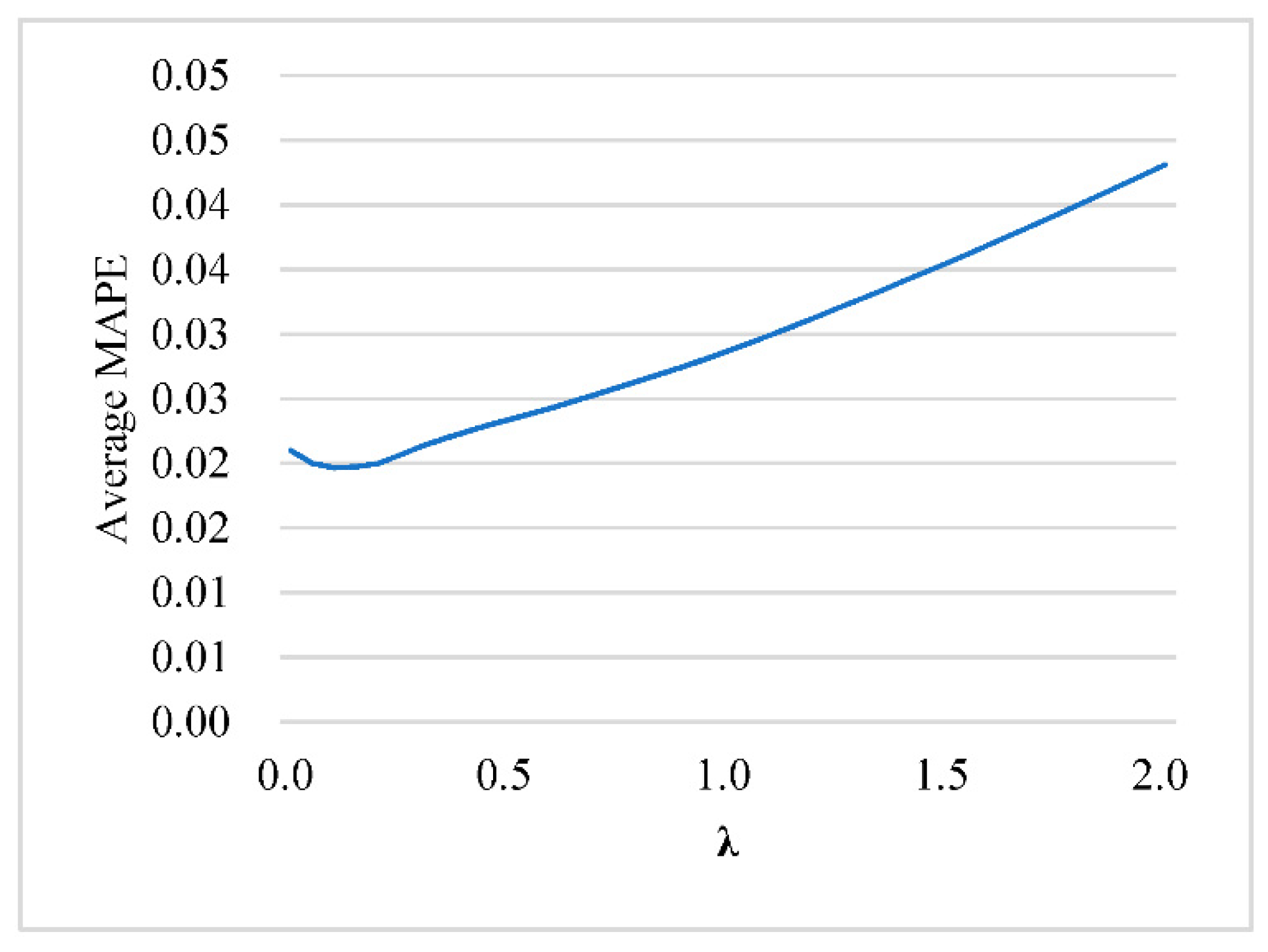
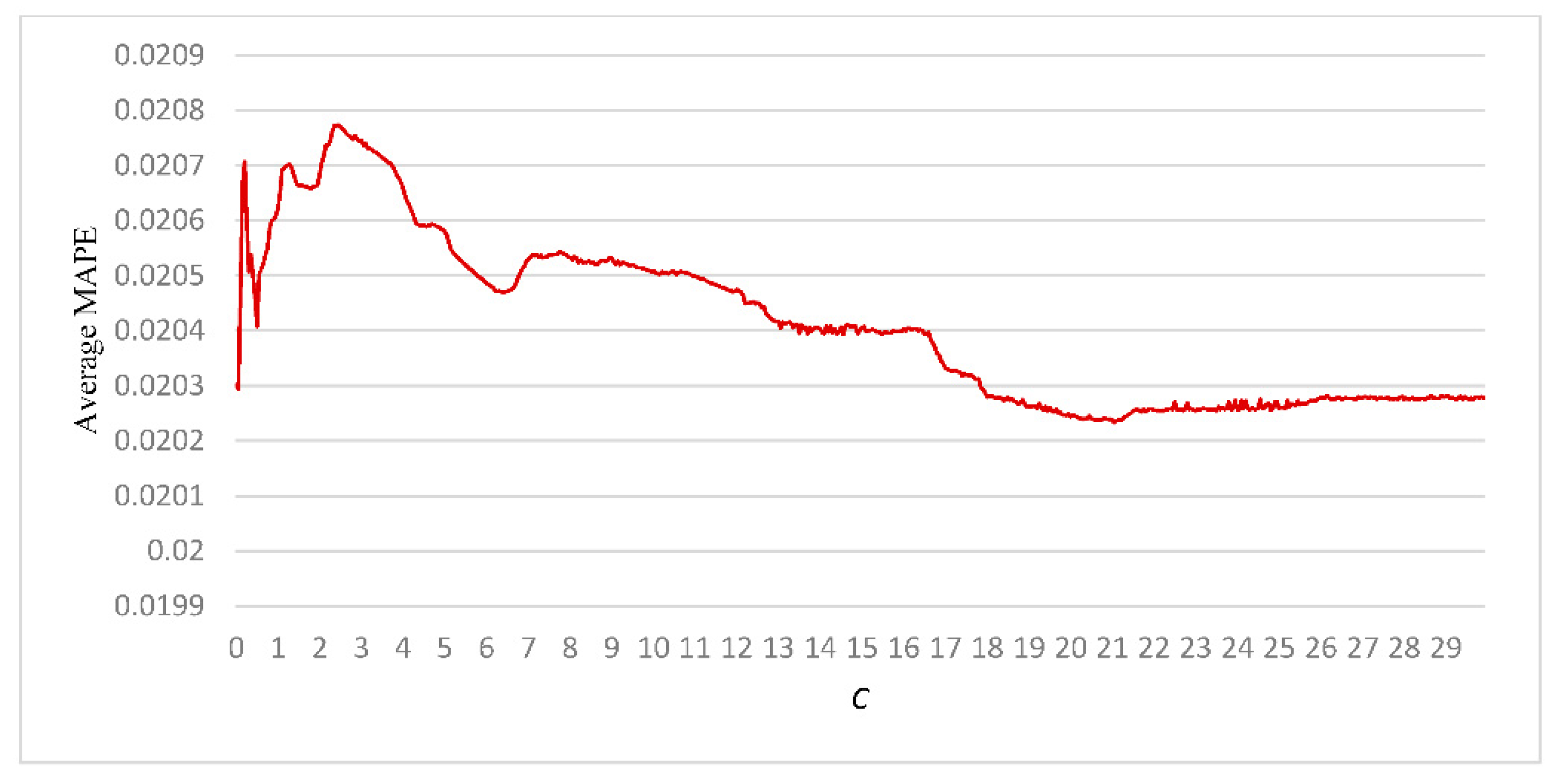
In this research, LR was trained based on
λ between 0 to 2, and SVR was trained for
C between 0 to 30. The training results of LR and SVR for the output value “ratio of resin” are illustrated in
Figure 3 and
Figure 4. When
λ = 0.1 and
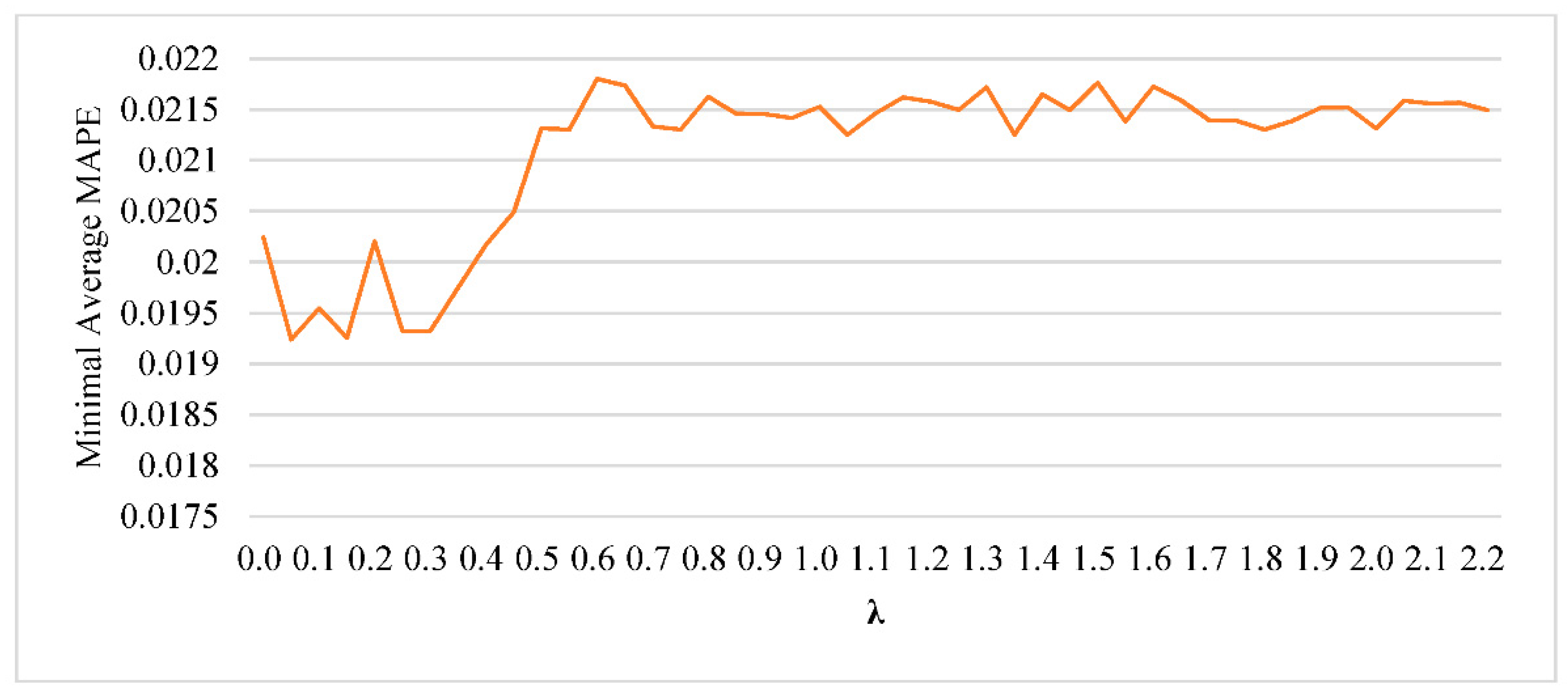
C = 21.1 the average MAPE of the corresponding trained LR and SVR were the lowest. Regarding LR+SVR, both
λ and
C needed to be optimized. A full factor experiment was constructed, and the results for output value “ratio of resin” are illustrated in
Figure 5. In
Figure 5, only the lowest average MAPE of each level of
λ are shown. When
λ = 0.05 the average MAPE was the lowest with
C = 1.75. The final training and testing results are shown in
Table 2.
Table 2 shows the performance of the six developed VM models. It was found that using LR+SVR and taking second order terms into consideration had the best performance in training and testing results for both output variables. This research then adopted the two developed VM models for optimizing the adjustment of input variables.
5.3. Optimizing Adjustment of Input Variables
Once the VM models were developed, the mathematical model proposed in
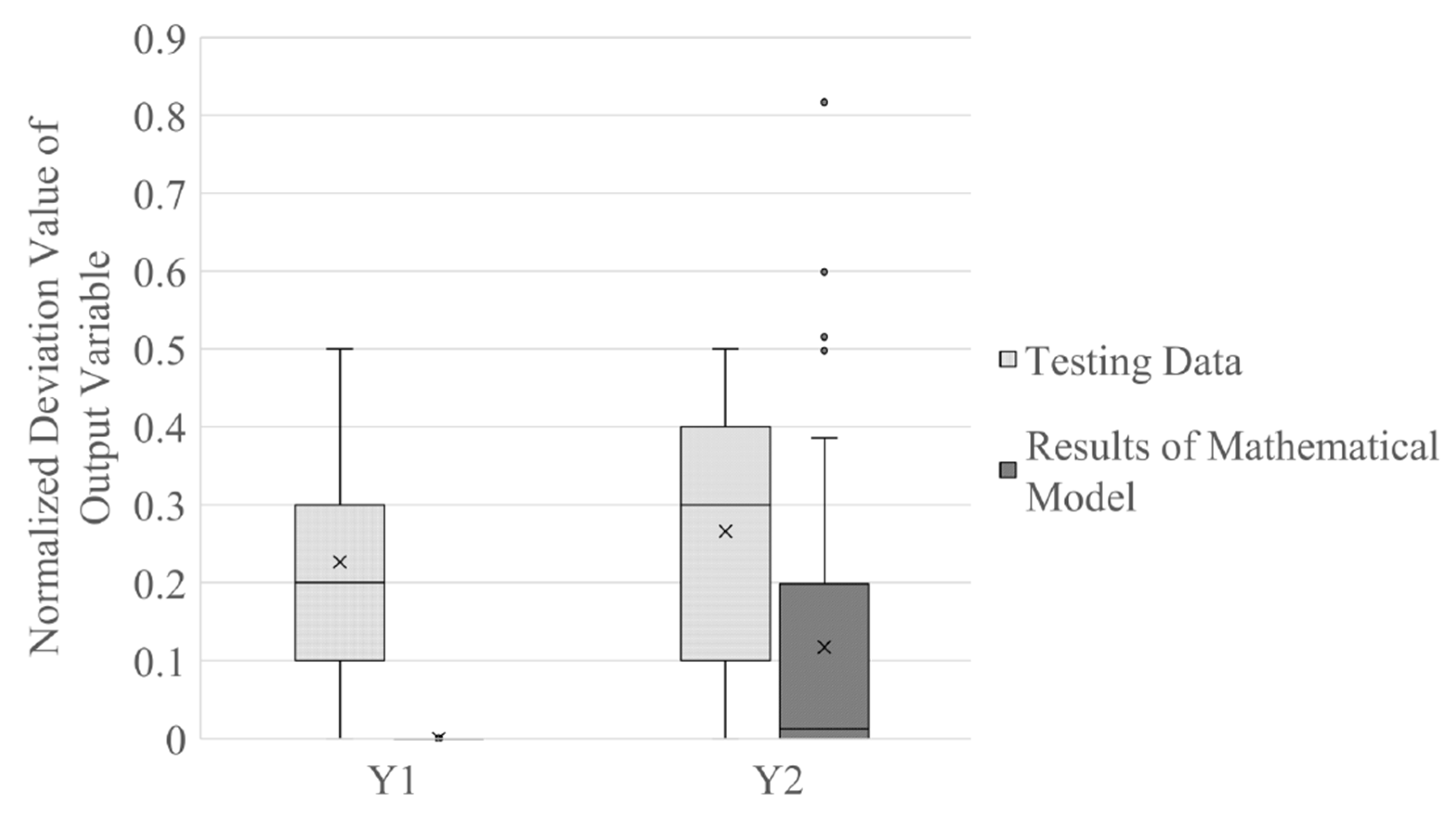
Section 4 could be adopted to optimize adjustment of input variables. This research tested the mathematical model on the 33.3% of test data using the software Excel Solver. The average normalized deviation of output variables for ratio of resin and gel time 2 with the test data were 0.227 and 0.266, respectively. Based on the adjustment using the results of the mathematical model, the average normalized deviation of output variables for ratio of resin and gel time 2 in the test data were 5.642 × 10
−6 and 0.117, respectively. The results are summarized in
Figure 6 by box plots.
On average, the proposed mathematical model provided better input variables which can produce output variables that are closer to target values. However, as shown in
Figure 6, the proposed mathematical model produced results for output variables of gel time 2 that were far from the target values in some test data. This research then modified the mathematical model proposed in
Section 4. Firstly, in order to minimize the deviation of output variables, Equation (15) was added to ensure that the resulting output variables were equal to the target variables. Thus, Equation (12) is redundant in the modified model.
Then the objective function was replaced by Equation (16), in order to minimize the normalization of adjustment of all input variables. As the scales of input variables were quite different, this research normalized the adjustment of input variables by adding Equation (17).
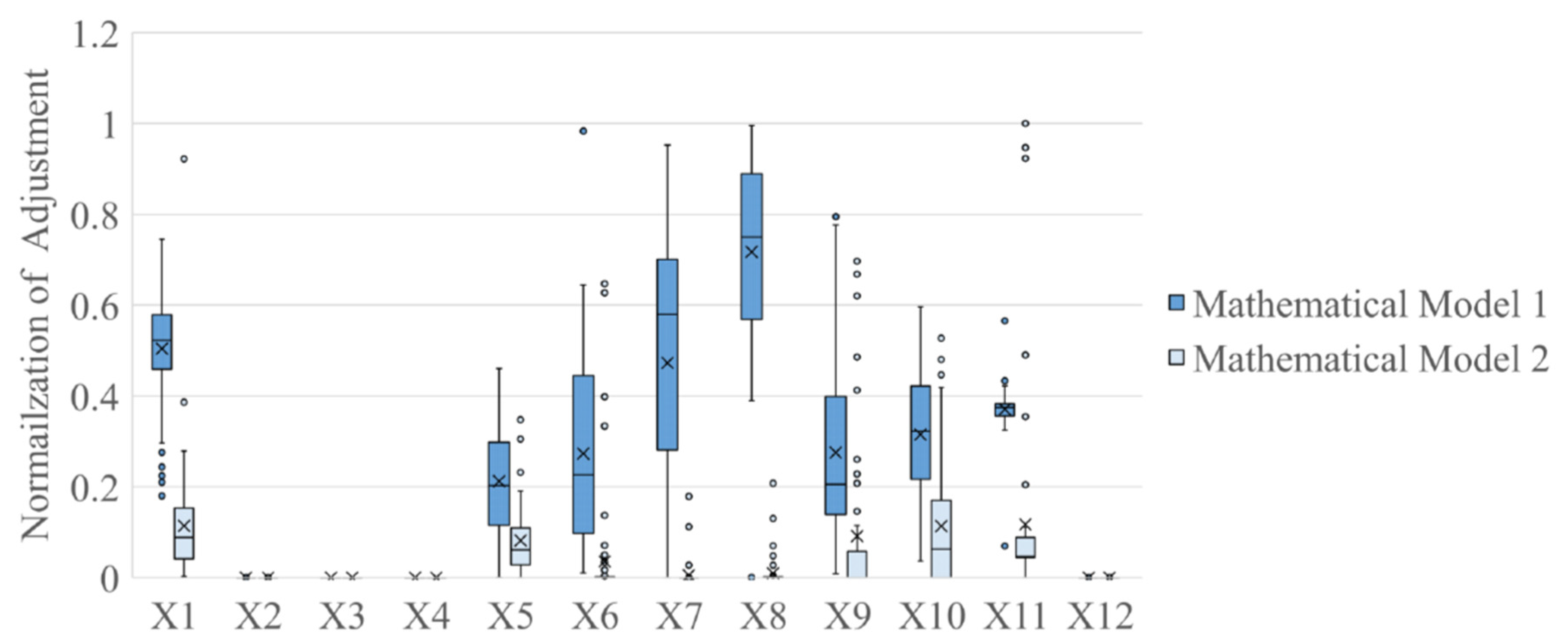
From Equation (16), the deviation of output variables of the modified mathematical model was reduced to zero. The results for the adjustment of input variables were illustrated in
Figure 7. In
Figure 7, the mathematical model proposed in
Section 4 is called mathematical model 1, and the mathematical model modified in this section is called mathematical model 2. In
Figure 7, input variables
X2,
X3,
X4, and
X12 were hard to adjust, and their corresponding adjustment for all instances was very close to zero. Moreover, the average adjustment of input variables produced by mathematical model 2 were smaller than those of mathematical model 1; although, in rare instances, the adjustments of input variables
X1 and
X11 produced by mathematical model 2 were bigger. Mathematical model 2 was more robust in providing values of input variables with less adjustment.


