Comparing Classical and Modern Machine Learning Techniques for Monitoring Pedestrian Workers in Top-View Construction Site Video Sequences

Abstract

Keeping an overview of all ongoing processes on construction sites is almost unfeasible, especially for the construction workers executing their tasks. It is difficult for workers to concentrate on their work while paying attention to other processes. If their workflows in hazardous areas do not run properly, this can lead to dangerous accidents. Tracking pedestrian workers could improve the productivity and safety management on construction sites. For this, vision-based tracking approaches are suitable, but the training and evaluation of such a system requires a large amount of data originating from construction sites. These are rarely available, which complicates deep learning approaches. Thus, we use a small generic dataset and juxtapose a deep learning detector with an approach based on classical machine learning techniques. We identify workers using a YOLOv3 detector and compare its performance with an approach based on a soft cascaded classifier. Afterwards, tracking is done by a Kalman filter. In our experiments, the classical approach outperforms YOLOv3 on the detection task given a small training dataset. However, the Kalman filter is sufficiently robust to compensate for the drawbacks of YOLOv3. We found that both approaches generally yield a satisfying tracking performances but feature different characteristics.

1. Introduction

Construction sites constitute highly dynamic environments in which workers execute diverse orders simultaneously. Workers need to perform tasks, interact with heavy construction equipment and keep an eye on their surroundings, which is difficult for complex tasks. This requires construction workers to have a high level of concentration to avoid mistakes. If the construction site is noisy and congested, it can be difficult for the construction workers to concentrate on their work and the environment at the same time. In addition, the continuous change of a construction site often leads to hazardous situations. Heavy construction machines move across the site to execute their jobs. Construction vehicles cross the worker’s paths and cranes lift loads over their heads. In addition, pedestrian workers inevitably share the same workspaces with construction machines or interact with them in order to accomplish their orders [1]. As a result, worker’s activities often happen in close proximity to heavy machinery. Hazardous situations such as close calls can occur as a consequence of this [2]. Furthermore, in certain cases, people can misjudge the danger. Due to the mentioned facts, it is to be expected that workflows on construction sites are not always ideal. In addition, the incidents lead to hazardous situations for pedestrians on construction sites. Thereby, the pedestrian worker can be injured or have a fatal accident. For these reasons, construction workers undergo regular training to raise their awareness with respect to hazardous situations [3] as well as to develop their knowledge and skills [4] to improve their workflows. Despite this effort, working in the surroundings of heavy construction machines remains to be a hazardous job. Identifying a reasonable workflow during its execution in a steadily changing environment also keeps to be a challenging concern. Accordingly, productivity and safety problems continue to occur on construction sites.

Monitoring pedestrian workers on the sites from a top-view perspective could improve this situation. This way, the worker’s trajectories could be analyzed and adaptations to their workflows could be made during their work [5]. In addition, a monitoring system would help the machine operators in their work, as they usually do not have a complete overview of the environment [1]. In this case, the positions and movement directions of workers who are nearby could be provided to the machine operators. This would allow them to recognize hazardous situations at an early stage and take appropriate action to prevent an accident. The mentioned scenarios represent possible applications of a monitoring system on construction sites, for which a suitable method has to be investigated. Therefore, in this paper, we only focus on the detection and tracking of construction workers, since this is the basis for a surveillance system.

Different approaches have already been made in tracking pedestrian workers on construction sites. Depending on the surrounding, various technologies are used for monitoring workers in construction related scenarios [6]. The literature often refers to global navigation satellite system (GNSS) tags for outdoor localization on construction sites [7,8]. This is mainly applied to track construction machines and equipment, but some approaches make use of GNSS to locate pedestrians on site [9,10]. Near buildings, walls or large construction elements, GNSS-based localization is affected by multipath effects caused by reflections of the signal on these objects [11,12]. Since construction workers often work near these objects, tracking such workers with GNSS becomes unreliable. Less sensitive approaches rely on radio-frequency technologies. These also include the attachment of tags to the worker’s gear. Corresponding readers can either be stationary on the construction site or attached to construction machinery. Employing a setup that utilizes radio-frequency identification (RFID) technology enables the warning of workers and machine operators whenever a tagged worker gets into the range of a machine’s reader [13] or specific zones [14]. Other approaches develop systems noticing pedestrian workers when entering certain zones by localizing them using ultra-wideband (UWB) tags [7]. Although the accuracy can be improved by combining RFID technology with ultrasound [15], a precise localization and tracking of workers in real time constitutes a challenging task [7] which has not been sufficiently solved in general yet [16]. Besides technical deficiencies, the deployment of such a system for the implementation of a tracking application on a real construction site requires a tag for each worker. Additionally, at least three receivers per monitored area have to be installed in the case of two-dimensional tracking which results in high acquisition costs [6]. Furthermore, workers perceive the attachment of tags with unique identifiers (IDs) to their gear to be obtrusive and to cause discomfort [17].

In contrast to tag-based methods, camera-based tracking approaches provide cost-effective surveillance alternatives. The costs amount to one camera per monitored area and there are no further costs for additional equipment for the workers. In research, some effort has already been made to detect construction worker’s in camera images [18]. Park and Brilakis [8] built a real-time capable detection scheme to recognize construction workers in camera images for initializing a visual tracker. They used background subtraction via a median filter to find moving objects within the images. Then, a pedestrian detection is performed on these objects using a support vector machine (SVM) which operates on Histogram of Oriented Gradients (HOG) features. Exploiting the loud colors of the worker’s safety vests, construction workers are identified from the pedestrian detections by clustering hue, saturation, value (HSV) color histograms using a k-Nearest Neighbors (k-NN) algorithm. Chi and Caladas [19] also decided on background subtraction to identify moving objects before classifying these by a neural network approach. In [20], the background subtraction is exchanged by a sliding window approach. However, similar to Park and Brilakis [8], they used HOG and color features but concatenate them to a single vector which is passed to a SVM in order to identify workers. Using color and spatial models classified by a Gaussian kernel, Yang et al. [21] decided on a similar strategy. In recent years, deep neural network based approaches have become prominent. To recognize worker’s activities, Luo et al. [22] applied temporal segment networks. Son et al. [23] used an region based convolutional neural network (R-CNN) based on ResNet to detect workers under changing conditions. Luo et al. [24] proposed an approach which detects construction workers in oblique images of cameras mounted in heights. They applied YOLO for detection but only achieved a precision of about 75%. Vierling et al. [25] proposed a convolutional neural network (CNN)-based concept detecting workers in top-view images. To cope with high altitudes, their approach relies on several zoom levels each with a separate CNN for detection. An additional meta CNN is used to choose the correct zoom level for a certain height.

Despite the use of transfer learning techniques, CNN-based approaches usually require large amounts of training data. Corresponding data, which represent construction sites from a top view perspective, are rarely available. In addition, the generation of a sufficiently large dataset is a time-consuming and demanding task. Beyond that, these networks commonly operate on small image sizes of about 400 × 400 px. High resolution images cannot be processed in real time without disproportionately large amounts of computational power or without drastically downscaling images. Since surveillance cameras monitor large areas of construction sites, workers occupy only very small parts of the image. Besides the fact that detecting small objects with CNNs is a challenge, reducing the size of the image makes detection even more difficult. The downscaling may eliminate relevant features in the image required for a reasonable detection.

As it is unclear whether CNNs can outperform classical machine learning methods on these terms, we conduct a comparison in this paper. The goal of the comparison is to find out whether one of the two approaches can satisfactorily track several construction workers when the amount of training data is small. In doing so, we restrict our focus to one view within one construction site at first. In this case, a camera could be mounted, e.g., on the mast of a tower crane. Alternatively, several cameras could be used to completely monitor a construction site, but this is not covered in this paper. Because no suitable dataset is publicly available for comparison, we assemble a small generic dataset ourselves. This shows pedestrian construction workers from a top view perspective under different conditions. As a representative CNN approach, we choose YOLOv3 [26], since it is a state-of-the-art detection network. For its counterpart from the field of classical machine learning, we rely on preliminary work [27] discussing diverse computer vision techniques for monitoring construction workers. In this work, we juxtapose eligible methods and develop a theoretical concept relying on a classical machine learning method. Based on these results, we implement a tracking approach based on a soft cascaded classifier in the course of this paper. A simple Kalman filter is applied to both approaches in order to track the detected workers within the recorded video sequence. In our experiments, we compared the detection and tracking results of our implemented approach with those of YOLOv3 trained on the same data. We found that our classical machine learning approach yields substantial better detection results on the small dataset than the CNN. However, the Kalman filter proves to be sufficiently robust to compensate for the lower detection quality of YOLOv3. Owing to this, both approaches perform similarly well on the tracking of pedestrian workers in general. Nevertheless, each approach possesses different tracking characteristics. A general recommendation can, thus, not be made. The appropriate tracking solution has to be determined with respect to the demands of the particular application.

2. Materials and Methods

To compare the performance of CNN-based and classical computer vision approaches to the monitoring of pedestrian workers, we assembled a small characteristic dataset. This dataset includes different scenarios as well as various environmental conditions. Section 2.1 describes the dataset in detail. This dataset is used for the training and the evaluation of both approaches chosen for our comparison. The classical approach is composed of a soft cascaded classifier and a background subtraction which preprocesses the input images to enable detection in real-time. Its detailed structure and the parameter optimization are described in Section 2.2. YOLOv3 also possesses several hyperparameters. In Section 2.3, we elaborate on our choice of those hyperparameters. For a better comparison, the detections of both approaches are tracked by the same method over the course of the video sequences. We chose Kalman filtering for this as it is a simple but robust method which is sufficient for the purpose of comparing the two approaches. Details about the Kalman filter’s motion model and other required parameters are given in Section 2.4. The implementation and testing of the two approaches was done with the programming language C++ on a standard computer.

2.1. Dataset Acquisition

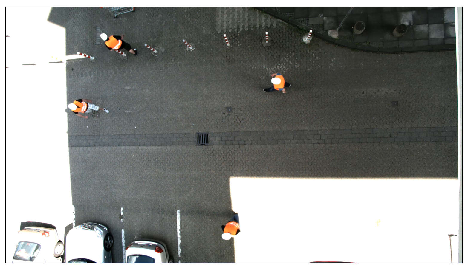
Top-view scenes of construction sites have rarely been recorded. Accordingly, a dataset reasonable for our purpose has not been published yet. For that reason, we recorded video sequences to train and test our approach explicitly for the scope of this paper. It is important to know if different backgrounds and lighting conditions can have an influence on the tracking of construction workers. In addition, we want to test if our approach can distinguish between different moving objects. The videos were therefore taken in two scenarios with different levels of difficulty for our approach: in the first one, construction workers act on a uniformly plastered terrain, whereas a mixture of gravelled and plastered areas is chosen for the second scenario. While the first scene is illuminated well, the second scene is slightly overexposed. Both sequences are recorded by a non-pivoting camera at a height of 20 $\mathrm{m}$, which is aligned to the ground and has a fixed position (see Figure 1). This results in a top-view perspective in the center of the image, but becomes oblique at the borders of the image. In accordance with a typical crane camera set up [28], all videos were recorded with a frame rate of 25 fps and a resolution of 1920 × 1080 px. In both scenarios, construction workers wearing safety vests and helmets walk randomly through the camera’s field of view including sudden stops and directional changes. They also interact with static construction specific elements such as pylons and barrier tapes. Of course, exposing workers intentionally to hazardous situations or heavy construction machinery is unwarrantable. Such hazardous situations are substituted by smaller moving vehicles instead which still allows for evaluating the correct classification of moving objects. In both video sequences, the construction workers are manually labeled by hand in order to prepare both the ground truth and the training data. Rectangular areas surrounding the worker’s heads and shoulders are used to indicate the positions of the workers.

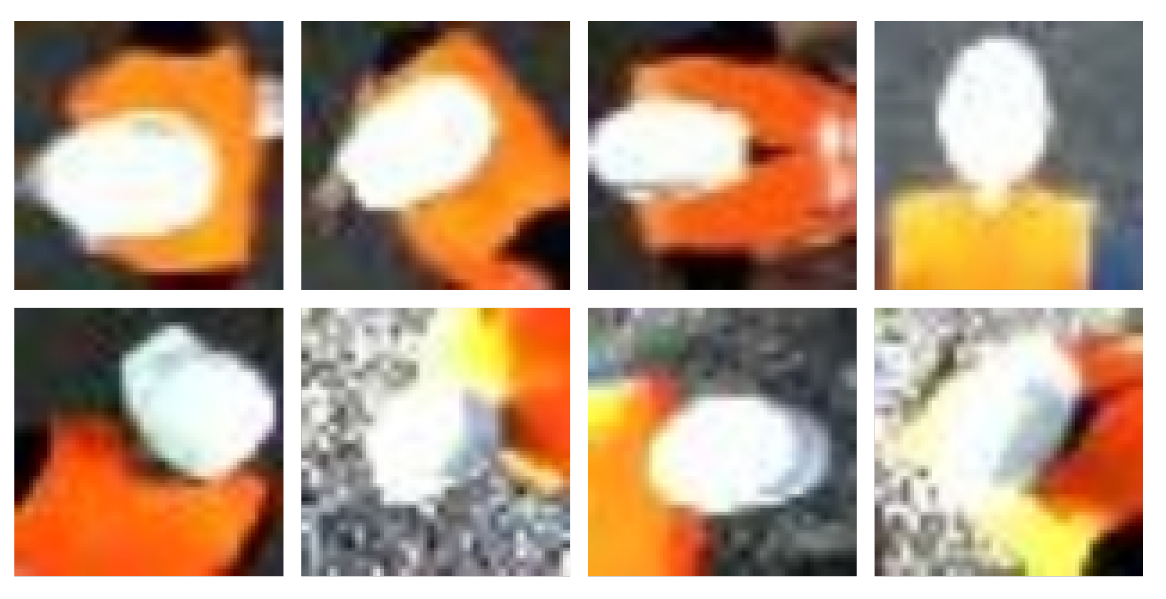
Datasets for training, validation and evaluation are generated from the labeled sequences. For this, we divide each sequence into three shares of equal length. From the first share of both sequences, we generate the training dataset. This training dataset includes 1000 pedestrian construction worker samples (see Figure 2). Samples are only extracted from every 10th frame to reduce the similarity among the samples. For generating the validation dataset, we proceed analogously with the second share of both sequences. The validation dataset also contains 1000 pedestrian construction worker samples. From the third part, we generate evaluation data that consist of video sequences with an average length of 12 s. From each sequence, we choose a representative scene which contains settings commonly occurring on construction sites. Both scenes show up to four pedestrian construction workers simultaneously and other objects colored similarly to the worker’s safety vests that are either static or moving. The static objects are red and white barrier posts, barrier tapes and a red barrier on a gravel area. These elements have similarities to the colors of the construction workers. Moving objects include a red vehicle that moves linearly in the same direction as a construction worker. In addition, the red color between the worn safety vest and the vehicle is similar. The workers walk through the scene while sometimes passing each other closely. In addition to these two scenes, we choose a third one to evaluate our approach with regard to moving vehicles. This scene shows a single worker walking while a car approaches him from behind.

2.2. Classical Detection Approach

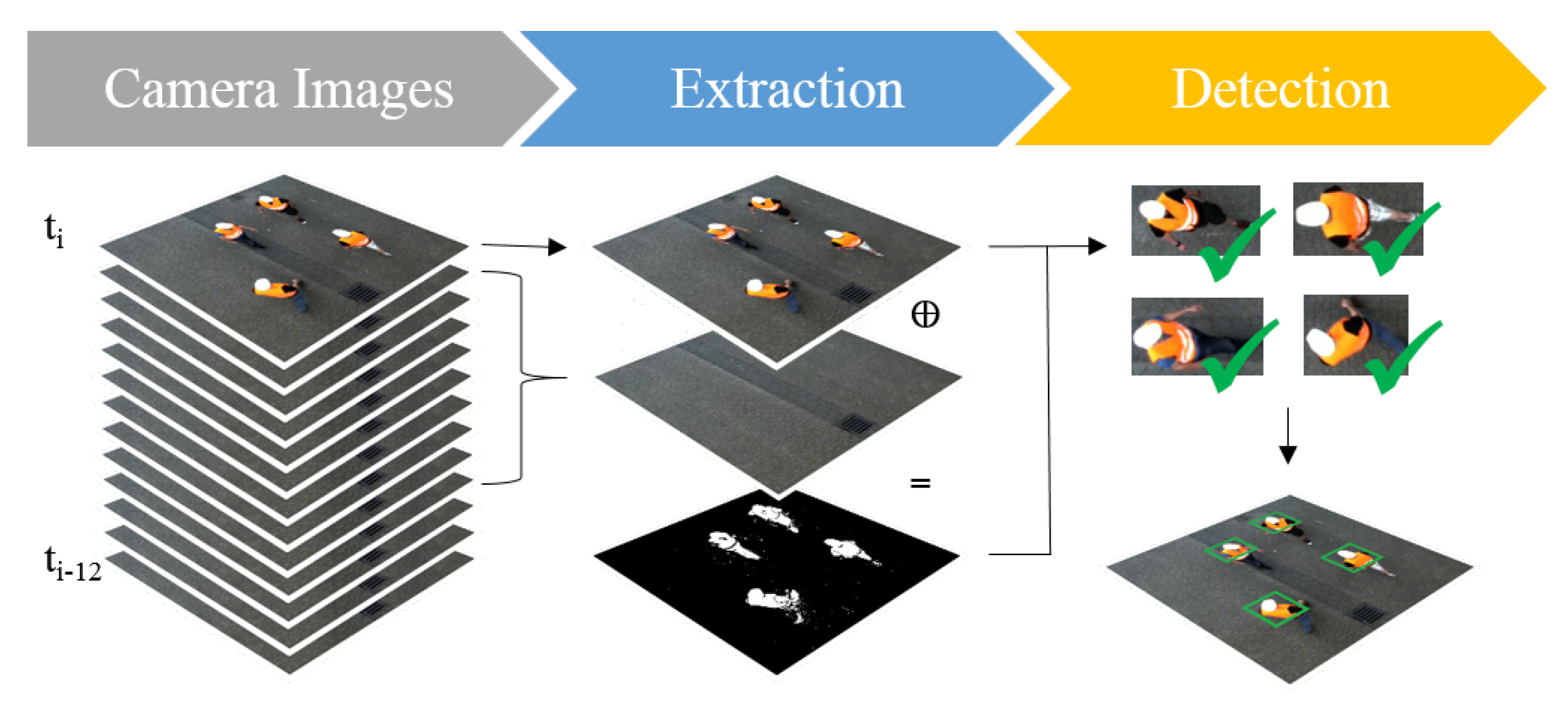
Based on our theoretical concept previously proposed in [27], we implemented an explicit approach to detection of construction workers in top view images. As shown in Figure 3, detection is done by first extracting relevant regions of interest (RoIs) from the current camera image. Afterwards, each region is classified to determine whether it contains a worker or not.

Most previously implemented image-based approaches in civil engineering are based on a frontal camera perspective. In our case, however, the camera is mounted at a height in order to monitor a large area and to satisfy the requirements of different applications. This leads to a top-view perspective. Most features that make up a pedestrian, such as legs and arms, are usually covered by his own body due to the perspective. Although there are already approaches for the general detection of pedestrians in top-view images, detecting pedestrian workers can be eased by leveraging typical features that characterize those workers. On construction sites, workers wear helmets and safety vests with loud colors that constitute clearly visible and prominent features. Similar to the findings of Park and Brilakis [8], a combination of motion, color and shape features is more reasonable for a proper detection in our scenario than the use of common pedestrian detection features. While motion is a fundamental characteristic of pedestrians, it is not unique to them. Other objects such as construction vehicles may also move through the cameras field of view so that classification by motion is unrewarding. Notwithstanding, constraining the detection to image regions containing movement spares the expense of investigating the entire image. This improves the subsequent detection in two different ways. On the one hand, applying the classifier to only a few regions of the image significantly speeds up the detection process which allows for the monitoring of substantially larger areas of a site without an appreciable time lag. On the other hand, this preselection excludes most image regions not containing any construction workers from the further detection process which highly reduces false positive detections in advance.

To find regions of motion, moving foreground objects have to be separated from the background. For this, Gaussian mixture models are frequently used and well established methods estimating a scene’s background are available [8]. We use an improved adaptive Gaussian mixture model (GMM) approach [29], because it is insensitive to background movements that often occur in outdoor scenarios, e.g., wobbling bushes or leaves blown by the wind [30]. To adapt to changes in the scene such as varying illumination conditions or newly positioned and removed static objects, the mixtures of Gaussians are learned and adjusted over time. Accordingly, the Gaussians’ parameters, their number per pixel, as well as the learning rate are updated online by the adaptive approach while applying the model to consecutive video frames.

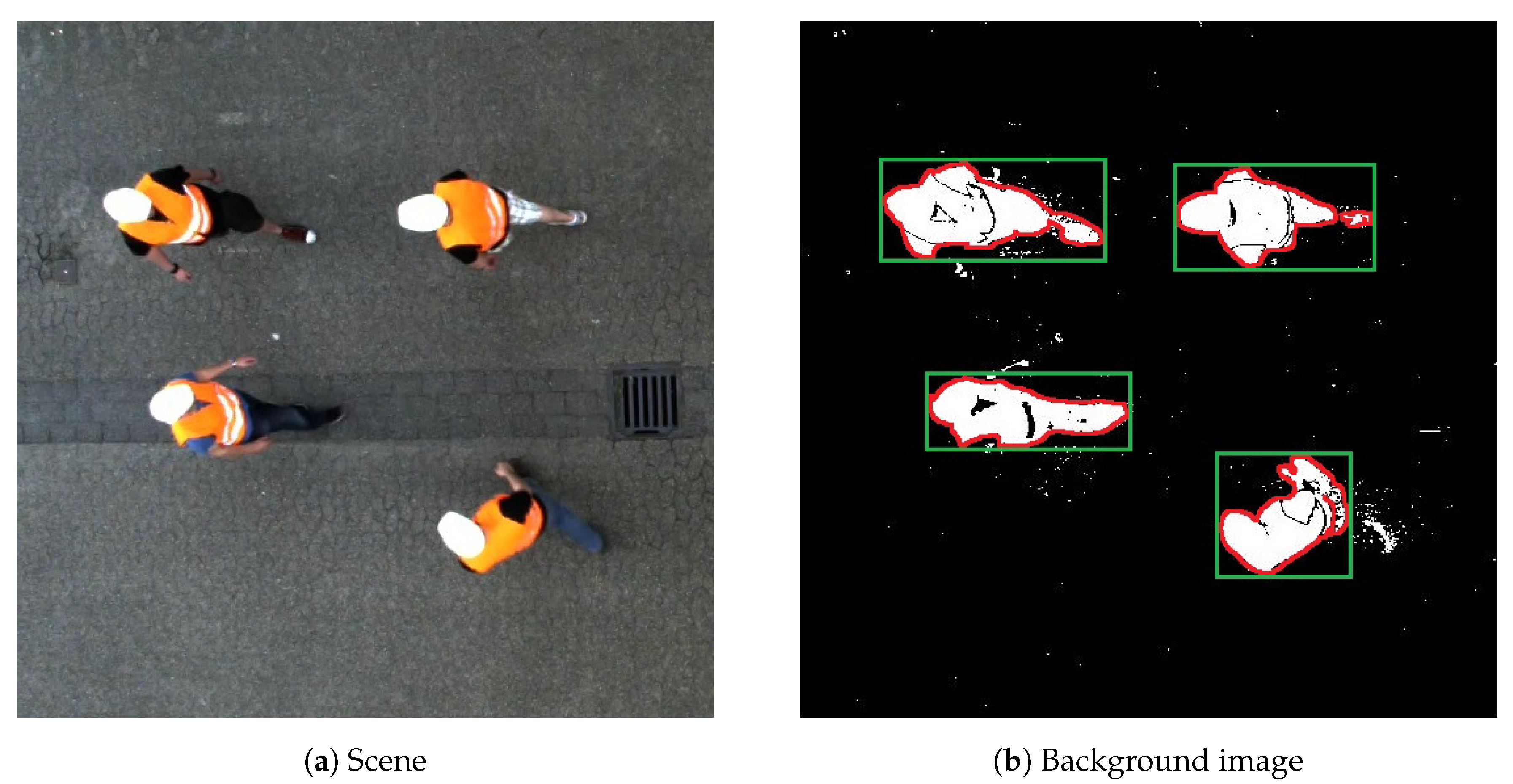
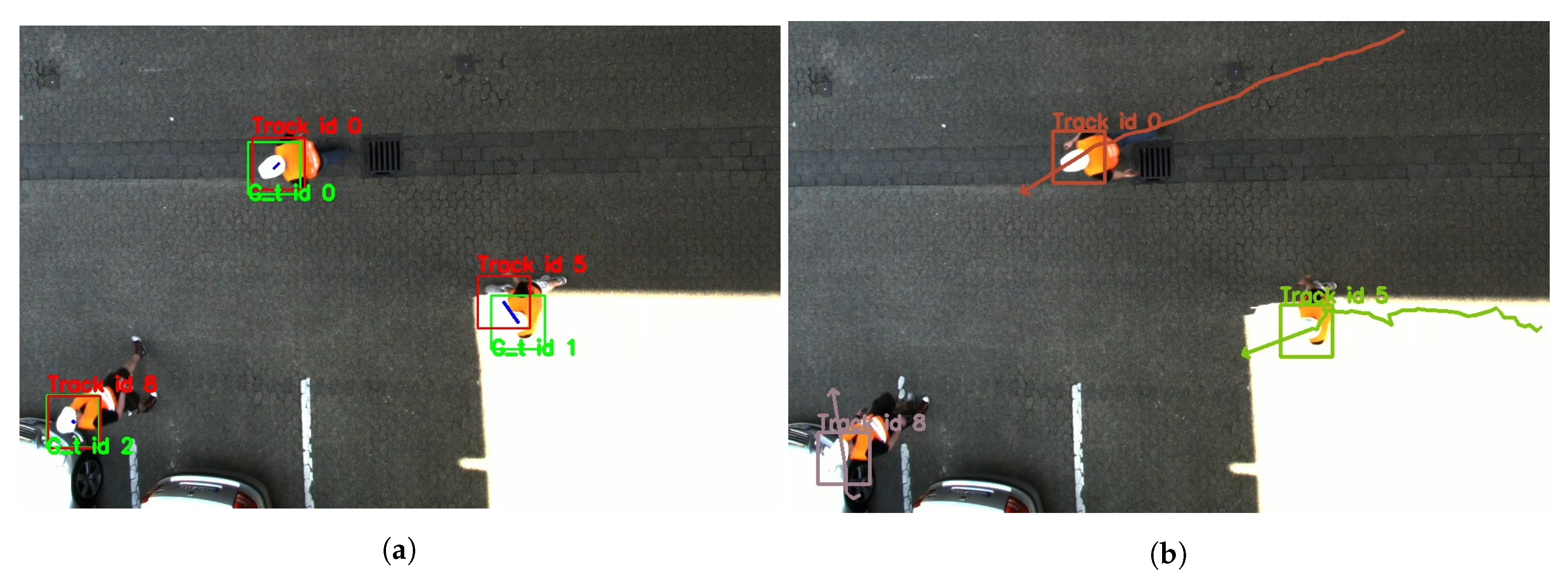
Comparing the current frame (see Figure 4a) to the learned background model results in a binary segmentation image which indicates fore- and background pixels. In the next step, all connected foreground pixels are aggregated to regions of motion by blob detection. For this purpose, an algorithm is used that finds contours in the binary image [31]. In a further step, rectangles are formed, which enclose each contour. These rectangles identify the RoIs for the further detection process, as shown in Figure 4b.

Since the background subtraction identifies the relevant areas within the image which are likely to contain pedestrian construction workers, the detector only has to focus on those image regions. Each of those RoIs contains a single moving object in the scene. Distinguishing between a worker and any other object can be done by a binary classification for each RoI.

As described above, construction workers in top-view images are characterized best by their motion, color and shape. The classification of color and shape features provides a proper basis of decision-making since we already use motion to find candidate regions. Following this, we use color histograms as they are simple but effective color feature descriptors. The histograms are computed on the hue and saturation channels of the HSV color space. Since the value channel decodes brightness, it is neglected in favor of the histograms’ invariance to changes in illumination conditions [8], which is a common issue in outdoor scenes. For determining shape information, we decided on Haar-like features. The choice of these features allows us to design both feature descriptors as low-order integral channel features [32]. This guarantees the efficient computation of the feature responses which increases the detection speed. However, it remains unclear how to arrange those feature descriptors’ positions and sizes on an image patch so that they optimally respond to a construction worker.

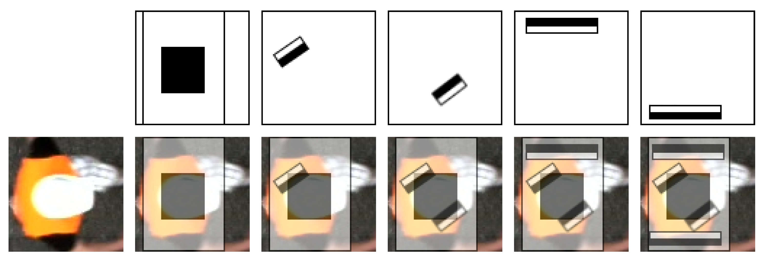
For this reason, we apply a Soft Cascaded Classifier [33] which learns the optimal set of features using AdaBoost [34]. For this, we deduce weak classifiers from the feature descriptors by thresholding their responses. Then, we generate a weak classifier pool containing thresholded feature descriptors at all conceivable sizes and positions in an image patch. During training, AdaBoost iteratively draws that weak classifier from the pool which separates the set of samples best. This way, a strong classifier emerges from the set of chosen weak classifiers. Figure 5 visualizes the process by the example of the first five Haar-like feature descriptors chosen by AdaBoost.

By a subsequent calibration, the weak classifiers within the strong classifier are arranged into cascading stages. A sample is only passed further along the cascade if the evidence of belonging to the positive class is sufficiently strong. As a result, negative samples are rejected early in the cascade which drastically speeds up the classification process for a vast number of samples to be verified.

2.3. Hyperparameter Setting of YOLOv3

Training YOLOv3 requires the adjustment of several hyperparameters. Despite extensive use of YOLO’s built-in data augmentation features, the training dataset is too small for training a reasonable detector from scratch. For this reason, we base our training on the Darknet53 model which has been pre-trained on ImageNet [35]. To train YOLO on pedestrian workers, we pass the 1000 sample images of our training dataset in a mini batch size of 64 to the network. In the beginning, we use a high learning rate of 0.001 in order to quickly adjust the detector towards the new class. Every 3800 epochs, the learning rate is scaled down by a factor of 0.1, facilitating the learning process to converge towards an optimal result. For regularization, we adapt the weights by a momentum of 0.9 and a weight decay of 0.0005. After about 10,400 epochs, the validation error stops decreasing so that the training is stopped.

2.4. Tracking Using Kalman Filtering

Knowing the current position of construction workers as provided by a detector can already be advantageous for productivity management and safety applications. However, this can be further improved by tracking the workers over time. This allows keeping track of entire workflows as well as anticipating the worker’s movement directions.

Modern tracking approaches rely on a motion model which predicts an object’s trajectory and an appearance model to recognize the tracked object in the following video frames. However, it is sufficient for our purpose to rely on a motion model only. The applied detector compensates for the omitted appearance model. Hereby, the detector implicitly adopts the recognition task.

In this paper, we apply Kalman filtering. Its simplicity and robustness make it a good choice for the comparison of the performance of the two proposed detection methods. The Kalman filter is based on a motion model which only describes the relationship between the tracked object’s current state and its predicted state at the next time step. For this, the model consists of the tracked object’s current state and a prediction matrix which models the transition from one time step to another. A tracked worker’s current state $[x,y,v_x,v_y]$ can be described by the worker’s position $x,y$ and his velocity $v_x,v_y$ in x and y directions. To predict the worker’s state in the following time step $t+1$, the prediction matrix is applied to the current state at time step t with a time duration $\Delta t$,

$$\left(\begin{array}{c}{x}_{t+1}\\ y_{t+1}\\ v_{x,t+1}\\ v_{y,t+1}\end{array}\right)=\left(\begin{array}{cccc}1& 0& \Delta t& 0\\ 0& 1& 0& \Delta t\\ 0& 0& 1& 0\\ 0& 0& 0& 1\end{array}\right)\left(\begin{array}{c}{x}_t\\ y_t\\ v_{x,t}\\ v_{y,t}\end{array}\right).$$

(1)

The predicted state is then set to the new current state of the Kalman filter’s model. Afterwards, the state can be updated using the actual measurements of the worker’s position $[x_t,y_t]$. In our case, the detected construction workers serve as both tracker initializations and observed measurements. The detections are spatially correlated with regard to already existing tracks. Detections with a close spatial proximity are assigned to the individual track. For detected workers not matching a pre-existing track, a new track is set up. The Kalman filter then predicts the location of a worker frame by frame. Detections close to the predicted locations which we assign to the track give evidence to correct the Kalman filter’s motion model and prevent the predictions from drifting off.

To determine optimal values for the noise covariance matrices Q and R, we performed a grid search using both detection algorithms. Values on the matrices’ diagonals in the range of $[1,50]$ were considered for this. We found that the optimal values for the diagonals of Q and R are 1 and 50, respectively.

3. Optimization

Although some applications such as workflow optimization are commonly executed asynchronously to the recordings, other applications such as the assistance of machine operators require current worker’s trajectories. Accordingly, a reasonable approach to the monitoring of pedestrian construction workers demands real-time capability so that worker’s locations trajectories are provided for every video frame given by the camera. To properly compare the CNN-based and classical computer vision approaches, we optimize their detection quality with respect to a sufficient speed with regard to the camera’s specification.

The detection speed of the soft cascaded classifier is mainly determined by the number of weak classifiers constituting the strong classifier. They define the depth of the cascade and, thus, the quantity of feature applications required to correctly classify a given sample. Besides, the number of training samples and the features’ explicit manifestations situated in the feature pool highly affect this method’s detection quality. In Section 3.1, we optimize the soft cascaded classifier with regard to these parameters and discuss the chosen values.

YOLO’s detection speed is restricted by a single hyperparameter which is the size of the input images. The larger are the input images, the more convolutions are involved, which results in substantially slower processing speed. Accordingly, Section 3.2 addresses the optimal choice of the input image size for a proper detection with respect to the real-time capability.

3.1. Optimization of the Soft Cascaded Classifier

A considerably high precision of the detector is desirable in order to satisfactorily initialize the trackers by only actual construction workers [8]. This prevents the initialization of false positive tracks as well as tracker updates based on false detections. However, to be suitable for a monitoring application, the detector must be able to identify workers in real-time in the first instance. To obtain a satisfying classifier in terms of detection speed with a preferably high precision at an acceptable recall, we conduct a grid search by varying different training parameters.

In preliminary experiments, we already found that subdividing the color histograms into five bins is sufficient for the classifier to properly recognize the characteristics of a construction worker’s helmet and safety vest. Other parameters to be investigated include the minimal size of the feature descriptors provided by the feature pool. Too small feature descriptors may affect the classification. The feature descriptors’ sensitivity to noise increases with decreasing size which may impair the classification. Similar results hold for slight translations, rotations and scalings of the object to be detected within the RoI provided by the background subtraction. By this, too small feature descriptors may easily be positioned off the corresponding feature. On the other hand, large feature descriptors may miss small features. For these reasons, we investigate the effect on the feature descriptors’ sizes to the detection quality. We vary the minimal feature size of the feature descriptors provided in the feature pool for training between 10% and 30% of the given image patch size. Additionally, we vary the quantity of training samples from 200 to 2000 to find the optimal generalization behavior. Finally, to speed up the recognition process, we determine the minimum number of weak classifiers required for a reliable classification. For that, we vary the number of weak classifiers constituting our cascade from 50 to 350. To compare the detection results while varying a parameter, we juxtapose the classifiers’ receiver operating characteristic (ROC) curves. For this, we apply the trained classifiers to the validation dataset and plot their true positive rate (TPR) against their false positive rate (FPR) with respect to the particular classifier’s confidence. 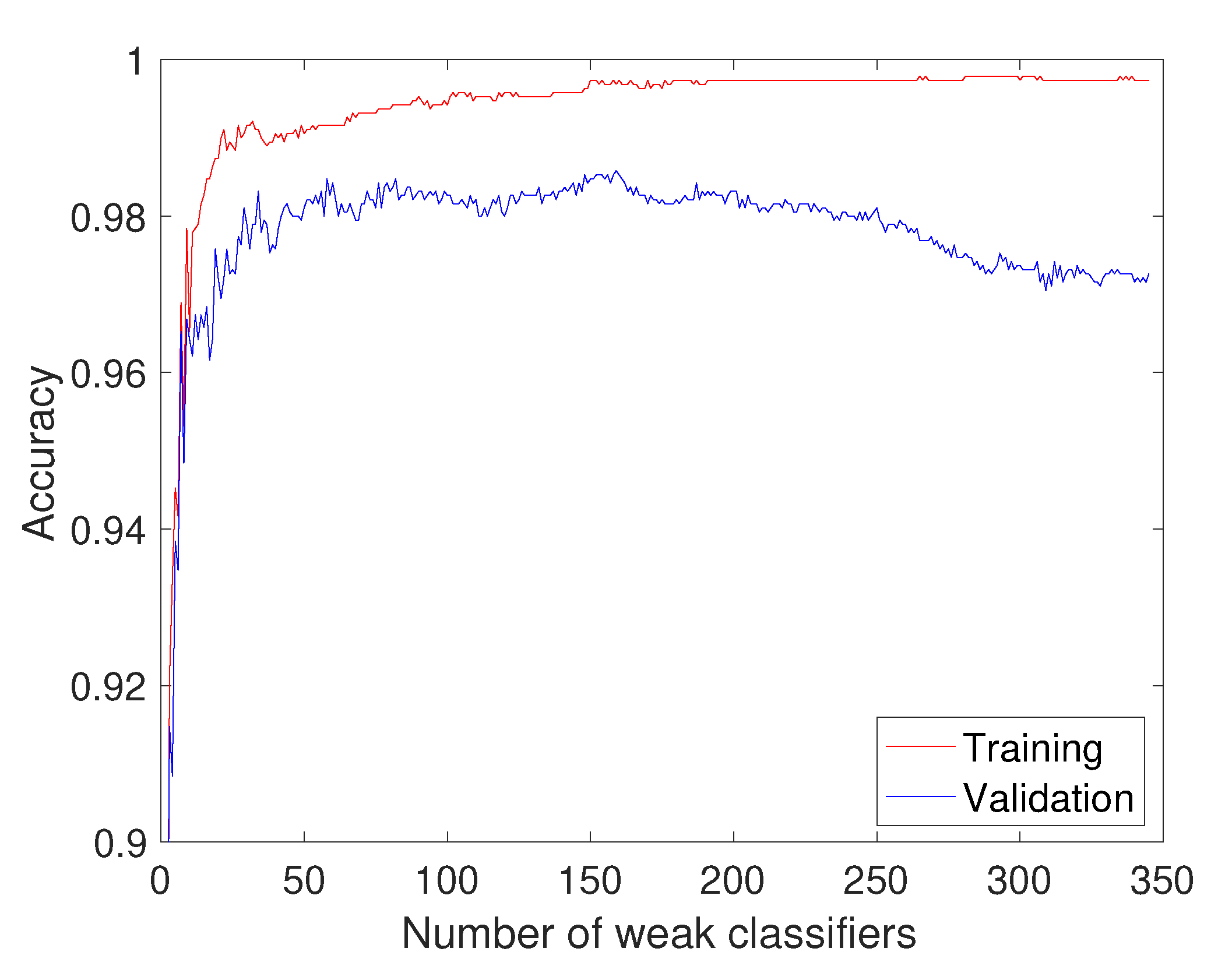Figure 6 illustrates the ROC curves for all three parameters. In addition, we calculate the accuracy of the classifier when the number of weak classifiers is varied. During the variation, we apply the classifier to the validation dataset and to the training dataset and plot the accuracy curves. The results are shown in Figure 7.

As can be derived from Figure 6a, providing a feature pool in which feature descriptors have a minimal size of 10% of the image patch size for the classifier yields best classification results. The classification quality decreases with increasing minimal feature size. This shows that the classification is not impaired but even improved by rather small feature descriptors. Noise and the worker’s positioning seem to have only little effect, if any.

The effect of different amounts of training samples are shown in Figure 6b. As can be seen, the classification quality increases up to a total number of 1600 training samples. From then on, the quality starts to decrease again. This shows that the classifier looses essential features that describe a construction worker in general terms if more than 800 positive and negative samples are used.

As Figure 6a depicts, the general classification quality increases with the number of the cascaded weak classifiers. Nevertheless, the ROC curves of classifiers consisting of more than 100 weak classifiers resemble each other closely for very small FPRs. Since a classifier’s FPR is inversely proportional to its precision, we focus our further evaluation on those small FPRs to ensure a preferably high precision which is mandatory for a proper functioning of our monitoring approach. Although the general performance of the largest cascade exceeds that of all others, the classifier consisting of 152 weak classifiers yields the lowest FPR up to a TPR of 96.2%.

The findings in Figure 6c are also supported by the results in Figure 7. The evaluation up to 150 weak classifiers shows that, in general, the accuracy of the classifier increases. If the classifier contains 152 weak classifiers, it reaches an accuracy of 98% on the validation set. Above 150 weak classifiers, the accuracy of the classifier decreases slightly on the validation set. In contrast, the accuracy increases slightly on the training set. This gives rise to suggesting a slight overfitting.

Based on these findings, we conclusively train a soft cascaded classifier for the application in our approach to the monitoring of workers on construction sites. We provide a pool of feature descriptors consisting of Haar-like features and five-bin color histograms. We add feature descriptors beginning with a size corresponding to 10% of the samples’ sizes and iteratively increase their sizes by further 10% up to a size of 100% of the samples’ sizes. For training, we initially provide 800 samples, each positive and negative, randomly chosen from our training dataset. We then let AdaBoost choose 152 weak classifiers during training which classify the set of training samples best. This halves the time required for the later classification process while retaining an acceptable detection rate. After calibrating this soft cascaded classifier and integrating it into our classical detection setup, we are able to process images at about 28 fps, which even exceeds the frame rate of the camera used for our experiments.

3.2. Optimization of YOLOv3

Prior experiments showed that YOLO’s detection results are considerably robust concerning changes in hyperparameters such as the learning rate, momentum or weight decay. According to these experiments, an optimization of these parameters would not significantly improve the detection results. Therefore, we use these already empirically collected values in our work and do not perform any fine tuning. The most important factor, however, is the size of the input image, since this influences both the detection speed and the precision of the detector. Thus, we conduct a grid search to find the optimal input image size for our purpose. For this purpose, we measure the detection speed in milliseconds (ms) for each image size and calculate the mean Average Precision (mAP) to determine the detection accuracy. Due to YOLO’s downsampling architecture the input image size should be a multiple of 32 px in width and height. We begin the grid search at a factor of 13 for both image dimensions resulting in an image size of 416 × 416 px and gradually increase the factor by 3 up to a final input image size of 800 × 800 px. All these instances of YOLO are trained on the entire training dataset described in Section 2.1 and are evaluated on the validation dataset.

We found that the detection accuracy generally rises with an increasing image size, although the detection speed drops simultaneously (see

Table 1. The results of detection accuracy and detection speed for different image sizes.

Image Size (px)	Detection Speed (ms)	mAP
416 × 416	46	72.9
512 × 512	56	75.2
608 × 608	67	78.5
704 × 704	83	80.3
800 × 800	97	82.7

). At the maximum image size of 800 × 800 px, YOLO yields the best detection accuracy. The processing time for a single image, however, is 97 ms which corresponds to about 10 fps when processing each image of a video. With a processing time of 46 ms per image (22 fps), using the minimal input image size is still too slow to run the detection on every single frame of our video sequences in real-time. Since our camera captures frames at 25 fps, we decided to use an input image size of 608 × 608 px as tradeoff. This way, we are able to process at least every second frame with a desirable precision.

4. Results

In our experiments, we examined the detection quality as well as the capabilities of the approaches, as the basis of a tracking system. To determine their detection quality, we applied both optimized approaches to our test data (see Section 4.1). Afterwards, we used both detection methods for tracker initialization and the recognition of already tracked workers. We examined the precision of the resulting tracks as well as the general ability to accurately identify construction workers, as shown in Section 4.2.

4.1. Detection Quality

To contrast the performances of the optimized detection methods introduced in this paper, we applied both methods to the evaluation dataset described in Section 2.1. For the comparison, we adduced the particular precision and recall of each method on this dataset. Since tracking the workers in a centimeter-perfect manner is usually not required, we defined an Intersection over Union (IoU) value of at least 0.6 to be sufficient to indicate a true positive detection. On our evaluation data, the classical approach exhibits a recall of 96.2% with 99.8% precision. Contrarily, YOLO only achieves a recall of 88.2% with a similar precision of 99.2% using a confidence threshold of 0.9. Even reducing the threshold to 0.5 results in a recall of only 93.5% while precision drops to 97.0%.

4.2. Tracking

Keeping track of the workers is the main purpose of monitoring applications. Accordingly, the tracking should be preferably accurate to provide satisfying results. The detectors of such monitoring systems are the key components for a reliable tracking as their detections serve as initializations and updates for the tracks. In this experiment, we compared the performances of both detectors developed in this paper with respect to the aforementioned requirements. We applied Kalman filtering to their detections to implement a simple and easy to evaluate tracking system.

Each generated tracker has the same dimension during evaluation. The selected size was set manually before, so that the rectangle completely encloses the construction worker in the center of the image. If the detector does not detect a construction worker who is already tracked, the Kalman filter determines its next position only using the prediction. This allows tracking a construction worker who is in motion but is covered, for example, by an object temporarily. Since the accuracy of the position determination decreases without correction of the motion model, these predictions are executed up to a maximum of one second. Otherwise, the track is erased and a new one is set up for the construction worker when the detector detects him again. The prediction is also used to mark the direction of the worker’s movement in the image. For this, the next position in the current image is predicted. Construction workers who move towards a dangerous area can be better identified this way.

The precision and continuity of the underlying detector primarily determines the accuracy and robustness of the tracks. We relied on the approach of Xiao and Zhu [36] to measure these metrics. They proposed the average sequence overlap score (AOS) and center location error ratio (CER) measures for accuracy and track length (TL) for robustness. Ambiguity errors caused by tracks crossing each other are not taken into account since this is a feature of the tracker rather than of the detector. We adapt those metrics to fit to our experimental setup, as shown in Equations (2)–(4).

$$\begin{array}{cc}\hfill \mathrm{AOS}& =\frac{1}{n}\sum _{t=1}^n\frac{A_t^G\cap A_t^T}{A_t^G\cup A_t^T},\hfill \end{array}$$

(2)

$$\begin{array}{cc}\hfill \mathrm{CER}& =\frac{1}{n}\sum _{t=1}^n\frac{\left|\right|C_t^G-C_t^T{\left|\right|}_2}{\mathrm{size}\left(A_t^G\right)},\hfill \end{array}$$

(3)

$$\begin{array}{cc}\hfill \mathrm{TL}& =\frac{n}{N},\hfill \end{array}$$

(4)

where t represents the current time step, n denotes the number of video frames in which a worker is tracked and N is the number of frames in which the worker is present. The worker’s bounding box areas are indicated by A and their centers by C where the superscripts G and T mark ground truth and tracked bounding boxes, respectively. Finally, $\left|\right|\circ {\left|\right|}_2$ denotes the two dimensional euclidean distance and $\mathrm{size}(\circ )$ represents the two dimensional size of an area.

For an eligible comparison of their performances, we evaluated the tracking systems, emerging from each detector combined with Kalman filtering, to identical scenes of construction sites. These scenes are chosen as described in Section 2.1. None of them have been shown to any detector before, neither during training nor during calibration and validation. In the following, we refer to Scene 1 as the scene of four pedestrian workers from the video sequence which is well illuminated, while Scene 2 denotes its overexposed counterpart from the other sequence. The scene showing a car approaching a worker is referred to as Scene 3. The tracking results using the classical detection approach are given in Section 4.2.1. Section 4.2.2 discusses the results of the tracker relying on YOLOv3.

4.2.1. Tracking Results Using a Classical Machine Learning Detector

We applied the tracking system based on the classical machine learning detector to all three evaluation scenes. To each resulting track, a random ID was assigned. Further, we determined the AOS, CER and TL for each track separately. The performance of this system on each of the three evaluation scenes is summarized in

Table 2. Results of the classical machine learning tracking system applied to all three evaluation scenes. For each scene the resulting measures according to Equations (2)–(4) are given. Tracking IDs are assigned randomly to each particular track. The last row highlights the performance of this system averaged over all scenes.

	ID	AOS	CER	TL
Scene 1	0	0.92	0.002	0.97
	5	0.65	0.004	0.92
	8	0.90	0.002	0.99
	9	0.87	0.002	1
Scene 2	1	0.69	0.004	0.92
	2	0.88	0.002	0.95
	3	0.79	0.003	0.97
	4	0.88	0.002	0.88
Scene 3	0	0.82	0.004	1
Average		0.82	0.003	0.96

.

The results indicate a significant decrease in tracking quality for overexposed scenes. This becomes clear when comparing the results of Track 5 with those of the other tracks of the first scene. As shown in Figure 8, Track 5 is located in a highly overexposed section of the scene, whereas the other tracks traverse well-illuminated sections only. This complicates the detection and the tracking consequently results in an inaccurate location, as illustrated in Figure 8a. This figure shows the AOS measure by comparing ground truth data in green to the actual tracks in red and the CER measure by blue lines indicating the distance between the labels’ centers. As can be seen, Tracks 0 and 8 in the well-illuminated area match the ground truth closely and their centers are also close to each other. In contrast, the overlapping area of Track 5 in the highly overexposed section and its corresponding ground truth label is substantially smaller, whereas their centers’ distance is considerably large. Such deviations during the tracking impair its accuracy which becomes visible from the jagged walking path determined for Track 5 in Figure 8b. This is also supported by the TL of only 0.92. Workers in overexposed areas are harder to detect so that the tracking begins delayed, which results in a shortened track length.

In Scene 2, these effects are much less pronounced since the scene is only slightly overexposed. As the comparison of the AOS shows, the difference in the labels’ overlap of Scenes 1 and 2 is only $0.025$ on average, and, even if the outlier (Track 5) in Scene 1 is disregarded, the difference raises to only about $0.086$. The average TL in this scene also decreases only moderately compared to Scene 1. By depicting an example of Scene 2, Figure 9a illustrates that the quality of our tracking approach is sufficient even on slightly overexposed scenes. This finding is supported by measuring the TL and the CER. Both do not vary significantly from Scene 1 to Scene 2. All construction workers are consistently tracked almost throughout the entire duration of both scenes. By applying the tracking system to Scene 3, we show its behavior in the case of moving objects which are not pedestrian construction workers. The results for Scene 3 in Table 2 depict that only one track is set up. As graphically confirmed by Figure 9b, this track belongs to the only worker in this scene. The worker is tracked successfully and no further tracks for the non-worker objects are mistakenly generated. Again, the AOS achieved by the classical system is within an acceptable range, and CER and TL confirm that the worker is tracked consistently throughout the whole scene’s duration.

4.2.2. Tracking Results Using a Deep Learning Detector

To ensure a proper comparison, the evaluation of the deep learning-based tracking system is done analogously to the evaluation of the classical approach. Again, IDs are assigned randomly to the tracks, and the accuracy and robustness metrics are determined per track.

Table 3. Results of the deep learning-based tracking system applied to all three evaluation scenes. For each scene, the resulting measures according to Equations (2)–(4) are given. Tracking IDs are assigned randomly to each particular track. The last row highlights the performance of this system averaged over all scenes.

	ID	AOS	CER	TL
Scene 1	0	0.94	0.002	0.98
	1	0.87	0.003	0.98
	2	0.96	0.002	1
	5	0.98	0.002	0.95
Scene 2	0	0.96	0.001	0.99
	1	0.95	0.005	1
	2	0.98	0.002	0.99
	3	0.90	0.004	1
Scene 3	0	0.98	0.002	0.98
Average		0.95	0.003	0.98

summarizes the performance results of the tracking.

The tracking system exhibits a satisfactory performance on average over all sequences. Especially on well-illuminated scenes, a high accuracy is provided as indicated by the AOS and CER of Scene 1. The system’s performance on this scene is very robust since all workers were tracked almost over the entire length of this video sequence. However, Track 1, which is located in a heavily overexposed area, shows that overexposure affects the quality of the tracking. As the TL shows, the track remains robust, but the accuracy measured by the AOS decreases by about 10% This is also confirmed by a slight increase in the CER. Nevertheless, the system performs very well if the scene is only slightly overexposed as is the case in Scene 2. Here, the AOS barely indicates any negative effects despite the overexposure. Only the CER shows a minor increase. Similar to the highly overexposed case, the TL measurements again emphasize the tracking system’s robustness, although slight overexposure is present on the entire scene.

Besides this, the results of this experiment also show that the system does not confuse construction workers with any other object in the scenes. As Table 3 shows, the correct number of tracks was set for each scene. Alongside the four construction workers, Scenes 1 and 2 include static construction related objects, such as traffic cones and barriers. These stay correctly undetected and untracked during the course of the video sequences. Moving objects such as the car in Scene 3 also remain correctly unnoticed by the tracker.

5. Discussion

As shown by our experiment regarding the detection quality, both methods outperform the approach of Luo et al. [24] by far. While Luo et al. achieved a precision of 75.1%, our approaches reach 99.8% and 99.2%, respectively. A proper comparison of the results is delicate since the datasets used for training and evaluation differ from each other. However, tests using YOLO with the same input image size as proposed by Luo et al. yield similar results, which indicates at least a weak comparability of the setups. This confirms that the input image size is a crucial parameter for a proper detection when using YOLO, as the objects to be detected shrink proportionally to the size of the images. Nevertheless, this experiment also shows that the results of the classical method exceed those of YOLO by about 5%. As mentioned above, the image size may be a reason for this. The classical approach operates on the original high resolution, exhibiting more detailed features than the drastically downscaled images used by YOLO. A second reason may arise from the limited dataset since it is known that CNNs require a vast amount of training data. The number of provided training samples may have been too small to sufficiently adapt to the class of workers, although we deliberately used a pre-trained network which already developed general feature descriptors for classification. On the contrary, the findings in Section 3.1 highlight that classical computer vision approaches cope significantly better with fewer samples than CNNs.

Both reasons emphasize common practical issues concerning data gathered in the context of construction site monitoring. Since computer vision approaches are rarely applied in the field, dataset generation has rarely been regarded a subject until now. Beyond this, generating a reasonable dataset covering all environmental and lighting conditions is extremely time-consuming and tedious. Given such a dataset, the small size of the pedestrian workers within the images remains to be a limiting factor. Thus, choosing a classical detection approach over a CNN is desirable to obtain the best detection results for the purpose of monitoring pedestrian workers.

However, our tracking experiments showed that both approaches yield suitable results. As can be seen from the results of Scene 1, the evaluated systems perform similarly well on a well-illuminated environment. Both approaches exhibit an excellent accuracy with very low CER and high AOS of about 90%. Furthermore, the high TL rates indicate their robustness. The slight deviations from the optimum are mainly due to workers entering and leaving the scene. In these situations, workers are located at the image boarders and may be only partly visible. This complicates the detection of the workers so that tracks may be set up late or may terminate early. Apart from these effects, the tracking performed by both approaches is very precise despite the CNN’s limitations in detection quality and speed. This shows that even simple tracking methods can compensate for lower detection rates. However, Scene 1 also shows that both approaches have issues with high overexposure. In both cases, the AOS of the regarding track drops noticeably accompanied by a raise in CER. The worker is still tracked sufficiently by both systems but the accuracy dramatically suffers from the overexposure. The CNN-based approach seems to cope with this issue slightly better than the classical system. This is no reliable statement yet as there is only a single instance of evidence available in the data. The results of Scene 2 provide further insights into the subject of overexposure. On this scene, the TL rates remain almost stable indicating a satisfying robustness. This ensures reliable tracking with both tracking systems despite a certain degree of overexposure. However, the CNN-based approach achieves significantly better AOS rates in this slightly overexposed environment. The CER rates fluctuate more than with the classical approach. On the one hand, the considerable decrease in AOS shows that the classical system has difficulties in identifying the worker’s dimensions precisely when overexposed. This is also supported by the findings regarding the overexposed Track 5 of Scene 1. At the same time, the stable CER rates indicate that the worker’s centers—and thereby their locations—are recognized with high accuracy. On the other hand, the CNN-based system reveals its weakness concerning a precise localization, as shown by the varying CER. Instead, it accurately determines a worker’s dimensions despite aggravated conditions. With this knowledge, the size of the detected area could in the future be passed to the tracker so that the worker is for the most part completely marked on the image. For the classical approach, a fixed size of the tracking box would be more suitable, which has to be determined in advance depending on the camera height.

This points out that both approaches possess certain pros and cons. Under ideal conditions both perform similarly well but as conditions change, they start focusing on different aspects. While the classical approach precisely keeps track of the worker’s locations, the CNN-based system accurately recognizes their dimensions. Accordingly, a conclusive decision has to be made with respect to the demands of particular applications.

6. Conclusions

In this study, we investigated whether deep learning methods surpass classical approaches on construction worker monitoring despite their limitations. We chose YOLOv3 for the CNN and a classical approach based on a soft cascaded classifier as representatives for our comparison. The trained detectors were then embedded in a tracking system to track construction workers in video sequences. To evaluate the tracking systems under various conditions, we generated different video sequences. These contain different environmental and lighting conditions as well as stationary and moving non-worker objects. Both tracking systems were applied to the same sequences to ensure a proper comparison.

As our experiments showed, the classical approach clearly outperforms the CNN on the detection task in terms of quality and speed. The lack of quality is most likely due to an insufficient amount of training data and the heavy downscaling of the images. The low detection speed of substantially less than 22 fps is affiliated to the high computational costs. However, the tracking experiment showed that the CNN’s drawbacks are fully compensated even by a simple tracking method. Both approaches showed satisfying results when tracking workers under ideal conditions. They were even able to suppress a false tracking of any stationary or moving non-worker object. Nevertheless, both tracking systems reveal deficiencies when applied to overexposed conditions. While the CNN keeps precise track of the worker’s dimensions, localization becomes inaccurate. The classical approach behaves exactly vice versa. According to these findings, there is no optimal monitoring approach in general. A suitable approach has to be chosen with respect to the demands of the particular application.

With our example scenarios, we showed that with both approaches a satisfactory tracking of the construction workers from the top view is possible. Nevertheless, it would be an advantage to know whether satisfactory tracking is also achieved with more complex work processes with different moving machines, different construction site constellations and different weather conditions. Therefore, future work should compare the presented tracking approaches with scenes that have a different focus. In this case, optical flow techniques can additionally be used to enable tracking also with cameras mounted, e.g., on the crane boom. The background subtraction would consider known crane movements and thus dynamically changing backgrounds would be taken into account. Furthermore, future work should concentrate on substantially increasing the size of the datasets. By this, the training of CNN-based approaches can be improved. This helps the detector to develop a better generalization ability, which may advance the tracking results especially under difficult conditions. Reasonable strategies for the extension may be alternative data augmentation techniques as well as computer generated data.