Chemical Composition and Source Apportionment of PM₁₀ in a Green-Roof Primary School Building

Featured Application

Introductory Article of the MDPI Special Issue “New Challenges for Indoor Air Quality”.

Abstract

Research on air quality issues in recently refurbished educational buildings is relatively limited. However, it is an important topic as students are often exposed to high concentrations of air pollutants, especially in urban environments. This study presents the results of a 25-day experimental campaign that took place in a primary school located in a densely built-up area, which retains a green roof system (GRS). All measurements refer to mass concentrations and chemical analysis of PM₁₀ (particulate matter less than 10 micrometers), and they were implemented simultaneously on the GRS and within the classroom (C3) below during different periods of the year. The results demonstrated relatively low levels of PM₁₀ in both experimental points, with the highest mean value of 72.02 μg m⁻³ observed outdoors during the cold period. Elemental carbon (EC) was also found be higher in the ambient environment (with a mean value of 2.78 μg m⁻³), while organic carbon (OC) was relatively balanced between the two monitoring sites. Moreover, sulfate was found to be the most abundant water soluble anion (2.57 μg m⁻³), mainly originating from ambient primary SO₂ and penetrating into the classroom from windows. Additionally, the crustal origin of particles was shown in trace metals, where Al and Fe prevailed (9.55% and 8.68%, respectively, of the total PM₁₀). Nevertheless, infiltration of outdoor particles within the classroom was found to affect indoor sources of metals. Finally, source apportionment using a positive matrix factorization (PMF) receptor model demonstrated six main factors of emissions, the most important of which were vehicles and biomass burning (30.30% contribution), along with resuspension of PM₁₀ within the classroom from human activities (29.89% contribution). Seasonal variations seem to play a key role in the results.

1. Introduction

In most European countries, pupils spend up to 80% of their day indoors and most of the time in school classrooms, compared to other places, excluding their homes [1]. Therefore indoor air quality (IAQ) in classrooms is an important issue of scientific interest as children inhale more air than adults, because of their low weight, and because of the limited immune system development in children [2,3,4,5]. Numerous researchers have attempted to associate environmental conditions within the classrooms with various respiratory symptoms of students [6,7,8,9]. In addition, other type of issues, such as thermal discomfort and decrease of productivity during lessons, were reported by Lee and Chang [10].

In Europe, Madureira et al. [11] performed measurements in 73 classrooms from 27 elementary schools in Portugal and found high concentrations of PM_2.5, PM₁₀ and airborne fungi. In addition, different IAQ levels were correlated with health symptoms by using scientific questionnaires. Within that frame, the study of Rufo et al. [12] reported a 40% decrease in airborne particles because of more frequent cleaning and ventilation. Within three elementary schools of central Italy, Stabile et al. [13] investigated the influence of seasonality on their measurements, concluding that during warm months there was a strong influence of ambient particles to indoor concentrations due to emissions from vehicles. In Poland, measurements of Mainka et al. [14] at two nursery schools during winter presented increased levels of PM₁₀, indicating internal sources of emissions. A study by Canha et al. [15], in 51 classrooms from 17 schools of central France, showed that 91% of classrooms demonstrated inadequate ventilation levels, while student activities affected the levels of IAQ. Similar experiments have also been carried out in classrooms of many other European countries [16,17,18,19,20,21,22,23].

Furthermore, in Asia, Goyal et al. [24] investigated the IAQ conditions of a primary school in India, near a busy street. The researchers concluded that high levels of outdoor PM₁₀ influenced the respective concentrations indoors, while meteorological parameters also played a key role in the results. Additionally, the research of Yang et al. [25] in 55 refurbished schools of South Korea showed high levels of formaldehyde (HCHO), mainly due to the massive use of MDF type of wood. The experimental campaign of Ismail et al. [26] in three primary schools in Malaysia highlighted the differences between particle concentrations depending on sampling location (urban, suburb or outskirts). More recently, the research of Ma et al. [27] in classrooms of Northeast China, a region with significant low average annual temperatures, showed that closed windows along with high occupancy levels can lead to poor IAQ levels. The importance of extreme meteorological conditions was also highlighted by Abdel-Salam et al. [28] for 16 Qatari schools. This research reports increased levels of internal PM₁₀ due to external dust transfer episodes.

In USA, Petronella et al. [29] found relatively low PM₁₀ concentrations at a school in Texas, but with elevated concentrations of airborne fungi. Similar results were also found in the study of Leventin et al. [30] within 14 schools in different cities in the US. Moreover, in 64 Michigan schools, Godwin et al. [31] recorded high CO₂ concentrations and inadequate natural ventilation rates, while Shendel et al. [32] reported that these two parameters were the main reasons for the selective absence of pupils from Washington and Idaho classrooms. However, levels of particulate matter were measured below their respective limits. More recent research by Majd et al. [33] in 16 Baltimore schools highlighted the issue of the influx of external air pollutants into the interior of buildings through natural ventilation.

Studies from the rest of the world, such as Guo et al. [34] at a primary school in Australia, emphasized the influence of garden maintenance work on internal concentrations of PM_2.5. In addition, in Brazil, Avigo et al. [35] reported that a high proportion of soot was found in the measured suspended particles of two school buildings. Additionally, the research of Mustapha et al. [36] in classrooms of the Niger Delta highlighted the impact of ambient air pollution on IAQ.

In Greece, Diapouli et al. [37] reported that internal concentrations of airborne particles in seven primary schools in Athens were strongly influenced by resuspension due to the activities of pupils. This research, along with the respective work of Chaloulakou et al. [38], Siskos et al. [39] and Synnefa et al. [40] comprised some of the first research efforts concerning IAQ within Greek schools. More recently, Dorizas et al. [41] implemented IAQ measurements in nine naturally ventilated schools in various areas of Athens. They concluded that the levels of indoor PM₁₀ were extremely high and mainly originated from chalk. Additionally, by using scientific questionnaires, students associated low levels of IAQ with elevated temperature values, highlighting the importance of seasonality. Relevant publications such as Dimoudi et al. [42], Dascalaki et al. [43] and Kalimeri et al. [44] reported similar results about IAQ and energy savings in Greek classrooms.

Referring to school buildings with a green roof system (GRS), Kim et al. [45] and Hong et al. [46] reported satisfactory indoor temperature levels and reduced CO₂ emissions in South Korean classrooms compared to conventional buildings. In Mediterranean climates, Perini et al. [47] noted that the addition of a GRS improved thermal comfort conditions of an educational institution in Italy. Nevertheless, the vegetation type also plays an important role in both energy savings (low water requirements) and reduction of gaseous pollutants, according to Ascione et al. [48]. Additionally, it should be noted that green roofs can lead to a reduction of ambient PM₁₀ (and other air pollutants) only if they are installed on several buildings in the same location. In particular, Yang et al. [49] highlighted a PM₁₀ reduction of 14% after the installation of 170 green roofs in Chicago, USA, while a 10–20% GRS extension on buildings in Toronto led to significant improvement of air quality, as Currie and Bass [50] noted. More recently, the study of Speak et al. [51] highlighted that some specific kinds of grass on roofs in Manchester could effectively remove airborne particulate matters.

From all the above, it becomes obvious that from the large number of studies in different climatic zones, IAQ depends on occupancy, ventilation patterns, location and outdoor sources. However, few IAQ studies at schools to which an intervention for energy upgrade has been applied, such as the installation of a GRS, exist. To this direction, the present study aims to investigate the concentration levels, chemical composition and potential sources contributing to coarse particulate matter (PM₁₀) in the indoor and outdoor environments of a primary school, which retains a GRS. As source apportionment studies inside classrooms are limited, this work will add information on the investigation of PM sources in the school microenvironment and, consequently, on the exposure of the child population.

2. Materials and Methods

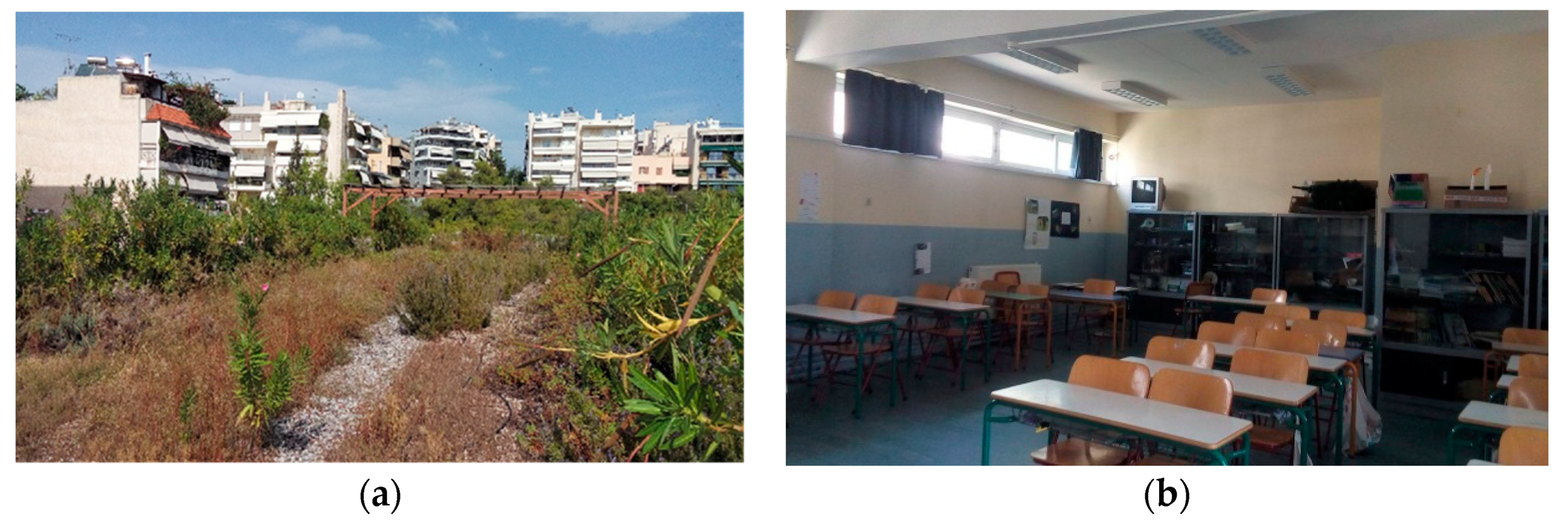
2.1. Sampling Periods and Location

For the scope of the study, a primary school partly retaining a GRS was selected in order to investigate the IAQ and particulate sources of emissions. PM₁₀ mass and chemical composition measurements were conducted in and out of the building. After obtaining the results, a positive matrix factorization model was applied to estimate the sources.

Measurements were performed during 25 selected days from January to June 2017 and were obtained simultaneously from the GRS and the classrooms beneath it (C3). The experimental campaign was separated into cold (19th of January to 29th of March) and warm (3rd of April to 19th of June) periods. During the cold period, the classroom was heated via the central heating system of the building (oil boiler with radiators).

The second primary school is located in Nea Smyrni, a southern suburb in the city of Athens, Greece and close to the port of Piraeus. It is a densely built, highly trafficked, mostly residential area. Outdoor concentrations of air pollutants are mainly derived from port activities (south), vehicles and central heating. The school retains two floors and is located close to a road with high traffic. The building was constructed in 1954 and refurbished in 2000, while the GRS was added in 2008.

The GRS covers an area of 374 m². The type of the GRS is extensive, lightweight (less than 150 kg/m²) and with light soil of 150 mm thickness and low vegetation. The plants do not require large amounts of water, which is provided by an automatic watering system.

Classroom C3 is naturally ventilated by window openings. Window frames have a glazing area of approximately 2.5–3 m² and are situated close to the ceiling due to safety reasons. During the cold period they remained open for a short time before and after the lectures. However, amid the warm period (April to June), the windows remained open during class hours as well. Cleaning service was operating daily after the end of lectures. The room volume is about 210 m³, and the number of pupils that year was 24. During the lessons, a logbook of activities was kept to annotate human activities and various school events. Lessons took place from 8:30 to 13:30 daily. Figure 1a,b depicts the two experimental areas.

2.2. Experimental Equipment

In situ measurements were implemented indoors and outdoors with the use of portable equipment. More specifically, within classroom C3, a SKC sampler was installed, operating at 4 L/min and equipped with a size-selective inlet for PM₁₀. Air pollutants were collected on quartz filters of 37 mm diameter. On the GRS, a low volume controlled flow ratio (2.3 m³/h) sampler (Derenda LVS 3.1/PNS 3.1–15) was used for outdoor sampling, based on the European standard method EN 12341:2014 [52]. Particles were collected on 47 mm preconditioned quartz filters, which were protected in plastic holders before and after sampling. Each filter corresponds to a daily measurement. Particle mass concentration was conducted gravimetrically using an electronic microbalance (Mettler Toledo MX-5), with a resolution of 10⁻⁶ g, within a weighing room under controlled climatic conditions (temperature 20 ± 1 °C and relative humidity 50 ± 5%). Moreover, the instrumentation also included ambient temperature and relative humidity sensors (Tinytag Plus 2 thermo-hygrometers with a range from −25 to 85 °C for temperature and from 0 to 100% for relative humidity and accuracy of ±0.6 °C and ±3.0%, respectively). It should be noted that daily values of wind speed and direction were obtained by a local meteorological station (37°57′00″N, 23°43′00″E).

For organic/elemental carbon (OC/EC) analysis, a thermo–optical ECOC Sunset Laboratory analyzer was used. In the analyzer, samples were thermally desorbed from the filter medium under an inert helium atmosphere followed by an oxidizing atmosphere using carefully controlled heating lamps. A flame ionization detector (FID) was used to monitor the analysis. More specifically, the method for measuring OC and EC in ambient particulate matter samples deposited on filters was based on the volatilization and oxidation of carbon-containing PM components. After the quantification of the carbonaceous gases released, an optical correction for the charring of OC to EC in the process (the thermal-optical method) occurred. The described procedure is a thermal-optical transmittance/reflectance (TOT/TOR) method [53]. For the analysis, tissue quartz filters were used, while the EUSAAR2 protocol was followed. The instrument’s limit of detection (LOD) was 0.2 µgC cm⁻², and the analytical uncertainty was equal to ± (concentration × 0.05) + instrument blank concentration.

Water-soluble anions (Cl⁻, NO₃⁻, NO₂⁻, Br⁻, PO₄³⁻ and SO₄²⁻) were investigated using suppressed ion chromatography (IC). In particular, a DIONEX DC ICS-5000 system was used for the evaluation of ion concentrations, since it offers a full range of Reagent-Free™ IC (RFIC™) components. RFIC-EG combines automated eluent generation and self-regenerating suppression. Regarding the chemical process elaborated, a tissue quartz filter was used for ultrasonic extraction, using 6 mL of Milli-Q water and 0.5 mL isopropanol. Then, the solution was injected to the ionic chromatographer. The LOD ranged between 0.01 and 0.11 µg mL⁻¹. Uncertainty (95%, k = 2) ranged between 5.61% and 9.31%, respectively.

PM sample analysis of metals (Al, As, Ba, Cd, Co, Cr, Cs, Cu, Fe, Mn, Ni, Pb, Sr, Tl, V and Zn) was performed according to the procedure described by Romanazzi et al. [54]. Samples were digested using a mixture of HNO₃ (suprapur 65%) and H₂O₂ (suprapur 30%) in a microwave digestion system (CEM; Matthews NC USA). All digested samples were analyzed through inductively coupled plasma mass spectrometry (ICP-MS) by a Thermo Scientific ICAP Qc (Waltham, MA, USA). Measurements were implemented in a single collision cell mode, with kinetic energy discrimination (KED) using pure He. Matrix induced signal suppressions and instrumental drift were corrected by internal standardization (⁴⁵Sc, ¹⁰³Rh). Analysis of Al, Fe and Cr were implemented by graphite furnace atomic absorption spectrometry (GFAAS) with Zeeman background correction (SpectrAA 640Z; Varian, Mulgrave, Victoria Australia), after digestion of filters with a mixture of HNO₃ (65%), HCl (30%) and HF (40%). Complete solubilization of Cr and aluminosilicates was achieved with this digestion procedure where HF was used. When samples were prepared and analyzed in batches, at least one laboratory blank was evaluated in order to monitor background contamination. Thus, quality control was achieved The LOD was within the range of 0.004–0.20 ng m⁻³ for ICP-MS determined elements and 1.0–2.0 ng m⁻³ for GFAAS determined elements (referring to an air sampled volume of 52 m³).

2.3. Positive Matrix Factorization (PMF)

2.3.1. Model Background

Receptor modeling aims at reconstructing the contribution of emissions from various sources of air pollutants (e.g., particulate matter) based on measurement data (i.e., particles’ chemical compositions) monitored at a specific receptor site. Positive matrix factorization (PMF) is one of the most commonly used receptor models. This model uses a weighting scheme, taking into account errors of the data points, which are used as point-by-point weights. In addition, non-negative constraints are applied so as to obtain physically meaningful factors. The model version available by USEPA (PMF v.5.0) was applied in the present study. The PMF analysis background was described in detail by Paatero [55]. In a few words, the model can be written as

X = GF + E,

(1)

where X is the known n × m matrix of the m measured chemical species in n samples; G is an n × p matrix of the p sources contributions to the samples (time variations); and F is a p × m matrix of source compositions (source profiles). Both G and F are factor matrices to be determined. E is defined as a residual matrix, i.e., the difference between the measurement X and the model Y as a function of factors G and F.

$${{\displaystyle e}}_{ij}={{\displaystyle x}}_{ij}-{{\displaystyle y}}_{ij}={{\displaystyle x}}_{ij}-{\displaystyle \sum _{k=1}^p{{\displaystyle g}}_{ik}}{{\displaystyle f}}_{kj}(i=1,\dots ,n;j=1,\dots ,m;k=1,\dots ,p)$$

(2)

The scope of PMF is to minimize the sum of the squares of the residuals weighted inversely with error estimates of the data points. Furthermore, PMF constrains all of the elements of G and F to be non-negative, meaning that sources cannot have negative species concentrations (f_kj $\ge$ 0) and samples cannot have a negative source contributions (g_ik $\ge$ 0). The task of PMF analysis can thus be described as to minimize Q, which is defined as

$$Q(E)={\displaystyle \sum _{i=1}^n{\displaystyle \sum _{j=1}^m({{\displaystyle e}}_{ij}^{}}}/{{\displaystyle s}}_{ij}{)}^2$$

(3)

where f_kj $\ge$ 0; g_ik $\ge$ 0; and s_ij is the error estimate for x_ij.

Occasionally, other auxiliary equations can be added in order to include information regarding, e.g., chemical profiles for specific sources [56]. These auxiliary equations are applied to the selected solution as constraints, which can lead to a free rotation of the solution with better physical meaning than the original one. Further, a number of rotations blocking zero values can be introduced to the matrix, increasing the rotational stability of the solution.

2.3.2. Input Data Pre-Treatment and Model Runs

The available data from the measurement campaigns were 16 trace elements (Al, As, Ba, Cd, Co, Cr, Cs, Cu, Fe, Mn, Ni, Pb, Sr, Tl, V and Zn), 6 water-soluble anions (Cl⁻, NO₃⁻, NO₂⁻, Br⁻, PO₄³⁻ and SO₄²⁻) and elemental and organic carbon (EC, OC). As, Ba, Co, Cs, Ni, Sr, Tl, V, Zn, NO₂⁻, Br⁻ and PO₄³⁻ were set as “bad” species and excluded from the analysis either due to the high percentage of missing values or their very low signal/noise ratios (<0.2). NO₃⁻, Cu and Cr were set as “weak species” due to their low signal/noise ratios (S/N) or/and poorly scaled residuals (d-matrix). PM₁₀ mass concentration was set as the total variable. Concentration data lower than the detection limit were substituted with one-half of the detection limit, while missing data were substituted with the median value for the specific species [57]. Similarly, uncertainty for data below the detection limit was set equal to 5/6 of the detection limit, while uncertainty for missing data was set equal to 4 times the median concentration. The modeling extra uncertainty was adjusted to 14%.

Therefore, an input matrix of 50 samples and 12 chemical species was inserted in the model, while 30 runs were performed for each testing case, for obtaining Q-value stability. All runs converged, and Q values ranged between ±1.2%. The Q-robust value was lower than 1.5 times the Q-true value for each case, signifying that the impact of the outliers on Q value was not considerable. The optimal number of factors was determined by examining the Q values for PMF solutions resulting from a range of the “number of factors” values without excluding the solution’s physical validity. A range of solutions was examined with different numbers of factors (3–10), but six was the maximum number of factors corresponding to meaningful sources. In fact, when the PMF factors number increased from the optimal, a number of factor profiles were split to profiles with no physical meaning, while the rotational instability of the solution increased significantly. Finally, bootstrap and displacement runs were used for estimating the effect of random errors and the rotational ambiguity of a dataset. In our study, two constraints needed to be applied with the limitation of dQ% being kept at the lowest value of 0.5%: (i) Al: pull up maximally in “resuspension” factor, and (ii) SO₄²⁻: pull up maximally in “secondary sulfate” factor. Compared to the initial results, no substantial changes to either the constrained profiles or the constrained contributions were observed, amplifying the accuracy of the selected solution.

2.4. Statistical Analysis

Statistical software packages including IBM^® SPSS PASW Statistics 18 and Microsoft^® Excel 2013 were used in order to analyze the data. It should be noted that in order to investigate statistically significant differences between sets of variables, the non-parametric Kruskal–Wallis-H test (or one way ANOVA) with p < 0.05 was implemented.

So as to highlight possible sources of indoor particles, enrichment factors were calculated for individual elements in terms of the average elemental composition of the upper continental crust. For each one of the examined metals, Al was used as a reference element, assuming minor contributions of Al as a potential pollutant and considering the upper continental crustal composition reported by Rudnick and Gao [58]. The enrichment factor (EF) of an element E is defined according to the following formula:

EF = (E/R)_air/(E/R)_crust

(4)

where E and R represent the concentrations of examined and reference element, respectively. If EF approaches 1, the earth’s crust is the predominant source of the examined element.

3. Results and Discussion

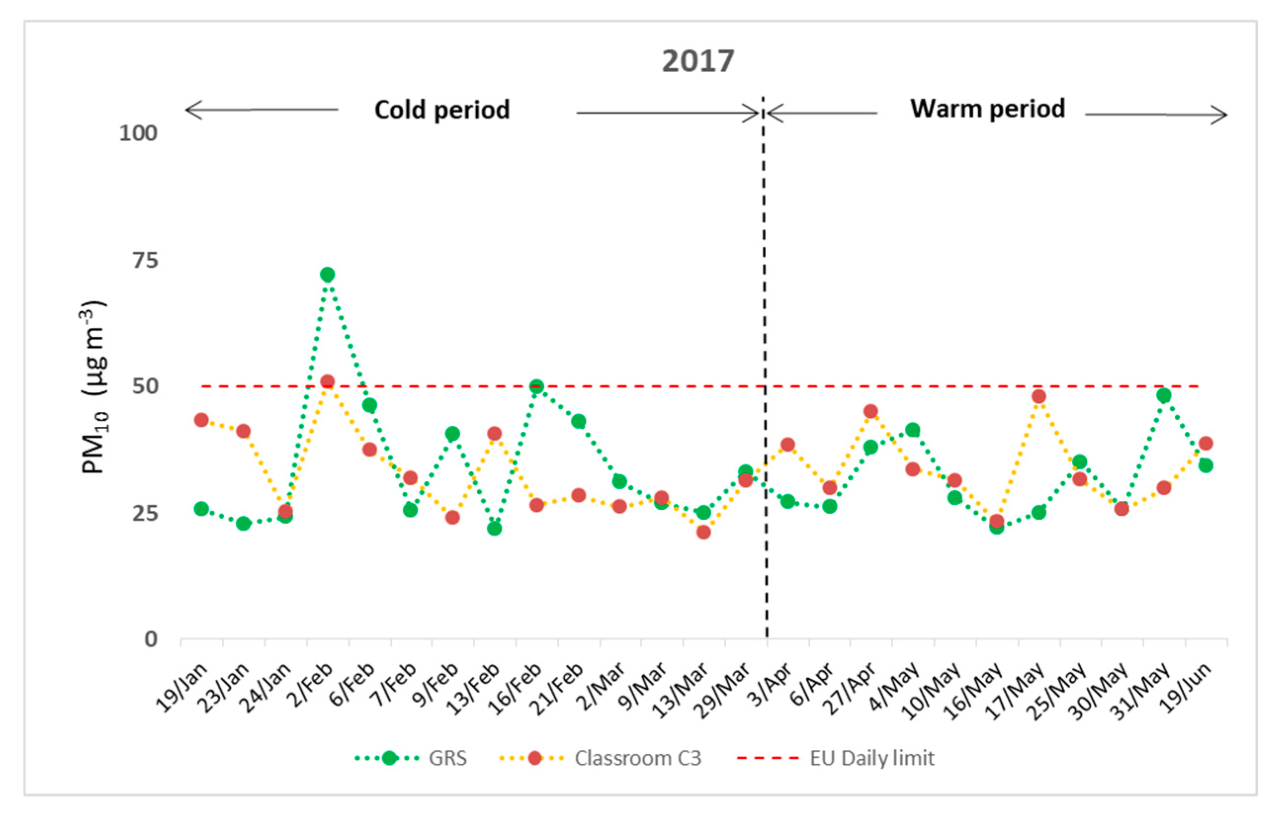
3.1. PM₁₀ Mass Concentration

The mean daily PM₁₀ concentrations recorded on the GRS and within classroom C3 (including class hours), are illustrated, respectively, in Figure 2. However, it should be noted that a limitation of this study was that measurements of ambient PM₁₀ were implemented only on the GRS and the classroom beneath it. No control classroom (with a conventional roof above) was selected. Concentrations of PM₁₀ ranged between 21.88 and 72.02 μg m⁻³ outdoors and from 21.11 to 50.92 μg m⁻³ indoors. It was obvious that PM₁₀, both indoors and outdoors, did not exceed the daily limit of 50 μg m⁻³ proposed by the European Directive 2008/50/EU [59], with the exception of the 2nd of February (cold period). Thus, one may notice that the ambient environment of the school was not severely burdened by coarse airborne particles. Furthermore, seasonal changes seemed to have an important role on the results. During the cold period, 57.14% of ambient measurements were found to be higher on the GRS, mainly because of airborne suspended particles that were emitted as combustion products from fireplaces or other heating systems of the local dwellings. This is also noticed in the publication of Fameli and Assimakopoulos [60]. On the contrary, 63.64% of PM₁₀ recordings amid the warm period were found to be higher in classroom C3. Resuspension of particles due to indoor activities seemed to prevail for most cases. Ambient particulate matter can be directly emitted from vehicles of nearby busy streets or transported by dust transfer episodes, as Fameli and Assimakopoulos [61], Agudelo-Castañeda et al. [62] and Soleimanian et al. [63], report. The significant role of seasonality could also be noticed by the calculation of the indoor to outdoor ratio (I/O) of PM₁₀. For the warm period, the mean I/O value was found to be 1.12, which demonstrates that PM₁₀ concentrations within classroom C3 were slightly higher with respect to GRS. On the other hand, the average I/O ratio for the cold period was 1.04, depicting the elevated levels of external PM₁₀ mainly because of the operation of local heating systems at this time of the year. Additionally, no significant correlation between indoor and outdoor PM₁₀ was found, with Spearman’s rho equal to 0.09 (p = 0.69), probably because of different emission sources and daily window openings. These results are in accordance with the publication of Zwoździak et al. [64], as they reported a higher PM₁₀ I/O ratio during summer than amid winter at a school of Wroclaw.

Regarding the meteorological conditions during the experimental period, the dominant wind direction was of NNW and NW direction (52% of the samples). For 32% of the measurements, the wind blew from the SW direction, while NE and SE directions were also recorded for the rest of the cases. Wind speed remained at relatively low levels for all experimental days with daily average values ranging from 0.5 to 8.7 km/h. Mean daily values of temperature and relative humidity ranged from 6.2 to 23.4 °C and from 48.3 to 94.3%, respectively.

Table 1. Mean daily values of examined meteorological parameters for all experimental days.

Date 2017	Temperature °C	Rel. Humidity %	Wind Speed km/h	Wind Direction Dominant
19/1	10.9	48.9	3.2	NNW
23/1	7.8	74.8	7.2	NNW
24/1	7.8	94.3	4.7	NNW
2/2	9.7	80.5	0.5	NE
6/2	13.8	81.9	3.1	SE
7/2	12.1	66.4	2.4	SE
9/2	10.5	82.9	6.0	NNW
13/2	6.2	69.2	8.4	NNW
16/2	9.5	61.2	6.4	NNW
21/2	12.9	79.2	1.0	SW
2/3	14.8	53.3	5.1	NNW
9/3	11.8	69.7	3.2	NNW
13/3	14.4	61.4	3.2	NW
29/3	14.1	54.8	1.6	SW
3/4	15.8	55.6	1.1	NNW
6/4	17.0	68.7	1.3	SW
27/4	19.2	52.0	1.1	SW
4/5	22.1	56.6	1.6	SW
10/5	22.4	53.2	2.4	SW
16/5	22.2	48.3	8.7	NNW
17/5	18.7	69.8	7.2	NNW
25/5	22.2	71.5	1.3	SW
30/5	22.1	59.5	1.8	NE
31/5	23.4	58.4	1.1	SW
19/6	20.7	71.1	4.7	NNW

summarizes all the investigated meteorological parameters. It should be noted that there was no specific pattern associating wind direction with high or low concentrations of PM₁₀ for the external measurements on the GRS of the building. All data refer to dominant wind directions, as the wind can change several times during the day. The wind speed was found to be negatively correlated with ambient PM₁₀ concentrations, with Spearman’s rho coefficient being −0.56 (p = 0.03). Daily concentrations of ambient PM₁₀ were found elevated (above the respective exposure limit) only on the 2nd of February when the average wind speed was relatively low (0.5 km/h). This demonstrates the dominance of local sources in which strong winds flush airborne particles while calm winds allow the buildup of concentrations, as Karar and Gupta [65] reported. Moreover, on the 24th of January, concentrations of ambient PM₁₀ were found to be decreased mainly because of precipitation (5.4 mm). However, no significant correlations between ambient PM₁₀ and air temperature or relative humidity were depicted, as Spearman’s rho coefficients were found to be 0.16 (p = 0.45) and 0.13 (p = 0.53), respectively, for all samples. This is in accordance with the study of Saraga et al. [66], which suggests that longer time series of data are needed in order to examine the influence of those climatic factors on PM₁₀ concentrations.

Table 2. Spearman correlations of ambient (GRS) PM₁₀, air temperature (T), relative humidity (RH) and wind speed (WS) for all experimental days.

Spearman’s Rho		PM10 (GRS)	T	RH	WS
PM10 (GRS)	Correlation Coefficient	1.00
	Sig. (2-tailed)	-
	N	25.00
T	Correlation Coefficient	0.16	1.00
	Sig. (2-tailed)	0.45	-
	N	25.00	25.00
RH	Correlation Coefficient	0.13	−0.48 *	1.00
	Sig. (2-tailed)	0.53	0.01	-
	N	25.00	25.00	25.00
WS	Correlation Coefficient	−0.56 **	−0.33	0.05	1.00
	Sig. (2-tailed)	0.00	0.11	0.80	-
	N	25.00	25.00	25.00	25.00

** Correlation is significant at the 0.01 level (2-tailed); * correlation is significant at the 0.05 level (2-tailed).

demonstrates the results of all correlation coefficients.

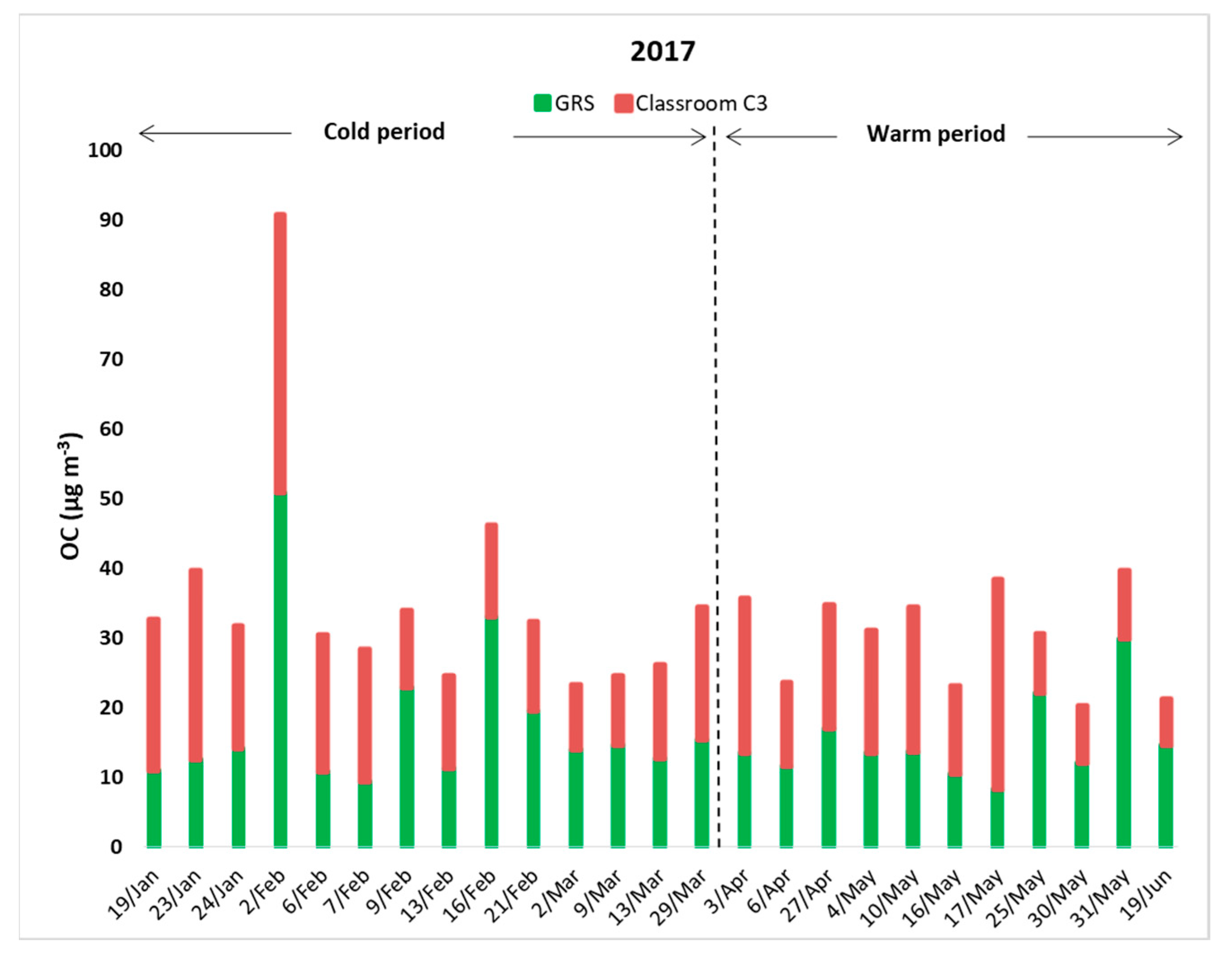
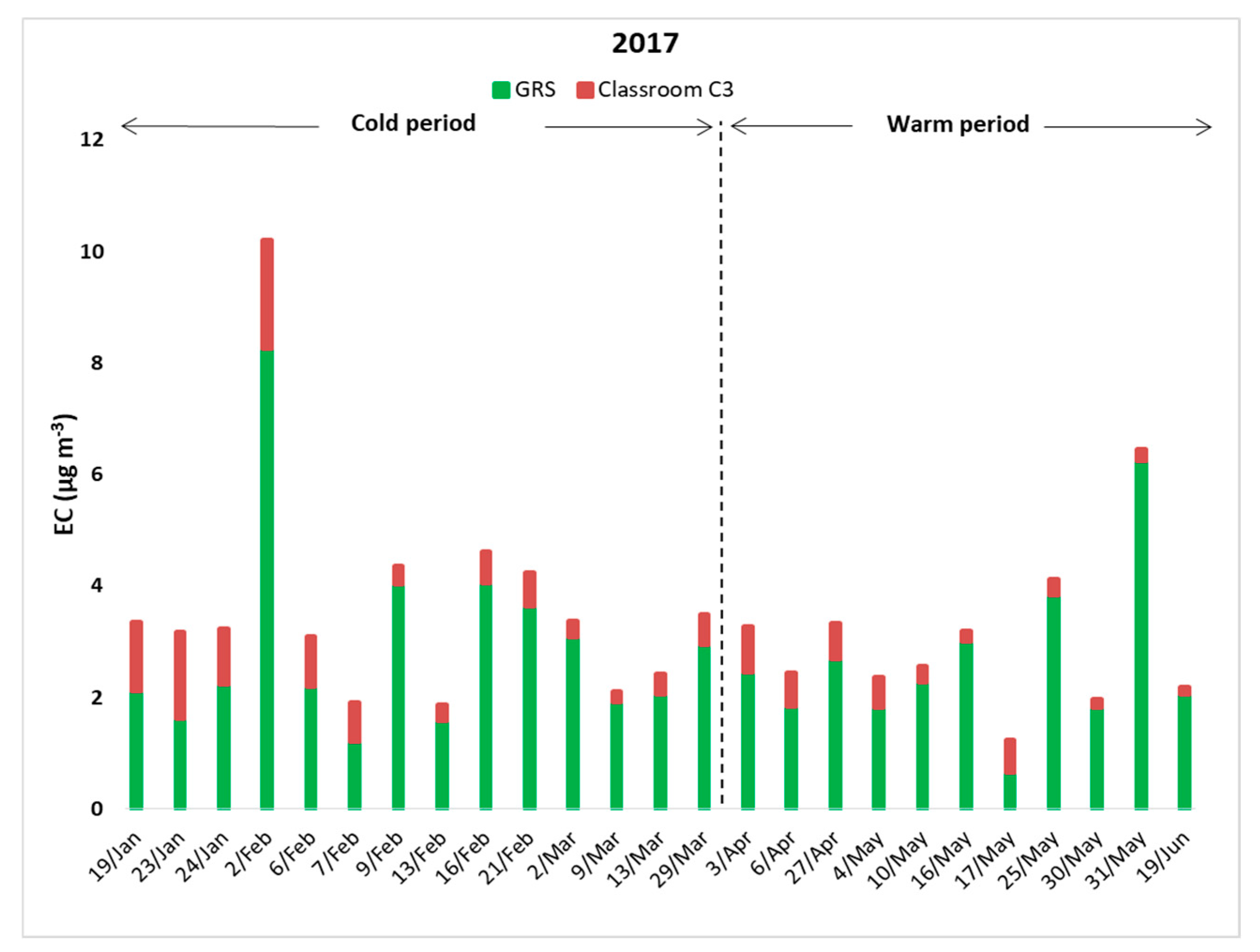
3.2. Organic and Elemental Carbon

Carbonaceous species are considered to be major components of PM₁₀. As Rajkumar and Chang [67] report, EC can be emitted as a product of incomplete combustion (e.g., diesel), while OC is mainly produced from anthropogenic or biogenic sources, either directly or formed in the atmosphere. In the present study, differences between internal and external concentrations of OC were found to be relatively balanced. More specifically, OC and EC accounted for 51.92% of total PM₁₀ within classroom C3 and 57.92% on the GRS, respectively, consistent with the results of Murillo et al. [68]. Mean concentrations, along with standard deviations, of indoor and outdoor OC and EC are summarized in

Table 3. Average values of organic carbon (OC) and elemental carbon (EC) within classroom C3 and on the GRS for the entire experimental period.

Carbonaceous Species	Classroom C3 (μg m−3)	GRS (μg m−3)
EC	0.60 ± 0.44	2.78 ± 1.62
OC	16.53 ± 7.70	16.67 ± 9.29

. In classroom C3, the average concentration of OC (16.53 ± 7.70 μg m⁻³), was slightly lower than the respective outdoor value (16.67 ± 9.29 μg m⁻³), while the mean value of EC on the GRS (2.78 ± 1.62 μg m⁻³) was almost 4.5 times higher than the respective indoor value (0.60 ± 0.44 μg m⁻³) due to local combustion activity. Figure 3 demonstrates that in 60% of the experimental days, OC concentrations in classroom C3 were elevated compared to outdoors (GRS). This result is related to resuspension of airborne coarse particles due to activities of pupils in the classroom (especially during the breaks), with possible internal emitting sources including small pieces of paper, skin debris and clothing fibers. These sources are also reported in the publication of Pegas et al. [69], referring to similar experiments in Portuguese schools. It should also be noted that closed windows seemed to be related with slightly higher concentrations of OC in classroom C3, as the mean internal value for the cold days was measured at 17.64 μg m⁻³. During the warmer days, the frequent opening of the windows led to a decreased mean value of OC (15.13 μg m⁻³). Additionally, during the cold period, for some cases, such as the 2nd of February, OC was found to be higher in the ambient environment than indoors, as expected. Elevated external concentrations of OC (such as the 31st of May) during the warm period could be related to the decomposition of plants on the GRS along with increased traffic emissions from nearby busy streets. For all measurements, the mean I/O ratio for the OC concentrations was found to be 1.2, indicating the importance of indoor activities (

Table 4. Average ratios of organic carbon (OC) and elemental carbon (EC) concentrations in different sampling sites.

Location	OC/EC Indoors	OC/EC Outdoor	OC I/O	EC I/O
Athens, Greece (This study)	34.6	6.4	1.2	0.3
Mira Loma, CA, USA [75]	7.4	5.0	1.4	0.8
Osaka, Japan [76]	1.1	0.9	1.1	0.8
Boston, MA, USA [77]	9.1	3.2	2.5	0.9
Baltimore, MD, USA [78]	24.3	10.8	1.8	0.8

).

Furthermore, Figure 4 illustrates that concentrations of EC on the GRS were higher than in classroom C3 for all experimental days. In addition, Table 4 shows that the average value of the I/O ratio was 0.3. These results indicate that EC concentrations were mostly linked to ambient sources such as exhaust emissions from vehicles or other combustion processes. More specifically, amid the cold period, mean concentration of EC on the GRS were found to be 2.92 μg m⁻³, and the respective values amid the warm period were 2.60 μg m⁻³. On the contrary, in classroom C3, EC demonstrated very low concentrations, ranging from 0.20 to 1.95 μg m⁻³ for the cold period and from 0.14 to 0.83 μg m⁻³ for the warm. It should also be mentioned that Spearman’s rho correlation coefficient between the outdoor OC and EC was 0.77 (p < 0.01), and, thus, OC and EC fractions may have originated from multiple emission sources and not only from a primary one, as Seleventi et al. [70] and Cao et al. [71] reported.

Moreover, the calculation of the OC/EC ratio is commonly used in order to investigate the presence of secondary organic aerosols (SOA), as according to Ho et al. [72] and Lonati et al. [73], when this ratio overcomes the value of 2, it corresponds to SOA formation and traffic emissions. Table 4 depicts such a behavior both indoors (34.6) and outdoors (6.4). Additionally, as Assimakopoulos et al. [74] report, for the case of fine particles (PM_2.5), higher values of OC/EC within the indoor environment compared to the outdoors demonstrates multiple possible indoor sources of OC concentrations. This is in accordance with the results of the present study (concerning PM₁₀), as the indoor OC/EC ratio was found to be almost 5.4 times higher than the respective outdoor value. Finally, the same table presents I/O and OC/EC ratios for the examined building, compared to other similar experimental campaigns. The higher ratio of indoor OC/EC may be due to a large variety of organic materials within the classroom C3.

3.3. Water-Soluble Anions

All PM₁₀ filter samples were analyzed for six different anionic components (chloride, nitrite, nitrate, bromide, phosphate and sulfate). Only chloride (Cl⁻), nitrate (NO₃⁻) and sulfate (SO₄²⁻) were traceable. The contribution of all measured anions accounted for 6.95% of the total PM₁₀ within classroom C3 and 11.06% on the GRS, respectively, which is similar to those detected in the study of Vargas et al. [79] in Bogota, Colombia. The significant contribution of the ambient emission sources (such as vehicles and heating systems from dwellings) to the indoor environment and, additionally, the presence of secondary inorganic particulates formed by the conversion of gaseous precursors were depicted. The most abundant anions were found to be SO₄²⁻ and NO₃⁻ followed by Cl⁻. This is in accordance with the study of Wang et al. [80]. Average concentrations along with standard deviations of indoor and outdoor anions per measuring period are summarized in

Table 5. Average values of PM₁₀ anionic components in different sampling sites.

Anions	Athens, Greece (This study)		Athens, Greece [81]		Aveiro, Portugal [69]		Chennai, India [82]
	Indoors (μg m−3)	Outdoors (μg m−3)	Indoors (μg m−3)	Outdoors (μg m−3)	Indoors (μg m−3)	Outdoors (μg m−3)	Indoors (μg m−3)
Cold period
Cl−	0.40 ± 0.25	0.57 ± 0.68	-	-	-	-	3.59 ± 1.20
NO3−	0.41 ± 0.20	1.41 ± 0.95	2.3 ± 1.80	3.8 ± 2.20	-	-	5.92 ± 1.67
SO42−	1.45 ± 0.82	1.78 ± 0.79	5.2 ± 1.40	6.7 ± 2.60	-	-	10.57 ± 2.92
Warm period
Cl−	0.28 ± 0.11	0.08 ± 0.10	-	-	0.67 ± 0.60	0.93 ± 1.05	3.65 ± 2.65
NO3−	0.48 ± 0.33	0.99 ± 0.72	-	-	1.02 ± 1.00	1.86 ± 1.40	4.23 ± 2.58
SO42−	1.57 ± 1.10	2.57 ± 1.18	-	-	1.27 ± 0.79	1.96 ± 1.25	12.13 ± 4.09

. In the same Table, the results of other similar experiments are also presented. It is obvious that anionic concentrations of the examined building were significantly decreased compared to measurements in different schools of the greater Athens area [81] and in a classroom close to a roadway within the city of Chennai, India [82]. However, the results are relatively comparable (especially for SO₄²⁻) with those of a Portuguese school in Aveiro [69] during the warm period.

In general, concentrations of Cl⁻ were relatively low both in the classroom C3 and the GRS during all experimental days. More precisely, during the cold period, mean indoor and outdoor concentrations of Cl⁻ were found to be 0.40 ± 0.25 μg m⁻³ and 0.57 ± 0.68 μg m⁻³, whereas amid the warm period they reached 0.28 ± 0.11μg m⁻³ and 0.08 ± 0.10 μg m⁻³, respectively. It is clear that for the cold days of the year, average concentration of Cl⁻ on the GRS seemed to be slightly higher than that for the indoors. The presence of comparatively higher Cl⁻ in the ambient environment is highly associated with transportation of marine aerosols from the sea, as Hassanvand et al. [83] and Tsitouridou et al. [84] report. However, during warm days, an opposite effect was observed, with mean internal concentration of Cl⁻ being 3.5 times higher than outdoors. Within the classroom, concentrations of Cl⁻ were influenced both by particle resuspension from human activities and the daily use of cleaning products after the end of lessons. The key role of detergents (such as residual chlorine particles) on Cl⁻ was also highlighted in the studies of Jaradat et al. [85], Park et al. [86] and Ashok et al. [87]. Thus, internal Cl⁻ seemed to originate mainly from indoor sources rather than be influenced from external penetration. This was also supported from Spearman’s rho concerning indoor and outdoor Cl⁻, which was calculated was 0.20 (p = 0.33) and demonstrated no significant correlation.

Regarding NO₃⁻, a different behavior compared to Cl⁻ was depicted. Concentrations were found to be relatively decreased for both periods. Average values of 0.41 ± 0.20 μg m⁻³ within the classroom C3 and 1.41 ± 0.95 μg m⁻³ on the GRS were measured for the cold days, whereas 0.48 ± 0.33 μg m⁻³ and 0.99 ± 0.72 μg m⁻³, respectively, were measured for the warmer days of the year. Elevated outdoor concentrations occurred for both periods but mainly during the cold period (almost 3.5 times higher than indoors), where apart from traffic load, there was a strong contribution from biomass burning from residential heating. Nevertheless, the influence of regionally transported external particles of NO₃⁻, which penetrate into the classroom, was obvious, as a significant Spearman correlation between the indoor and outdoor NO₃⁻ was observed for all experimental days with a correlation coefficient of 0.48 (p = 0.02). This is in accordance with the publications of Saraga et al. [88] and Ho et al. [89], which highlight that NO₃⁻ particles are strongly related to large scale regional transport processes, as they are formed in the atmosphere (SOA formation) mainly by the oxidation of nitrogen dioxide (NO₂), which is a primary product of combustion by vehicle exhausts, fireplaces and industrial activities.

Similar results were found for SO₄²⁻, which was the most abundant anionic element for both the indoor and outdoor environments compared to NO₃⁻ and Cl⁻. For all experimental days, higher ambient concentrations were recorded than those indoors. More specifically, amid the colder days, the mean value of SO₄²⁻ in classroom C3 was 1.45 ± 0.82μg m⁻³ and 1.78 ± 0.79 μg m⁻³ on the GRS, respectively. Interestingly, during the warm period, SO₄²⁻ mean concentrations were elevated in both experimental points (1.57 ± 1.10 μg m⁻³ and 2.57 ± 1.18μg m⁻³). A possible explanation could be the frequent regional transport episodes of airborne particles during the summer. As Cheng et al. [90], Souza et al. [91] and Kai et al. [92] report, sulfate anions are formed in the ambient environment as SOA, following heterogeneous or homogeneous sulfur dioxide (SO₂) reactions, which is emitted in the ambient environment as a primary product of combustion processes. The influence of ambient SO₄²⁻ to internal concentrations (penetration from windows and doors) was clearly significant, as for all PM₁₀ samples, Spearman’s rho correlation coefficient between the indoor and outdoor SO₄²⁻ was found to be 0.66 (p = 0.00). This is in agreement with the study of Saraga et al. [93], which highlighted that indoor sulfate mainly originated from external penetration rather than indoor sources.

3.4. Metals

The investigation of 16 elements (Al, As, Ba, Cd, Co, Cr, Cs, Cu, Fe, Mn, Ni, Pb, Sr, Tl, V and Zn), indoors and outdoors, depicted that their contribution to the total PM₁₀ was 22.28% in classroom C3 and 20.40% on the GRS, respectively. These results are comparable to those of Limbeck et al. [94], which refer to similar measurements in Vienna, Austria. It is important to note that for both the indoor and outdoor environments, principal earth crust elements Fe and Al prevailed, in consistency with the studies of Saraga et al., 2017 [66] and Di Vaio et al. [95]. More specifically, in classroom C3, Fe and Al accounted for the 9.55% and 8.68% of the total PM₁₀, followed by Zn (2.8%), Cr (0.46%), Ba (0.43%), Cu (0.28%), Ni (0.16%), Mn (0.15%), Sr (0.13%), V (0.12%), Pb (0.09%), Co (0.03%), As (0.01%), Cd (0.003%), Cs (0.001%) and Tl (0.0009%). Similar results were found on the GRS (Fe: 13.08%, Al: 4.04%, Zn: 1.55%, Cu: 0.35%, Ba: 0.33%, V: 0.25%, Mn: 0.21%, Cr: 0.18%, Ni: 0.14%, Pb: 0.14% Sr: 0.1%, Co: 0.01%, As: 0.01%, Cd: 0.004%, Cs: 0.001% and Tl: 0.0007%).

Among the investigated metals, Ni and Cd are regulated through WHO guidelines [96] with a maximum value of 1000 ng m^–3 for Ni and 5 ng m^–3 for Cd. Pb is regulated by the National Ambient Air Quality Standards (NAAQS) [97], with a value up to 150 ng m^–3 and by the 1999/30/EC European legislation directive [98], with a yearly limit of 500 ng m^–3. Because of their negative impact on humans, the 2004/107/EC directive [99] refers to annual limits of 20, 5 and 6 ng m^–3 for Ni, Cd and As, respectively (concerning PM₁₀). Indoor concentrations of As, Cd, Ni and Pb measured in classroom C3 was not found to overpass the respective limit values.

The calculation of EF (Equation (4)) for individual elements was implemented in order to investigate possible sources of indoor PM₁₀. Operationally, given the local variation in soil composition, an EF value exceeding 5 suggests that non-crustal sources contribute a significant fraction of the element [100]. An increase of the EF value provokes a subsequent increase to the contribution from non-crustal sources. Higher EF values implying anthropogenic activities of both the outdoor and indoor environment were determined sequentially for Cd, Zn, Cu, Pb, Ni and Cr, while the corresponding values for As and V were mainly of the outdoor environment (

Table 6. Enrichment factors (EFs) and indoor to outdoor concentration ratios (I/O) for the trace metals studied.

	EFindoor	EFoutdoor	I/O Ratio
Al	-	-	2.1
As	13	56	0.5
Ba	6.5	11	1.3
Cd	275	821	0.7
Co	17	14	2.5
Cr	47	39	2.6
Cs	2.4	4.0	1.3
Cu	95	253	0.8
Fe	2.2	6.5	0.7
Mn	1.5	4.4	0.7
Ni	32	62	1.1
Pb	51	170	0.6
Sr	3.7	6.4	1.2
Tl	9.4	17	1.2
V	12	52	0.5
Zn	307	470	1.4

). For all trace metals studied, excluding Cr and Co, EF values were found to be higher for the outdoor compared to the indoor environment, indicating that air infiltration constituted a significant factor of the enrichment of the classroom in trace metals, masking the original differences of indoor characteristics. This trend was confirmed in a relevant study regarding urban office areas in China [101]. High abundance of Cd and Cu was associated with traffic-related dust, high levels of As and Pb originating from coal combustion, whereas Zn was linked with combustion and vehicular emissions (mainly tire and brake wear), and Ni is typically known as an element linked with oil combustion, according to previous studies [102,103,104,105,106,107].

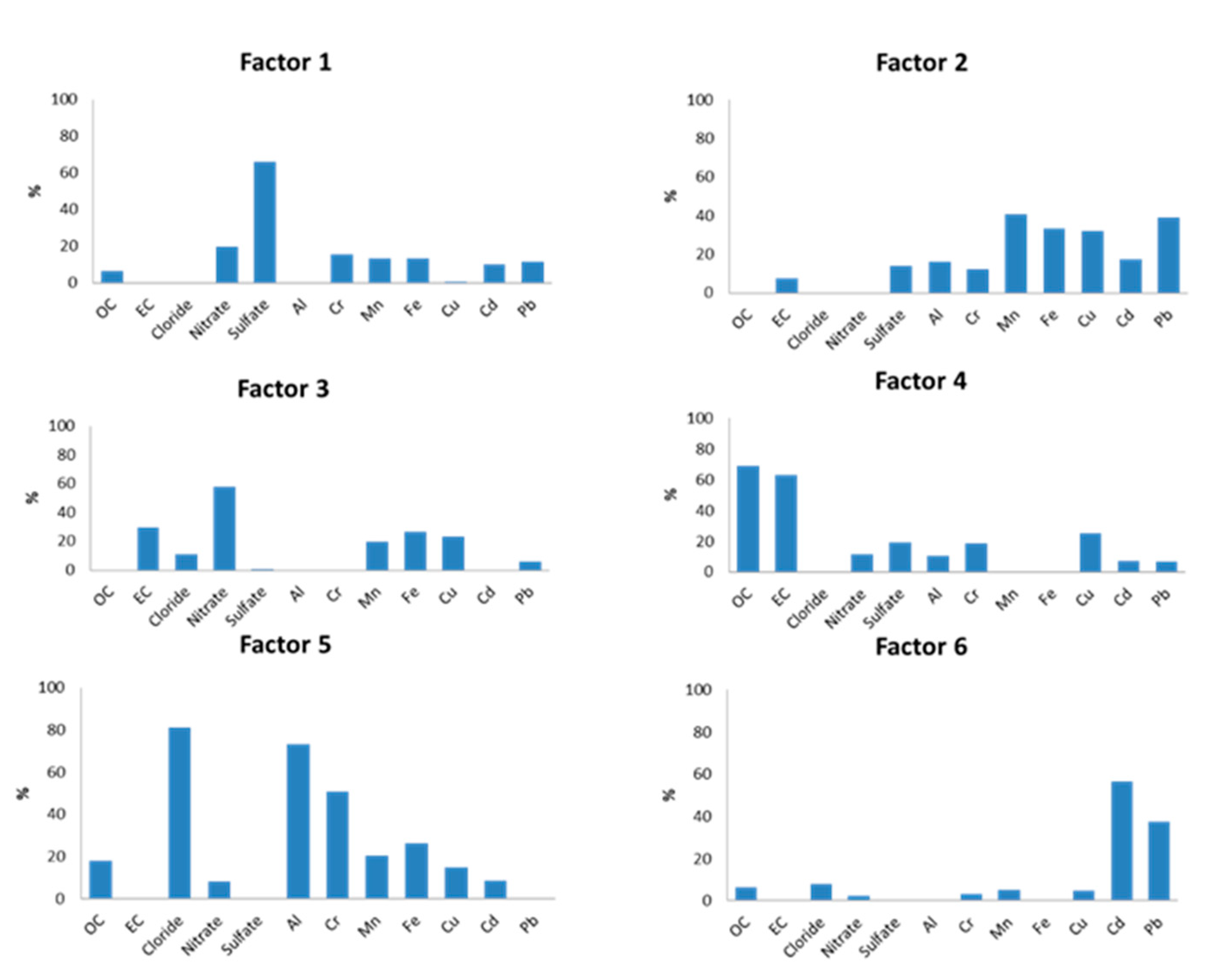
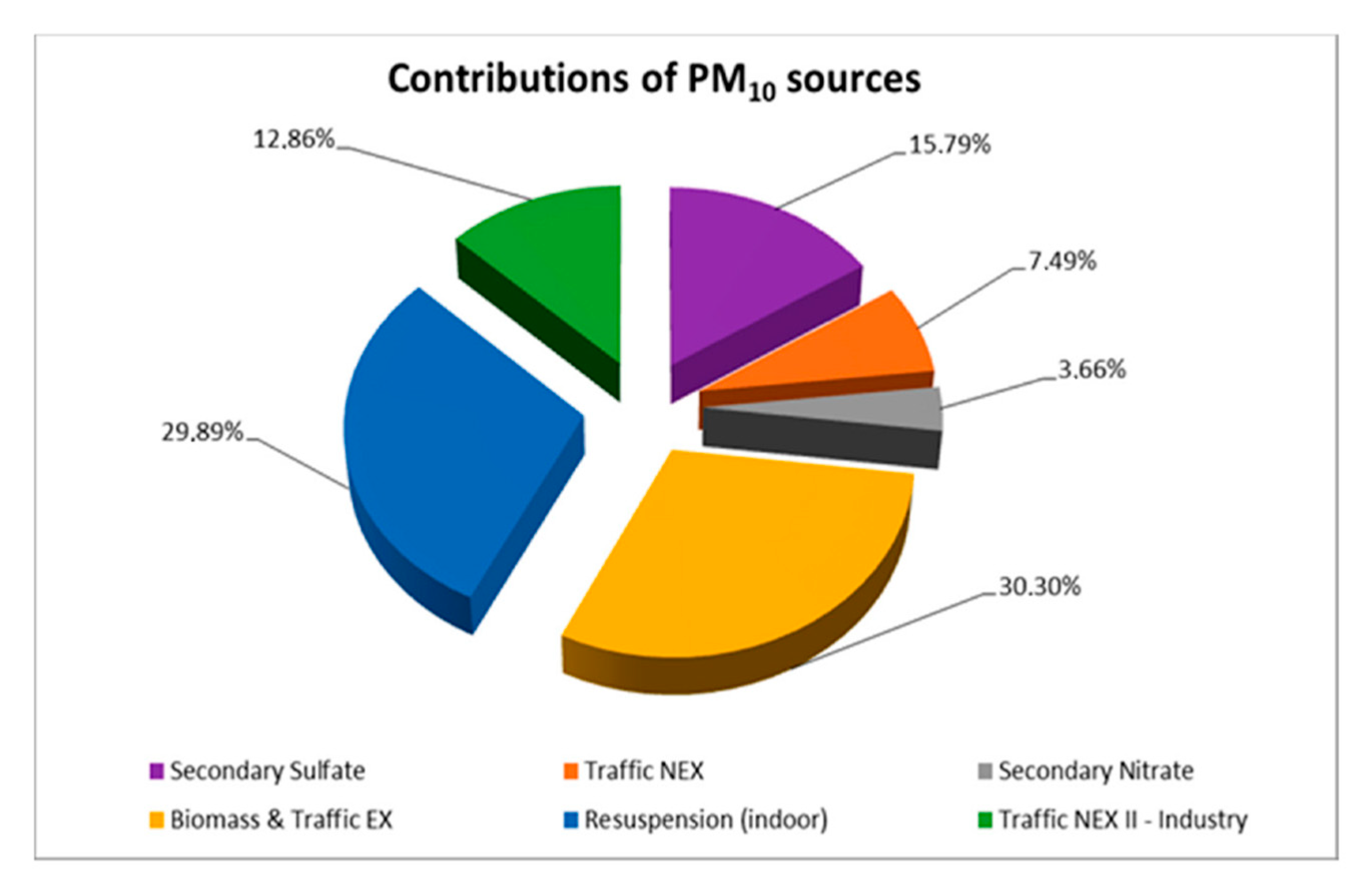
3.5. Source Apportionment Results

Application of the PMF model for both indoor and outdoor measurements (50 samples in total) resulted in six factors (sources) contributing to the measured PM₁₀. Figure 5 presents the contribution of each chemical element to the respective factor, while Figure 6 illustrates the contribution of each factor to the total mass of the measured PM₁₀.

The first factor corresponded to secondary sulfate particles, as it was characterized by 65.95% of SO₄²⁻ and lower percentages of organic fractions. The formation of secondary SO₄²⁻ in the atmosphere was due to the oxidation reactions of the primary pollutant SO₂ [108]. Therefore, this chemical component of PM₁₀ was mainly related to particle transport episodes from more distant sources [109,110]. This factor contributed 15.79% to the total of PM₁₀ sources.

The second factor was a mixture of dust from soil elements and car residues and was characterized as traffic non-exhaust (Traffic NEX). In particular, the contribution of earth crust elements Mn and Fe [111] in this factor reached 40.84% and 33.26%, respectively, while heavy metals such as Pb, Cu and Cd originating mainly from brakes and tires of vehicles on the road [112] contributed 38.84%, 31.91% and 17.55%. These particles were usually resuspended. This factor presented a low contribution to the total PM₁₀ mass concentration (7.49%).

The third factor was associated with the production of secondary NO₃⁻ (58.24%) with an additional contribution of EC (29.46%). This source was mainly due to primary NO₂, which was emitted into the atmosphere as a combustion product, transported over long distances and converted to NO₃⁻, as Han et al. [113] report. It is also worth noting that the existence of EC highlighted the presence of incomplete combustion products. This source demonstrated the lowest contribution to the total PM₁₀ (3.66%). It appeared mostly during the cold season, probably due to higher NO₂ emissions from cars and central heating from nearby dwellings, in combination with different meteorological conditions [114].

The fourth factor corresponded to a mixed source, as it was related to both vehicle exhaust and biomass burning (i.e., neighboring fireplaces (Biomass and Traffic EX)). In particular, the contributions of OC and EC to this factor were found to be 68.96% and 63.13%, respectively. The high percentage of OC combined with the elevated values of the OC/EC ratio in the external environment (Section 3.2) increased the probability of PM₁₀ emissions originating from biomass combustion processes, as the research of Waked et al. [115] highlighted. Moreover, as Yau et al. [116] and Cheng and Hu [117] reported, the high percentage of EC was associated with PM₁₀ emissions as products of incomplete combustion of gasoline or diesel in the engines of vehicles. This result was also strengthened by a 25.20% contribution of Cu found for this factor, a metal which is commonly associated with traffic emissions, as Loppi et al. [118] and Aksoy et al. [119]. mention. It is important to note that this factor presented the highest contribution to the total PM₁₀ sources with a percentage of 30.30%. This means that about 1/3 of the total measured particulate matter originated from this particular source. Additionally, seasonality also played a key role in the results, as amid the cold period, the contribution of the fireplaces from the neighboring dwellings was intense. On the contrary, during the warmer days, the external average concentration was mainly due to the exhaust of vehicles.

The fifth factor represented mainly indoor PM₁₀, which were resuspended in classroom C3 by the various activities of the students. The profile of this source included mostly Cl⁻ with a percentage of 81.19% and earth crust metals, specifically 73.38% of Al, 50.98% of Cr and 26.57% of Fe. Such a high percentage of chlorine anions was probably due to the daily use of chlorine (along with other detergents) by the cleaning service inside the classroom. Similar research in educational buildings [120,121] traced elevated Cl⁻ levels in indoor dust due to cleaning products such as chlorinated detergent and chlorinated water on the floor. Nevertheless, as Luo et al. [122] mentioned, the contribution of marine airborne particles from sea salt to the formation of chlorine anions (Cl⁻) was also possible, especially during the days that the south wind was prevailing. Furthermore, in accordance with Latif et al. [123], earth crust elements were commonly traced in the dust that settled on floors, desks and other surfaces of the classroom. The contribution of the fifth factor to the total PM₁₀ was the second largest (29.89%).

Lastly, the sixth factor contained airborne particles originating from the asphalt of the nearby streets. Heavy metals such as Cd and Pb demonstrated a strong contribution, with 56.43% and 37.33%, respectively. According to Lucarelli et al. [124], these particles appear from the friction of brakes, tires and other mechanical parts of vehicles passing by. However, this factor was not likely related to the second factor (Traffic NEX), as it contained a negligible amount of earth crust elements. Furthermore, the impact from small-scale industries (e.g., metallurgical activities) in the area could not be excluded. For that reason it was characterized as Traffic NEX II-Industry. This source contributed 12.86% of the total examined PM₁₀. The contribution of this factor in combination with that of the fourth factor highlight that local traffic load played a key role on the air quality levels of the school building.

In conclusion, the PMF receptor model demonstrated the profiles of six main factors as PM₁₀ sources in the indoor and outdoor environment of the school for the experimental period along with the contribution of each one of them to the total particulate mass. It seems that the dominant sources were vehicles (combustion and break and tire wear) and biomass burning during the colder days. Secondly, suspension of airborne particles in classroom C3 was also an important parameter that appeared mainly due to human activity and to frequent use of cleaning products. Finally, non-negligible sources of PM₁₀ were found to be SOA, originating from primary sulfate and nitrate transformations through long distance transport mechanisms.

4. Conclusions

The purpose of this paper is to investigate the levels and sources of indoor and outdoor PM₁₀ in a refurbished school building within an urban environment. As studies of IAQ in energy retrofitted educational buildings are limited, our research aims to fill this gap by providing results for the case of a preliminary school retaining a GRS, located in a densely built area of Athens, Greece. Additionally, this study enhances literature on the investigation of coarse airborne particle sources within a school microenvironment.

For this reason, an integrated 25-day experimental campaign took place from January to June 2017, divided into two periods (warm and cold). Measurements of PM₁₀ were implemented simultaneously on the GRS and in a classroom directly underneath the roof in order to compare mass concentration and chemical composition of the recorded particles between the two experimental sites. Some interesting conclusions are summarized as follows:

• The location of the school, both source and climate wise, played a major role in formulating its indoor and direct outdoor air quality, as traffic and residential heating were found to be the most important sources, together with resuspension.
• The existence of the GRS roof did not seem to have an impact on air quality. This is an expected result as this is the only building within many kilometers with vegetation on the roof. However, more experimental campaigns need to be implemented in order to estimate if a GRS can severely mitigate concentrations of particulate matter.
• Concentrations of PM₁₀ remained at relatively low levels and did not exceed the daily limit of 50 μg m⁻³, with a very few exceptions. Seasonal variations seem to affect results.
• During the cold period, higher PM₁₀ concentrations were measured on the GRS, probably due to biomass burning, central heating systems and traffic.
• On the other hand, during the warm period, PM₁₀ were found to be higher indoors, mainly because of resuspension of particles from human activities.
• No significant correlation between ambient and internal PM₁₀ was found depicting the importance of indoor activities.
• Concerning meteorological factors, elevated wind speed led to decreased levels of PM₁₀, while T and RH did not affect significantly the results.
• OC + EC accounted for the larger percentage (51.92% indoors and 57.92% outdoors) of total measured PM₁₀.
• Closed windows were related to elevated OC levels within the classroom because of resuspension.
• On the contrary, EC concentrations were measured higher on the GRS, the I/O ratio being notably lower than unity, since EC is strongly associated with outdoor sources such as combustion processes. The calculation of the OC/EC ratio showed higher values indoors, depicting the influence of multiple possible indoor sources of organic materials, such as small pieces of paper, skin debris and clothing fibers.
• The investigation of water soluble anions demonstrated that the use of cleaning products as well as resuspension and infiltration of SOA dominated the indoor air quality, while marine aerosols and SOA dominated the outdoor air quality.
• The most abundant metals in both experimental areas were found to be the earth crust elements Fe and Al, while penetration of ambient air seemed to play a key role in the enrichment of the indoor environment in trace metals.
• Source apportionment results highlighted six main factors as emission sources of PM₁₀ both indoors and outdoors. It seems that the largest percentage of contribution is related to combustion products from vehicles and biomass burning. The second most important source of pollution is associated with resuspension of particles in the classroom C3 due to activities of pupils. Furthermore, the contribution of asphalt residues from the brakes and tires of the vehicles is also important. Finally, non-negligible external sources of PM₁₀ were found to be sulfate and nitrate SOA, mainly originating from remote sources.

This study aims to enhance a general plan for the improvement of air quality in schools, where possible. As the main source of PM₁₀ was found to be mainly the traffic load and combustion processes from local heating systems (during winter), one may suggest moving the school building to an area with cleaner air, where those emission sources during class hours could be limited. In addition, as the second most important source was resuspension of particles from indoor human activity, it is of great importance to use eco-friendly detergents, to design and install a brand new mechanical ventilation system and maybe to mitigate the number of pupils in each classroom in order to reduce viral load, such as COVID-19 recently.

Future research should aim at in situ measurements and a source apportionment approach in order to investigate IAQ levels within educational buildings in order to secure healthy conditions for the students and staff. Retrofitting interventions within a building (and mainly in schools) should always be accompanied by acceptable IAQ levels.

References

1. Annesi-Maesano, I.; Hulin, M.; Lavaud, F.; Raherison, C.; Kopferschmitt, C.; de Blay, F.; André Charpin, D.; Denis, C. Poor air quality in classrooms related to asthma and rhinitis in primary school children of the French 6 Cities Study. Thorax 2012, 67, 682–688. [Google Scholar] [CrossRef] [Green Version]
2. Faustman, E.M.; Faustman, E.M.; Silbernagel, S.M.; Fenske, R.A.; Burbacher, T.M.; Ponce, R.A. Mechanisms underlying Children’s susceptibility to environmental toxicants. Environ. Health Perspect. 2000, 108, 13–21. [Google Scholar] [CrossRef] [Green Version]
3. Godoi, R.H.M.; Avigo, D., Jr.; Campos, V.P.; Tavares, T.M.; de Marchi, M.M.R.; Grieker, R.V.; Godoi, A.F.L. Indoor air quality assessment of elementary schools in Curitiba, Brazil. Water Air Soil Pollut. 2009, 9, 171–177. [Google Scholar] [CrossRef]
4. Madureira, J.; Paciência, I.; Fernandes, E.O. Levels and indoor–outdoor relationships of size-specific particulate matter in naturally ventilated Portuguese schools. J. Toxicol. Environ. Health A 2012, 75, 1423–1436. [Google Scholar] [CrossRef]
5. Rovelli, S.; Cattaneo, A.; Nuzzi, C.P.; Spinazzè, A.; Piazza, S.; Carrer, P.; Cavallo, D.M. Airborne particulate matter in school classrooms of northern Italy. Int. J. Environ. Res. Public Health 2014, 11, 1398–1421. [Google Scholar] [CrossRef] [Green Version]
6. Peters, A.; Perz, S.; Döring, A.; Stieber, J.; König, W.; Wichmann, H.E. Activation of the autonomic nervous system and blood coagulation in association with an air pollution episode. Inhal. Toxicol. 2000, 12, 51–61. [Google Scholar] [CrossRef]
7. Samet, J.M.; Dominici, F.; Curriero, F.C.; Coursac, I.; Zeger, S.L. Fine particulate air pollution and mortality in 20 US cities, 1987–1994. N. Engl. J. Med. 2000, 343, 1742–1749. [Google Scholar] [CrossRef]
8. Le Tertre, A.; Medina, S.; Samoli, E.; Forsberg, B.; Michelozzi, P.; Boumghar, A.; Vonk, J.M.; Bellini, A.; Atkinson, R.; Ayres, J.G.; et al. Short-term effects of particulate air pollution on cardiovascular diseases in eight European cities. J. Epidemiol. Community Health 2002, 56, 773. [Google Scholar] [CrossRef]
9. Alves, C.; Duarte, M.; Ferreira, M.; Alves, A.; Almeida, A.; Cunha, Â. Air quality in a school with dampness and mould problems. Air Qual. Atmos. Health 2016, 9, 107–115. [Google Scholar] [CrossRef]
10. Lee, S.C.; Chang, M. Indoor and outdoor air quality investigation at schools in Hong Kong. Chemosphere 2000, 41, 109–113. [Google Scholar] [CrossRef]
11. Madureira, J.; Paciencia, I.; Rufo, J.; Ramos, E.; Barros, H.; Teixeira, J.P.; Fernandes, E.D. Indoor air quality in schools and its relationship with children’s respiratory symptoms. Atmos. Environ. 2015, 118, 145–156. [Google Scholar] [CrossRef] [Green Version]
12. Rufo, J.C.; Madureira, J.; Paciencia, I.; Aguiar, L.; Teixeira, J.P.; Moreira, A.; De Oliveira Fernandes, E. Indoor air quality and atopic sensitization in primary schools: A follow-up study. Porto BioMed. J. 2016, 1, 142–146. [Google Scholar] [CrossRef] [PubMed] [Green Version]
13. Stabile, L.; Dell’Isola, M.; Russi, A.; Massimo, A.; Buonanno, G. The effect of natural ventilation strategy on indoor air quality in schools. Sci. Total Environ. 2017, 595, 894–902. [Google Scholar] [CrossRef] [PubMed]
14. Mainka, A.; Brąagoszewska, E.; Kozielska, B.; Pastuszka, J.S.; Zajusz-Zubek, E. Indoor air quality in urban nursery schools in Gliwice, Poland: Analysis of the case study. Atmos. Pollut. Res. 2015, 6, 1098–1104. [Google Scholar] [CrossRef]
15. Canha, N.; Mandin, C.; Ramalho, O.; Wyart, G.; Ribéron, J.; Dassonville, C.; Hänninen, O.; Almeida, S.M.; Derbez, M. Assessment of ventilation and indoor air pollutants in nursery and elementary schools in France. Indoor Air 2016, 26, 350–365. [Google Scholar] [CrossRef]
16. Janssen, N.A.H.; Brunekreef, B.; van Vliet, P.; Aarts, F.; Meliefste, K.; Harssema, H.; Fischer, P. The relationship between air pollution from heavy traffic and allergic sensitization, bronchial hyperresponsiveness, and respiratory symptoms in Dutch schoolchildren. Environ. Health Perspect. 2003, 111, 1512–1518. [Google Scholar] [CrossRef] [Green Version]
17. Oeder, S.; Dietrich, S.; Weichenmeier, I.; Schober, W.; Pusch, G.; Jörres, R.A.; Schierl, R.; Nowak, D.; Fromme, H.; Behrendt, H.; et al. Toxicity and elemental composition of particulate matter from outdoor and indoor air of elementary schools in Munich, Germany. Indoor Air 2012, 22, 148–158. [Google Scholar] [CrossRef]
18. Rivas, I.; Viana, M.; Moreno, T.; Pandolfi, M.; Amato, F.; Reche, C.; Bouso, L.; Àlvarez-Pedrerol, M.; Alastuey, A.; Sunyer, J.; et al. Child exposure to indoor and outdoor air pollutants in schools in Barcelona, Spain. Environ. Int. 2014, 69, 200–212. [Google Scholar] [CrossRef] [Green Version]
19. Meyer, H.W.; Suadicani, P.; Nielsen, P.A.; Sigsgaard, T.; Gyntelberg, F. Moulds in floor dust—A particular problem in mechanically ventilated, rooms? A study of adolescent schoolboys under the Danish moulds in buildings program. Scand. J. Work Environ. Health 2011, 37, 332–340. [Google Scholar] [CrossRef] [Green Version]
20. Krugly, E.; Martuzevicius, D.; Sidaraviciute, R.; Ciuzas, D.; Prasauskas, T.; Kauneliene, V.; Stasiulaitiene, I.; Kliucininkas, L. Characterization of Particulate and Vapor Phase Polycyclic Aromatic Hydrocarbons in Indoor and Outdoor Air of Primary Schools. Atmos. Environ. 2014, 82, 298–306. [Google Scholar] [CrossRef]
21. Szoboszlai, Z.; Furu, E.; Angyal, A.; Szikszai, Z.; Kertesz, Z. Investigation of indoor aerosols collected at various educational institutions in Debrecen, Hungary. X-Ray Spectrom. 2011, 40, 176–180. [Google Scholar] [CrossRef]
22. Braniš, M.; Řezáčová, P.; Domasová, M. The effect of outdoor air and indoor human activity on mass concentrations of PM10, PM2.5, and PM1 in a classroom. Environ Res. 2005, 99, 143–149. [Google Scholar] [CrossRef] [PubMed]
23. Allaerts, K.; Koussa, J.A.; Desmedt, J.; Salenbien, R. Improving the energy efficiency of ground-source heat pump systems in heating dominated school buildings: A case study in Belgium. Energy Build. 2017, 138, 559–568. [Google Scholar] [CrossRef]
24. Goyal, R.G.; Khare, M. Indoor-outdoor concentrations of RSPM in classroom of a naturally ventilated school building near an urban traffic roadway. Atmos. Environ. 2009, 43, 6026–6038. [Google Scholar] [CrossRef]
25. Yang, W.; Sohn, J.; Kim, J.; Son, B.; Park, J. Indoor air quality investigation according to age of the school buildings in Korea. J. Environ. Manag. 2009, 90, 348–354. [Google Scholar] [CrossRef] [PubMed]
26. Ismail, M.; Sofian, N.Z.M.; Abdullah, A.M. Indoor air quality in selected samples of primary schools in Kuala Terengganu, Malaysia. Environ. Asia 2010, 3, 103–108. [Google Scholar] [CrossRef]
27. Ma, F.; Zhan, C.; Xu, X. Investigation and evaluation of winter indoor air quality of primary schools in severe cold weather areas of China. Energies 2019, 12, 1602. [Google Scholar] [CrossRef] [Green Version]
28. Abdel-Salam, M.M.M. Investigation of indoor air quality at urban schools in Qatar. Indoor Built Environ. 2017, 28, 278–288. [Google Scholar] [CrossRef]
29. Petronella, S.; Thomas, R.; Stone, J.; Goldblum, R.; Brooks, E. Clearing the air: A model for investigating indoor air quality in Texas schools. J. Environ. Health 2005, 67, 35–42. [Google Scholar] [PubMed]
30. Levetin, E.; Shaughnessy, R.; Fisher, E.; Ligman, B.; Harrison, J.; Brennan, T. Indoor air quality in schools: Exposure to fungal allergens. Aerobiologia 1995, 11, 27–34. [Google Scholar] [CrossRef]
31. Godwin, C.; Batterman, S. Indoor air quality in Michigan schools. Indoor Air 2007, 17, 109–121. [Google Scholar] [CrossRef] [Green Version]
32. Shendell, D.G.; Prill, R.; Fisk, W.J.; Apte, M.G.; Blake, D.; Faulkner, D. Associations between classroom CO2 concentrations and student attendance in Washington and Idaho. Indoor Air 2004, 14, 333–341. [Google Scholar] [CrossRef]
33. Majd, E.; McCormack, M.; Davis, M.; Curriero, F.; Berman, J.; Connolly, F.; Leaf, P.; Rule, A.; Green, T.; Clemons-Erby, D.; et al. Indoor air quality in inner-city schools and its associations with building characteristics and environmental factors. Environ. Res. 2019, 170, 83–91. [Google Scholar] [CrossRef]
34. Guo, H.; Morawska, L.; He, C.; Zhang, Y.L.; Ayoko, G.; Cao, M. Characterization of particle number concentrations and PM2.5 in a school: Influence of outdoor air pollution on indoor air. Environ. Sci. Pollut. Res. Int. 2010, 17, 1268–1278. [Google Scholar] [CrossRef] [Green Version]
35. Avigo, D.; Godoi, A.F.L.; Janissek, P.R.; Makarovska, Y.; Krata, A.; Potgieter-Vermaak, S.; Alfoldy, B.; Grieken, R.V.; Godoi, R.H.M. Particulate Matter Analysis at Elementary Schools in Curitiba, Brazil. Anal. Bioanal. Chem. 2008, 391, 1459–1468. [Google Scholar] [CrossRef]
36. Mustapha, B.A.; Blangiardo, M.; Briggs, D.J.; Hansell, A.L. Traffic air pollution and other risk factors for respiratory illness in schoolchildren in the Niger-delta region of Nigeria. Environ. Health Perspect. 2011, 119, 1478–1482. [Google Scholar] [CrossRef]
37. Diapouli, E.; Chaloulakou, A.; Spyrellis, N. Levels of ultrafine particles in different micro-environments—Implications to children exposure. Sci. Total Environ. 2007, 388, 128–136. [Google Scholar] [CrossRef]
38. Chaloulakou, A.; Mavroidis, I. Comparison of indoor and outdoor concentrations of CO at a public school. Evaluation of an indoor air quality model. Atmos. Environ. 2002, 36, 1769–1781. [Google Scholar] [CrossRef]
39. Siskos, P.A.; Bouba, K.E.; Stroubou, A.P. Determination of selected pollutants and measurement of physical parameters for the evaluation of indoor air quality in school buildings in Athens, Greece. Indoor Built Environ. 2001, 10, 185–192. [Google Scholar] [CrossRef]
40. Synnefa, A.; Polichronaki, E.; Papagiannopoulou, E.; Santamouris, M.; Mihalakakou, G.; Doukas, P.; Siskos, P.A.; Bakeas, E.; Dremetsika, A.; Geranios, A.; et al. An experimental investigation of the indoor air quality in fifteen school buildings in Athens. Int. J. Vent. 2003, 2, 185–201. [Google Scholar] [CrossRef]
41. Dorizas, P.V.; Kapsanaki-Gotsi, E.; Assimakopoulos, M.N.; Santamouris, M. Particulate matter and airborne fungi concentrations in schools in Athens. In Proceedings of the 11th International Conference on Meteorology, Climatology and Atmospheric Physics (COMECAP 2012), Athens, Greece, 29 May–1 June 2012. [Google Scholar]
42. Dimoudi, A.; Kostarela, P. Energy monitoring and conservation potential in school buildings in the C’ climatic zone of Greece. Renew. Energy 2009, 34, 289–296. [Google Scholar] [CrossRef]
43. Dascalaki, E.G.; Sermpetzoglou, V.G. Energy performance and indoor environmental quality in Hellenic schools. Energy Build. 2011, 43, 718–727. [Google Scholar] [CrossRef]
44. Kalimeri, K.K.; Saraga, D.E.; Lazaridis, V.D.; Legkas, N.A.; Missia, D.A.; Tolis, E.I.; Bartzis, J.G. Indoor air quality investigation of the school environment and estimated health risks: Two-season measurements in primary schools in Kozani, Greece. Atmos. Pollut. Res. 2016, 7, 1128–1142. [Google Scholar] [CrossRef]
45. Kim, J.; Hong, T.; Koo, C. Economic and environmental evaluation model for selecting the optimum design of green roof systems in elementary schools. Environ. Sci. Technol. 2012, 46, 8475–8483. [Google Scholar] [CrossRef]
46. Hong, T.H.; Kim, J.M.; Koo, C.W. LCC and LCCO2 analysis of green roofs in elementary schools with energy saving measures. Energy Build. 2012, 45, 229–239. [Google Scholar] [CrossRef]
47. Perini, K. Retrofitting with vegetation recent building heritage applying a design tool—The case study of a school building. Front. Archit. Res. 2013, 2, 267–277. [Google Scholar] [CrossRef] [Green Version]
48. Ascione, F.; Bianco, N.; De Masi, R.F.; De Rossi, F.; Vanoli, G.P. Mitigating the cooling need and improvement of indoor conditions in Mediterranean educational buildings, by means of green roofs. Results of a case study. J. Phys. Conf. Ser. 2015, 655, 12027. [Google Scholar] [CrossRef] [Green Version]
49. Yang, J.; Yu, Q.; Gong, P. Quantifying air pollution removal by green roofs in Chicago. Atmos. Environ. 2008, 42, 7266–7273. [Google Scholar] [CrossRef]
50. Currie, B.A.; Bass, B. Estimates of air pollution mitigation with green plants and green roofs using the UFORE model. Urban Ecosyst. 2008, 11, 409–422. [Google Scholar] [CrossRef]
51. Speak, A.F.; Rothwell, J.J.; Lindley, S.J.; Smith, C.L. Urban particulate pollution reduction by four species of green roof vegetation in a UK city. Atmos. Environ. 2012, 61, 283–293. [Google Scholar] [CrossRef]
52. EN 12341:2014—Ambient Air—Standard Gravimetric Measurement Method for the Determination of the PM10 or PM2.5 Mass Concentration of Suspended Particulate Matter; European Committee for Standardization: Brussels, Belgium, 2014.
53. Popovicheva, O.B.; Engling, G.; Diapouli, E.; Saraga, D.; Persiantseva, N.M.; Timofeev, M.A.; Kireeva, E.D.; Shonija, N.K.; Chen, S.-H.; Nguyen, D.-L.; et al. Impact of smoke intensity on size-resolved aerosol composition and microstructure during the biomass burning season in northwest Vietnam. Aerosol Air Qual. Res. 2016, 16, 2635–3654. [Google Scholar] [CrossRef]
54. Romanazzi, V.; Casazza, M.; Malandrino, M.; Maurino, V.; Piano, A.; Schilirò, T.; Gilli, G. PM10 size distribution of metals and environmental-sanitary risk analysis in the city of Torino. Chemosphere 2014, 112, 210–216. [Google Scholar] [CrossRef] [Green Version]
55. Paatero, P. Least squares formulation of robust nonnegative factor analysis. Chemom. Intell. Lab. Syst. 1997, 37, 23–35. [Google Scholar] [CrossRef]
56. Liao, H.-T.; Chou, C.C.-K.; Chow, J.C.; Watson, J.G.; Hopke, P.K.; Wu, C.-F. Source and risk apportionment of selected VOCs and PM2.5 species using partially constrained receptor models with multiple time resolution data. Environ. Pollut. 2015, 205, 121–130. [Google Scholar] [CrossRef]
57. Polissar, A.; Hopke, P.; Poirot, R. Atmospheric aerosol over Vermont: Chemical composition and sources. Environ. Sci. Technol. 2001, 35, 4604–4621. [Google Scholar] [CrossRef]
58. Rudnick, R.L.; Gao, S. Composition of the continental crust. In Treatise on Geochemistry; Elsevier Science: Amsterdam, The Netherlands, 2003; pp. 1–64. [Google Scholar]
59. European Air Quality Standards. Available online: https://ec.europa.eu/environment/air/quality/standards.htm (accessed on 24 January 2020).
60. Fameli, K.M.; Assimakopoulos, V.D. The new open Flexible Emission Inventory for Greece and the Greater Athens Area (FEI-GREGAA): Account of pollutant sources and their importance from 2006 to 2012. Atmos. Environ. 2016, 137, 17–37. [Google Scholar] [CrossRef]
61. Fameli, K.M.; Assimakopoulos, V.D. Development of a road transport emission inventory for Greece and the Greater Athens Area: Effects of important parameters. Sci. Total Environ. 2015, 505, 770–786. [Google Scholar] [CrossRef] [Green Version]
62. Agudelo-Castañeda, D.M.; Teixeira, E.C.; Braga, M.; Rolim, S.B.A.; Silva, L.F.O.; Beddows, D.C.S.; Harrison, R.M.; Querol, X. Cluster analysis of urban ultrafine particles size distributions. Atmos. Pollut. Res. 2019, 10, 45–52. [Google Scholar] [CrossRef]
63. Soleimanian, E.; Taghvaee, S.; Mousavi, A.; Sowlat, M.H.; Hassanvand, M.S.; Yunesian, M.; Naddafi, K.; Sioutas, C. Sources and Temporal Variations of Coarse Particulate Matter (PM) in Central Tehran, Iran. Atmosphere 2019, 10, 291. [Google Scholar] [CrossRef] [Green Version]
64. Zwoździak, A.; Sówka, I.; Krupińska, B.; Zwoździak, J.; Nych, A. Infiltration or indoor sources as determinants of the elemental composition of particulate matter inside a school in Wrocław, Poland? Build. Environ. 2013, 66, 173–180. [Google Scholar] [CrossRef]
65. Karar, K.; Gupta, A.K. Seasonal variations and chemical characterization of ambient PM10 at residential and industrial sites of an urban region of Kolkata (Calcutta), India. Atmos. Res. 2006, 81, 36–53. [Google Scholar] [CrossRef]
66. Saraga, D.; Maggos, T.; Sadoun, E.; Fthenou, E.; Hassan, H.; Tsiouri, V.; Karavoltsos, S.; Sakellari, A.; Vasilakos, C.; Kakosimos, K. Chemical characterization of indoor and outdoor particulate matter (PM2.5, PM10) in Doha, Qatar. Aerosol Air Qual. Res. 2017, 17, 1156–1168. [Google Scholar] [CrossRef] [Green Version]
67. Rajkumar, W.S.; Chang, A.S. Suspended particulate concentrations along the East-West-Corridor, Trinidad, West Indies. Atmos. Environ. 2000, 34, 1181–1197. [Google Scholar] [CrossRef]
68. Murillo, J.H.; Roman, S.R.; Rojas Marin, J.F.; Campos, R.; Blanco, J.S.; Cardenas, G.B.; Gibson Baumgardner, D. Chemical characterization and source apportionment of PM10 and PM2.5 in the metropolitan area of Costa Rica, Central America. Atmos. Pollut. Res. 2013, 4, 181–190. [Google Scholar] [CrossRef] [Green Version]
69. Pegas, P.N.; Nunes, T.; Alves, C.; Silva, J.R.; Vieira, S.L.A.; Caseiro, A.; Pio, C.A. Indoor and outdoor characterisation of organic and inorganic compounds in city centre and suburban elementary schools of Aveiro, Portugal. Atmos. Environ. 2012, 55, 80–89. [Google Scholar] [CrossRef]
70. Seleventi, M.K.; Saraga, D.E.; Helmis, C.G.; Bairachtari, K.; Vasilakos, C.; Maggos, T. PM2.5 indoor/outdoor relationship and chemical composition in ions and OC/EC in an apartment in the center of Athens. Fresenius Environ. Bull. 2012, 21, 3177–3183. [Google Scholar]
71. Cao, J.J.; Huang, H.; Lee, S.C.; Chow, J.C.; Zou, C.W.; Ho, K.F.; Watson, J.G. Indoor/Outdoor Relationships for Organic and Elemental Carbon in PM2.5 at Residential Homes in Guangzhou, China. Aerosol Air Qual. Res. 2012, 12, 902–910. [Google Scholar] [CrossRef] [Green Version]
72. Ho, K.F.; Cao, J.J.; Harrison, R.M.; Lee, S.C.; Bau, K.K. Indoor/outdoor relationships of organic carbon (OC) and elemental carbon (EC) in PM2.5 in roadside environment of Hong Kong. Atmos. Environ. 2004, 38, 6327–6335. [Google Scholar] [CrossRef]
73. Lonati, G.; Ozgen, S.; Giugliano, M. Primary and secondary carbonaceous species in PM2.5 samples in Milan (Italy). Atmos. Environ. 2007, 41, 4599–4610. [Google Scholar] [CrossRef]
74. Assimakopoulos, V.D.; Bekiari, T.; Pateraki, S.; Maggos, T.; Stamatis, P.; Nicolopoulou, P.; Assimakopoulos, M.N. Assessing personal exposure to PM using data from an integrated indoor-outdoor experiment in Athens-Greece. Sci. Total Environ. 2018, 636, 1303–1320. [Google Scholar] [CrossRef]
75. Na, K.; Cocker, D.R. Organic and Elemental Carbon Concentrations in Fine Particulate Matter in Residences, Schoolrooms, and Outdoor Air in Mira Loma, California. Atmos. Environ. 2006, 39, 3325–3333. [Google Scholar] [CrossRef]
76. Funasaka, K.; Miyazaki, T.; Tsuruho, K.; Tamura, K.; Mizuno, T.; Kuroda, K. Relationship between indoor and outdoor carbonaceous particulates in roadside households. Environ. Pollut. 2000, 110, 127–134. [Google Scholar] [CrossRef]
77. Long, C.M.; Suh, H.H.; Koutrakis, P. Characterization of indoor particle sources using continuous mass and size monitors. J. Air Waste Manag. Assoc. 2000, 50, 1236–1250. [Google Scholar] [CrossRef] [PubMed]
78. Landis, M.S.; Norris, G.A.; Williams, R.W.; Weinstein, J.P. Personal exposures to PM2.5 mass and trace elements in Baltimore, MD, USA. Atmos. Environ. 2001, 35, 6511–6524. [Google Scholar] [CrossRef]
79. Vargas, F.; Rojas, N.Y.; Pachon, J.E.; Russell, A.G. PM10 characterization and source apportionment at two residential areas in Bogota. Atmos. Pollut. Res. 2012, 3, 72–80. [Google Scholar] [CrossRef] [Green Version]
80. Wang, Q.; Cao, J.; Shen, Z.; Tao, J.; Xiao, S.; Luo, L.; He, Q.; Tang, X. Chemical characteristics of PM2.5 during dust storms and air pollution events in Chengdu, China. Particuology 2012, 11, 70–77. [Google Scholar] [CrossRef]
81. Diapouli, E.; Chaloulakou, A.; Mihalopoulos, N.; Spyrellis, N. Indoor and outdoor PM mass and number concentrations at schools in the Athens area. Environ. Monit. Assess. 2008, 136, 13–20. [Google Scholar] [CrossRef] [PubMed]
82. Chithra, V.S.; Shiva Nagendra, S.M. Chemical and morphological characteristics of indoor and outdoor particulate matter in an urban environment. Atmos. Environ. 2013, 77, 579–587. [Google Scholar] [CrossRef]
83. Hassanvand, M.S.; Naddafi, K.; Faridi, S.; Arhami, M.; Nabizadeh, R.; Sowlat, M.H.; Pourpak, Z.; Rastkari, N.; Momeniha, F.; Kashani, H.; et al. Indoor/outdoor relationships of PM10, PM2.5, and PM1 mass concentrations and their water-soluble ions in a retirement home and a school dormitory. Atmos. Environ. 2014, 82, 375–382. [Google Scholar] [CrossRef]
84. Tsitouridou, R.; Voutsa, D.; Kouimtzis, T. Ionic composition of PM10 in the area of Thessaloniki, Greece. Chemosphere 2003, 52, 883–891. [Google Scholar] [CrossRef]
85. Jaradat, Q.M.; Momani, K.A.; Jbarah, A.-A.Q.; Massadeh, A. Inorganic analysis of dust fall and office dust in an industrial area of Jordan. Environ. Res. 2004, 96, 139–144. [Google Scholar] [CrossRef] [PubMed]
86. Park, D.; Oh, M.; Yoon, Y.; Park, E.; Lee, K. Source identification of PM10 pollution in subway passenger cabins using positive matrix factorization. Atmos. Environ. 2012, 49, 180–185. [Google Scholar] [CrossRef]
87. Ashok, V.; Gupta, T.; Dubey, S.; Jat, R. Personal exposure measurement of students to various microenvironments inside and outside the college campus. Environ. Monit. Assess. 2014, 186, 735–750. [Google Scholar] [CrossRef] [PubMed]
88. Saraga, D.E.; Makrogkika, A.; Karavoltsos, S.; Sakellari, A.; Diapouli, E.; Eleftheriadis, K.; Vasilakos, C.; Helmis, C.; Maggos, T. A pilot investigation of PM indoor/outdoor mass concentration and chemical analysis during a period of extensive fireplace use in Athens. Aerosol Air Qual. Res. 2015, 15, 2485–2495. [Google Scholar] [CrossRef] [Green Version]
89. Ho, K.F.; Lee, S.C.; Chan, C.K.; Yu, J.C.; Chow, J.C.; Yao, X.H. Characterization of chemical species in PM2.5 and PM10 aerosols in Hong Kong. Atmos. Environ. 2003, 37, 31–39. [Google Scholar] [CrossRef]
90. Cheng, Z.L.; Lam, K.S.; Chan, L.Y.; Wang, T.; Cheng, K.K. Chemical characteristics of aerosols at coastal station in Hong Kong. I. Seasonal variation of major ions, halogens and mineral dusts between 1995 and 1996. Atmos. Environ. 2000, 34, 2771–2783. [Google Scholar] [CrossRef]
91. Souza, D.Z.; Vasconcellos, P.C.; Lee, H.; Aurela, M.; Saarnio, K.; Teinilä, K.; Hillamo, R. Composition of PM2.5 and PM10 Collected at Urban Sites in Brazil. Aerosol Air Qual. Res. 2014, 14, 168–176. [Google Scholar] [CrossRef]
92. Kai, Z.; Yuesi, W.; Tianxue, W.; Yousef, M.; Frank, M. Properties of nitrate, sulfate and ammonium in typical polluted atmospheric aerosols (PM10) in Beijing. Atmos. Res. 2007, 84, 67–77. [Google Scholar] [CrossRef]
93. Saraga, D.E.; Maggos, T.; Helmis, C.G.; Michopoulos, J.; Bartzis, J.G.; Vasilakos, C. PM1 and PM2.5 Ionic Composition and VOCs Measurements in Two Typical Apartments in Athens, Greece: Investigation of Smoking Contribution to Indoor Air Concentrations. Environ. Monit. Assess. 2010, 67, 321–331. [Google Scholar] [CrossRef]
94. Limbeck, A.; Handler, M.; Puls, C.; Zbiral, J.; Bauer, H.; Puxbaum, H. Impact of mineral components and selected trace metals on ambient PM10 concentrations. Atmos. Environ. 2009, 43, 530–538. [Google Scholar] [CrossRef]
95. Di Vaio, P.; Magli, E.; Caliendo, G.; Corvino, A.; Fiorino, F.; Frecentese, F.; Saccone, I.; Santagada, V.; Severino, B.; Onorati, G.; et al. Heavy Metals Size Distribution in PM10 and Environmental-Sanitary Risk Analysis in Acerra (Italy). Atmosphere 2018, 9, 58. [Google Scholar] [CrossRef] [Green Version]
96. WHO. Air Quality Guidelines for Europe, 2nd ed.; WHO Regional Publications, European Series; No. 91; World Health Organization: Copenhagen, Denmark, 2000; ISBN 9289013583. Available online: https://www.euro.who.int/__data/assets/pdf_file/0005/74732/E71922.pdf (accessed on 1 November 2020).
97. EPA. NAAQS Table, Criteria Air Pollutants, US EPA. EPA. 2020. Available online: https://www.epa.gov/criteria-air-pollutants/naaqs-table (accessed on 30 October 2020).
98. European Commission (EC). Council Directive 1999/30/EC of 22 April 1999 Relating to Limit Values for Sulphur Dioxide, Nitrogen Dioxide and Oxides of Nitrogen, Particulate Matter and Lead in Ambient Air. Available online: http://eur-lex.europa.eu/legal-content/EN/TXT/?uri=CELEX:31999L0030 (accessed on 24 September 2020).
99. European Parliament, Council of the European Union. European Commission. Directive 2004/107/EC of the European Parliament and of the Council of 15 December 2004 relating to arsenic, cadmium, mercury, nickel and polycyclic aromatic hydrocarbons in ambient air. Off. J. Eur. Union 2004, L23, 3–16. [Google Scholar]
100. Gao, Y.; Nelson, E.D.; Field, M.P.; Ding, Q.; Li, H.; Sherrell, R.M.; Gigliotti, C.L.; Van Ry, D.A.; Glenn, T.R.; Eisenreich, S.J. Characterization of atmospheric trace elements on PM2.5 particulate matter over the New York-New Jersey harbor estuary. Atmos. Environ. 2002, 36, 1077–1086. [Google Scholar] [CrossRef]
101. Zhang, M.; Zhang, S.; Feng, G.; Su, H.; Zhu, F.; Ren, M.; Cai, Z. Indoor airborne particle sources and outdoor haze days effect in urban office areas in Guangzhou. Environ. Res. 2017, 154, 60–65. [Google Scholar] [CrossRef]
102. Slezakova, K.; Pereira, M.C.; Reis, M.A.; Alvim-Ferraz, M.C. Influence of traffic emissions on the composition of atmospheric particles of different sizes—Part 1: Concentrations and elemental characterization. J. Atmos. Chem. 2007, 58, 55–68. [Google Scholar] [CrossRef]
103. Christian, T.J.; Yokelson, R.J.; Cárdenas, B.; Molina, L.T.; Engling, G.; Hsu, S.C. Trace gas and particle emissions from domestic and industrial biofuel use and garbage burning in Central Mexico. Atmos. Chem. Phys. 2010, 10, 565–584. [Google Scholar] [CrossRef] [Green Version]
104. Zhang, X.; Chen, W.; Ma, C.; Zhan, S. Modeling particulate matter emissions during mineral loading process under weak wind simulation. Sci. Total Environ. 2013, 449, 168–173. [Google Scholar] [CrossRef]
105. Mokhtar, M.M.; Taiba, R.M.; Hassima, M.H. Understanding selected trace elements behavior in a coal-fired power plant in Malaysia for assessment of abatement technologies. J. Air Waste Manag. Assoc. 2014, 64, 867–878. [Google Scholar] [CrossRef]
106. Zhai, Y.B.; Liu, X.T.; Chen, H.M.; Xu, B.B.; Zhu, L.; Li, C.T.; Zeng, G.M. Source identification and potential ecological risk assessment of heavy metals in PM2.5 from Changsha. Sci. Total Environ. 2014, 493, 109–115. [Google Scholar] [CrossRef]
107. Oliveira, M.; Slezakova, K.; Delerue-Matos, C.; Pereira, M.C.; Morais, S. Assessment of air quality in preschool environments (3–5 years old children) with emphasis on elemental composition of PM10 and PM2.5. Environ. Pollut. 2016, 214, 430–439. [Google Scholar] [CrossRef]
108. Manousakas, M.; Papaefthymiou, H.; Diapouli, E.; Migliori, A.; Karydas, A.G.; Bogdanovic-Radovic, I.; Eleftheriadis, K. Assessment of PM2.5 sources and their corresponding level of uncertainty in a coastal urban area using EPA PMF 5.0 enhanced diagnostics. Sci. Total Environ. 2017, 574, 155–164. [Google Scholar] [CrossRef] [PubMed] [Green Version]
109. Gerasopoulos, E.; Kouvarakis, G.; Babasakalis, P.; Vrekoussis, M.; Putaud, J.-P.; Mihalopoulos, N. Origin and variability of particulate matter (PM10) mass concentrations over the Eastern Mediterranean. Atmos. Environ. 2006, 40, 4679–4690. [Google Scholar] [CrossRef]
110. Lazaridis, M.; Eleftheriadis, K.; Smolik, J.; Colbeck, I.; Kallos, G.; Drossinos, Y.; Zdimal, V.; Vecera, Z.; Mihalopoulos, N.; Mikuska, P.; et al. Dynamics of fine particles and photooxidants in the eastern Mediterranean (SUB-AERO). Atmos. Environ. 2006, 40, 6214–6228. [Google Scholar] [CrossRef]
111. Saeedi, M.; Li, L.Y.; Salmanzadeh, M. Heavy metals and polycyclic aromatic hydrocarbons: Pollution and ecological risk assessment in street dust of Tehran. J. Hazard. Mater. 2012, 227–228, 9–17. [Google Scholar] [CrossRef] [PubMed]
112. Penkała, M.; Ogrodnik, P.; Rogula-Kozłowska, W. Particulate Matter from the Road Surface Abrasion as a Problem of Non-Exhaust Emission Control. Environments 2018, 5, 9. [Google Scholar] [CrossRef] [Green Version]
113. Han, Y.J.; Kim, T.S.; Kim, H. Ionic constituents and source analysis of PM2.5 in three Korea cities. Atmos. Environ. 2008, 42, 3127–3141. [Google Scholar] [CrossRef]
114. Lee, J.H.; Kim, Y.P.; Moon, K.C.; Kim, H.-K.; Lee, C.B. Fine particle measurements at two background sites in Korea between 1996 and 1997. Atmos. Environ. 2001, 35, 635–643. [Google Scholar] [CrossRef]
115. Waked, A.; Favez, O.; Alleman, L.Y.; Piot, C.; Petit, J.E.; Delaunay, T.; Verlinden, E.; Golly, B.; Besombes, J.L.; Jaffrezo, J.L.; et al. Source apportionment of PM10 in a north-western Europe regional urban background site (Lens, France) using positive matrix factorization and including primary biogenic emissions. Atmos. Chem. Phys. 2014, 14, 3325–3346. [Google Scholar] [CrossRef] [Green Version]
116. Yau, P.S.; Lee, S.C.; Cheng, Y.; Huang, Y.; Lai, S.C.; Xu, X.H. Contribution of ship emissions to the fine particulate in the community near an international port in Hong Kong. Atmos. Res. 2013, 124, 61–72. [Google Scholar] [CrossRef]
117. Cheng, H.; Hu, Y. Municipal solid waste (MSW) as a renewable source of energy: Current and future practices in China. Bioresour. Technol. 2010, 101, 3816–3824. [Google Scholar] [CrossRef]
118. Loppi, S.; Frati, L.; Paoli, L.; Bigagli, V.; Rossetti, C.; Bruscoli, C.; Corsini, A. Biodiversity of epiphytic lichens and heavy metal contents of Flavoparmelia caperata thalli as indicators of temporal variations of air pollution in the town of Montecatini Terme (central Italy). Sci. Total Environ. 2004, 326, 113–122. [Google Scholar] [CrossRef] [PubMed]
119. Aksoy, A.; Leblebici, Z.; Halici, G. Biomonitoring of heavy metal pollution using lichen (Pseudevernia furfuracea (L.) Zopf.) exposed in bags in a semi-arid region, Turkey. In Plant Adapt. Phytoremediation; Springer: Dordrecht, The Netherlands, 2010; pp. 59–70. [Google Scholar] [CrossRef]
120. Zhong, J.N.M.; Latif, M.T.; Mohamad, N.; Wahid, N.B.A.; Dominick, D.; Juahir, H. Source apportionment of particulate matter (PM10) and indoor dust in a university building. Environ. Forensics 2014, 15, 8–16. [Google Scholar] [CrossRef]
121. Fromme, H.; Diemer, J.; Dietrich, S.; Cyrys, J.; Heinrich, J.; Lang, W.; Kiranoglu, M.; Twardella, D. Chemical and morphological properties of particulate matter (PM10, PM2.5) in school classrooms and outdoor air. Atmos. Environ. 2008, 42, 6597–6605. [Google Scholar] [CrossRef]
122. Luo, L.; Zhang, Y.-Y.; Xiao, H.-Y.; Xiao, H.-W.; Zheng, N.-J.; Zhang, Z.-Y.; Xie, Y.-J.; Liu, C. Spatial Distributions and Sources of Inorganic Chlorine in PM2.5 across China in Winter. Atmosphere 2019, 10, 505. [Google Scholar] [CrossRef] [Green Version]
123. Latif, M.T.; Yong, S.M.; Saad, A.; Mohamad, N.; Baharudin, N.H.; Mokhtar, M.B.; Tahir, N.M. Composition of heavy metals in indoor dust and their possible exposure: A case study of preschool children in Malaysia. Air Qual. Atmos. Heal 2014, 7, 181–193. [Google Scholar] [CrossRef]
124. Lucarelli, F.; Mando, A.; Nava, S.; Prati, P.; Zucchiatti, A. One year study of the elemental composition and source apportionment of PM10 aerosols in Florence, Italy. J. Air Waste Manag. Assoc. 2004, 54, 1372–1382. [Google Scholar] [CrossRef]
Figure 1. Experimental sites of the school: (a) the green roof system (GRS) and (b) classroom C3.
Applsci 10 08464 g001
Figure 2. Mean daily concentrations of PM10 indoors and outdoors during the experimental period.
Applsci 10 08464 g002
Figure 3. Indoor and outdoor OC concentrations for all sampling days.
Applsci 10 08464 g003
Figure 4. Indoor and outdoor EC concentrations for all sampling days.
Applsci 10 08464 g004
Figure 5. Chemical profiles of 6 PMF factors.
Applsci 10 08464 g005
Figure 6. Contribution percentages of each factor to the total mass of PM10.
Applsci 10 08464 g006