1. Introduction
Free space optical (FSO) communication has been widely used due to its capability to transmit with high data rates [
1,
2], thus supporting the rapid increase in the amount of traffic passing through communication networks [
3,
4]. The use of FSO communication has many advantages compared to optical fiber and radio frequency (RF) networks. FSO enables transmission with high data rates as in optical fibers, but in FSO communication, the data is transmitted by light in free space through the air and not by cable. This increases the flexibility of the networks compared to optical fiber networks, and it leads to dynamic wireless network capabilities, as well as decreasing the energy consumption of the communication networks, which is a very important consideration in our world. In addition to these, the installation of new FSO networks is easier and cheaper than the installation of new optical fiber networks. Furthermore, FSO communication is faster than RF; in FSO communication, there is no need for a spectrum license as in RF; and in FSO, there no need to use complicated security methods as in RF, because the data is transmitted along line of sight (LOS) paths and the wavelength is very small, which makes it difficult to eavesdrop. Therefore, FSO is more secure than RF and more resistant to RF interference [
5,
6].
However, one of the most severe limitations on the performance of FSO in real environments is atmospheric turbulence, which stems from random refractions that lead to random fluctuations in the amplitude and phase of the received signal. Turbulence limits the use of FSO not only in the atmosphere, but also in data center environments where turbulence is derived from the local heating. In addition, recovering transmitted data at the receiver requires previous knowledge of the parameters of the encoder and decoder and accurate knowledge of the channel state information (CSI) of the turbulence in order to overcome noise [
2,
5].
Recently, the use of optical orthogonal frequency division multiplexing (OOFDM) has been widely considered for FSO communication, because it is robust against inter symbol interference (ISI) and exhibits high spectral efficiency. In OOFDM, M-Quadrature Amplitude Modulation (M-QAM) is used for high bandwidth efficiency. However, OOFDM works with intensity modulation and direct detection (IM/DD), so only modulated signal intensity can be transmitted [
6]. Therefore, the transmitted signal can only be bipolar and real, while in regular OFDM, the transmitted signals can be nonbipolar and complex. Many methods have been suggested for the implementation of OOFDM in FSO communication [
7,
8,
9,
10,
11,
12]. One of these methods that can convert the transmitted signals to be bipolar and real without any loss of the transmission information is asymmetrically clipped optical orthogonal frequency division multiplexing (ACO-OFDM) modulation [
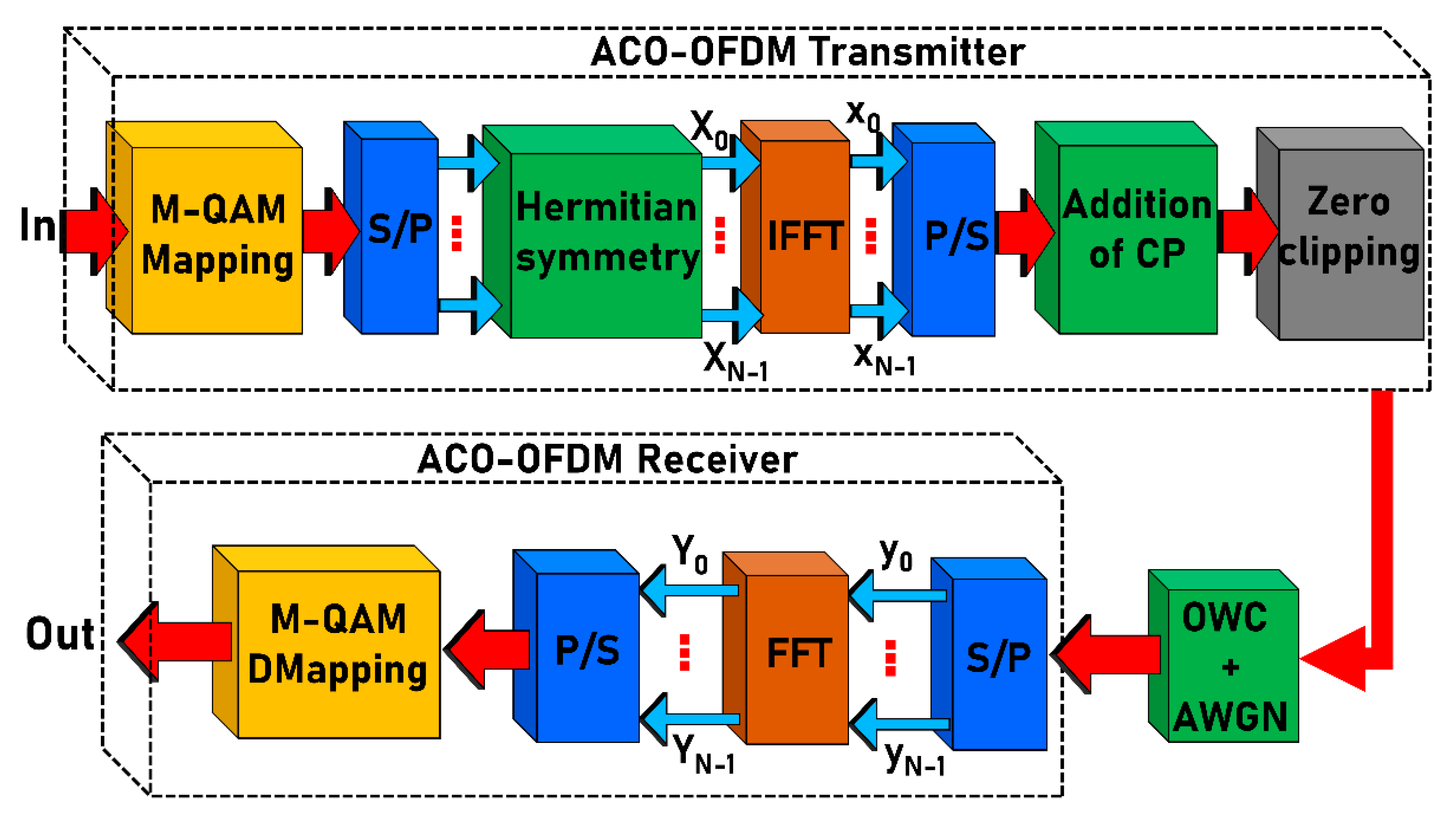
8]. This is a very efficient technique for FSO in terms of transmitted optical power, more so than the methods that use data center (DC) biasing to convert the transmitted data to unipolar. Due to these advantages, we choose to investigate ACO-OFDM in this paper.
In ACO-OFDM, the transmitted signals are made real by transmitting only the odd subcarriers, while the even subcarriers are set to zero [
5,
6,
13]. However, in FSO communication, there is interference that derives from ambient light sources and turbulence. Therefore, estimating the CSI is important in order to successfully recover the data. We will suggest different techniques for estimating the CSI. The authors in [
10] suggest using a least square (LS)-based channel estimator to achieve accurate results in ACO-OFDM FSO systems, while the authors in [
11,
12] suggest using the minimum mean square error (MMSE) and linear MMSE (LMMSE). In the LS estimation method, optimal channel state estimation can be achieved when the channel is optimal, without noise and without interference. The accuracy with MMSE is better and higher than with LS but is limited due to the noise. However, in real environments, such as communication inside data centers, underwater communication, and molecular communication, there is turbulence, which can affect detection of the recovered signals. In the regular estimation methods mentioned above, it is difficult to accurately extract CSI, because in some cases, the turbulence is strong, or the channel is variable and non-deterministic, which makes estimation difficult. Consequently, in these methods, it is necessary to transmit with more power or use other mitigation methods in order to achieve good performance. As a result, there is a need to build ACO-OFDM systems that can enable us to realize a complete communication system without having to know the parameters of the channel model in order to maximize the performance of the communication system. We demonstrate that the use of deep learning (DL) algorithms for recovering the transmitted data in ACO-OFDM modulated signals can be an effective solution for FSO through turbulent channels, thereby improving the performance of the communication system.
Deep neural networks (DNNs) is one of the important algorithms that is widely used in DL. DNNs have tools that enable learning complicated models, which helps to optimize the performance of the entire system by learning relationships between input and output variables through training processes. In recent years, researchers have used DL models in different areas, such as image and speech recognition [
14,
15], and wireless communication systems for encoding, decoding, channel estimation, and signal identification [
16,
17,
18]. The use of DL in wireless communication systems can help improve system performance without the need to know the parameters of the channel or the encoder. In regular communication systems, the system is composed of several blocks, and one tries to maximize the performance of each block separately. However, the use of DL in wireless communication systems allows us to view the transmitter or the receiver as a single unit. The performance of the entire block is maximized by minimizing the bit error rate (BER), rather than trying to maximize each block separately as in regular encoders and decoders. This can improve the performance of the entire wireless communication system [
18]. In recent years, researchers have used DL in different optical communication systems. In [
19], researchers succeeded in using DL for reducing computational complexity in optical communication systems. In [
20], the authors use it in detection through atmospheric turbulence for orbital angular momentum in FSO communication. The authors in [
21] successfully used DL to mitigate fiber-induced nonlinearity. In [
22], DL was used as a solution for the imperfect CSI problem in FSO communication systems. Recently, in [
23], we used DL for improving the performance of on–off keying (OOK) modulation over different FSO turbulence channels.
In this study, we show a new detection method of modulated ACO-OFDM signals using different models of DL. The noisy modulated transmitted data are recovered without the need to know any parameters about either the channel or the encoder. We examined the performance of the DL-assisted ACO-OFDM by generating random data bits modulated by ACO-OFDM. The data were transmitted via a different turbulent channel with additive white Gaussian noise (AWGN). The receiver receives the modulated data with noise and needs to recover the original data bits from the received data using different algorithms of DL, without the need to know anything about the modulation parameters or the parameters of the channel. The developed DL models were compared with one another and also with the regular ACO-OFDM decoder that uses the MMSE estimator, in terms of BER and computational and memory complexity that can affect the power consumption of the system. An improvement in the performance of ACO-OFDM, quantified by a decrease in the BER in all the DL models, was observed, especially over channels with strong or variable turbulence. Our proposed DL models obtain performance that is slightly better than that of an MMSE estimator, especially when the channel is stationary with weak or strong turbulence. In addition, when the turbulent channel is non-stationary and variable, we find a significant improvement in system performance, and the BER is decreased by more than 8 dB compared with regular ACO-OFDM using the MMSE estimator. In addition, our DL decoders run faster than the regular ACO-OFDM decoder, which leads to a significant reduction in the energy consumption of the FSO system.
The rest of this paper is built in the following manner.
Section 2 describes the FSO turbulent channel characteristics and the ACO-OFDM encoder–decoder system. The DL decoders we developed are presented in
Section 3. In
Section 4, we summarize the results of our simulations.
Section 5 presents the conclusions of the study and future perspectives of the work.
3. Our Proposed DL Detection Models
DL is a neuron system model that maps input to output data through a graph that contains several layers. The input data are data with noise after passing through a specific system. The output of the DL system is the original data that the DL wants to detect. Each layer maps the data through nodes, where the first layer is the input data. Each layer depends on the value of the nodes in the previous layer after passing an activation function. DL tries to optimize the performance of the system through two stages. The first is called the training process, and the second is called the prediction process. At the beginning of the training process, the DL system model sets random values to the weights, which are the connections between the nodes in each of two consecutive neighboring layers, and then it changes the weights of the DL model by a gradient descent method in a number of iterations until it reaches the minimum loss between the output of the DL system and the original output. Then, after the training process, the system saves the final weights with the minimum loss and then starts an online process called the prediction process. In this process, the system receives online data and detects the original data, depending on the weights that were saved in the previous process. In recent years, many researchers have used DL for improving the performance of a system in many fields, including speech recognition, wireless communication, optical wireless communication, etc. In [
23], we successfully used DL for improving the performance of OOK modulation over different FSO turbulent channels. The received data are a corrupted version of the data after passing through turbulence, and the output data are the original data bits that we want to detect. Here, we want to use the same concept as in [
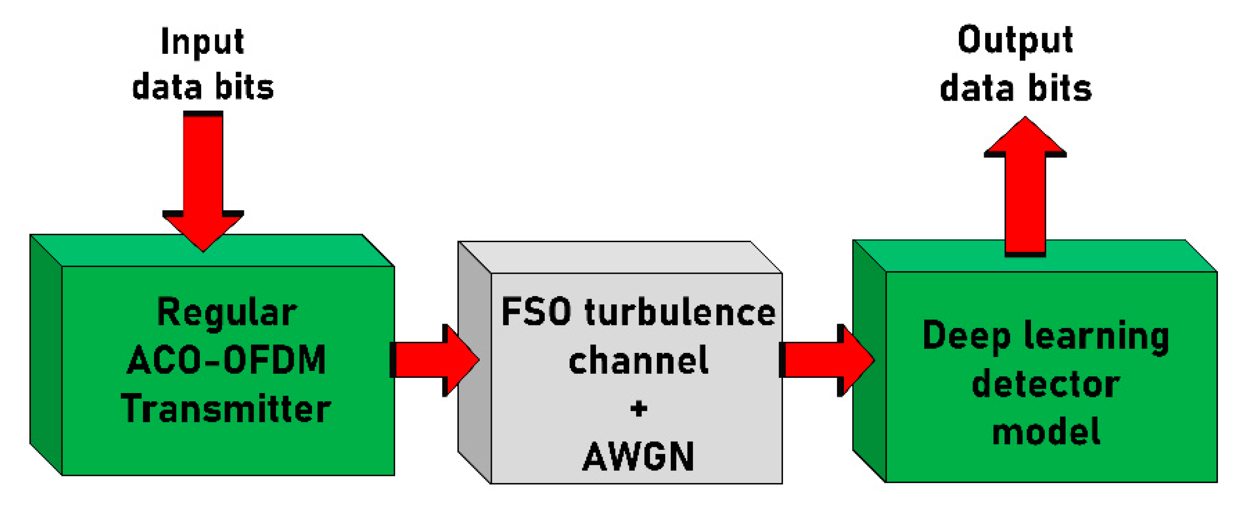
23], to improve the performance of modulated ACO-OFDM signals. We know that this modulation is similar to OOK but is more sophisticated. In both modulation systems, the DL system receives modulated data after it has passed through a turbulent channel with noise and is required to recover the original data bits. In this section, we propose a new DL detection method for ACO-OFDM for FSO communication to enable its use over different turbulent channels and to improve the performance of the FSO communication system when the channel is characterized by strong turbulence or is variable, without the need to know anything about the parameters of the channel. The system of our model is presented in
Figure 2.
In order to use DL systems, we need to learn through a training process, which requires a dataset. For this, we build a dataset by generating random data bits and modulating them by ACO-OFDM modulation, and then, we send them through different atmospheric turbulent channels with AWGN. The receiver recovers the modulated data via a regular ACO-OFDM decoder using an MMSE estimator. For each generated dataset, we create and save two vectors: the input and output vectors. The input vector is the input to the DL system that contains the input data to the ACO-OFDM receiver, which is the modulated data with AWGN after passing through the turbulent channel. The output vector is the original generated data bits. In the training process, the model learns and changes the weights of the DL model until it reaches the minimum loss condition between the output of the DL system and the original output. Then, after the training process, the system saves the final weights with the minimum BER and starts an online process. In the online process, the system can receive any ACO-OFDM modulated data with AWGN after passing through the turbulent channel and detect the original data bits, depending on the weights.
In our work, we used different DL models. In the first model, we used a fully connected (FC) neural network, and in the second model, we used a fully convolutional neural network (FCNN). Schemes of the DL models that we built are presented in
Figure 3 and
Figure 4.
One of the most important things in DL is to properly tune the hyperparameters of the DL network to enable the receiver to recover the original data bits with minimum loss. In general, DL networks should include an input layer, output layer, and several internal layers. We chose the number of nodes in the input layer to be equal to the number of the received data vectors at the receiver that we wanted to demodulate. The number of the nodes in the output layer must be equal to the number of the generated data bits at the transmitter that we wanted to detect. There is no specific way to decide the number of internal layers, so we determined by trial and error until we obtained minimum loss. At the input of our system, we normalized the input data to reduce the variance of the input data scaling. This helped accelerate the training process.
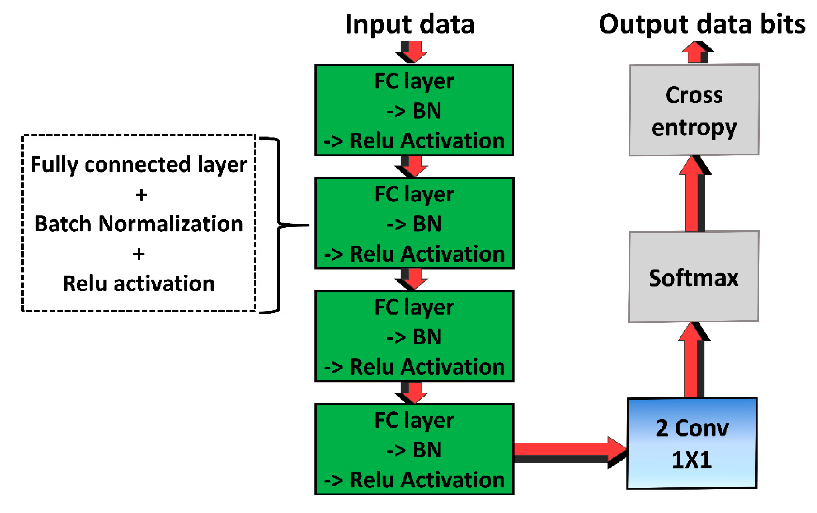
In the first model, we used a FC network with five layers. The first three layers are FC layers with 512 nodes, and the fourth layer is an FC layer with 256 nodes. In the last layer, we used a convolutional layer with two classes with size 1 × 1. Each output node in the last layer detects the recovered bit and decides if it is zero or one, as in
Figure 3.
After each one of the internal layers, which are layers 1 to 4, we use a relu activation function as shown in Equation (12). It is proper for DL in optical communication and is widely used by other researchers:
After the last layer, we use a softmax activation function, given by Equation (13), because softmax activation is an easy function widely used to convert the values of the output data to probabilities between 0 and 1.
Then, we use the cross-entropy loss function in (14), which is suitable for detecting a vector of data by minimizing the distance between the original data and the predicted data, where p is the probability of the original data bits and q is the estimated output probability of our DL system which we require to be minimum through the training process.
The output layer of our model determines the value of each and every bit—if that bit is 0 or 1—by calculating cross entropy loss. This yields a minimum distance loss between the output of the DL system and the original data.
In the second model, we use FCNN. The concept is taken from [
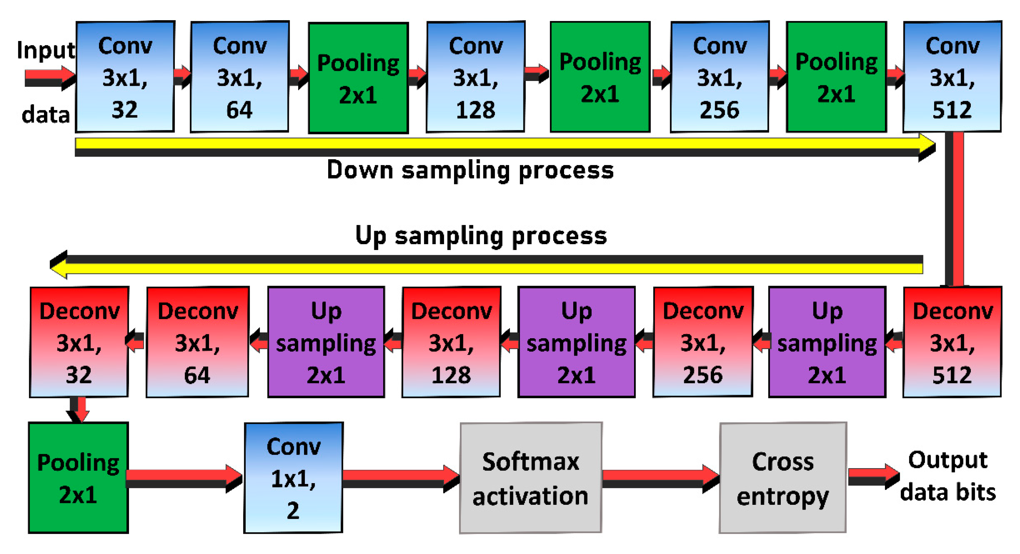
11], where it is proposed for image segmentation, which means determining whether each pixel in the output image is foreground or background. We used FCNN because the aim of our network is to make a semantic segmentation for each output bit. FCNN includes two processes, a down-sampling process and an up-sampling process. The down-sampling process comprises a number of convolutional and pooling layers used to detect high-resolution information in the image. The up-sampling process is the inverse process of the down-sampling process and comprises a number of de convolutional and up-sampling layers, which are used to extract the precise localization of the extracted data after the down-sampling process. The output layer of the system is a convolution layer that contains two channels: one channel predicts if this pixel is background, and the other predicts if it is foreground. In our FCNN model, we used the concept in [
11], but we changed it to be suitable for our problem. Our FCNN model receives input vectors with noise and performs a number of operations on this input vector by two processes, as in the FCNN models: a down-sampling process that comprises a number of convolutional layers with pooling layers in order to interpret the data and then to know the precise localization for the data extracted by the up-sampling process. In the down-sampling process, we used convolutional layers of 32 filters, each of size 3 × 1, and then we used four convolutional layers with filter sizes 64, 128, 256, and 512, each filter of size 3 × 1, between each two layers. We down-sampled the size of the data by pooling. After this process, we used an inverse process of four deconvolutional layers with sizes 512, 256, 128, and 64 filters. Each filter is of size 1 × 3. We up-sampled a 1 × 2 layer between each two deconvolutional layers, as shown in
Figure 4. After each internal layer, we used a relu activation layer, as given above in Equation (12), with batch normalization. After these two processes, we used a pooling layer followed by a convolutional layer of two filters, each one of size 1 × 1. We apply softmax activation as in (13) and use a cross-entropy loss process to obtain the minimum loss between the original data and the output of the DL system as in (14). At the outputs of our systems, we get two values of accuracy and loss. The model trains over a number of iterations until we obtain results with maximum accuracy and minimum loss. The BER is calculated as
, and
is the ratio of number of correct predictions to the total number of input samples. Performances of the DL decoder and the regular ACO-OFDM decoder that used the MMSE estimator are compared. In the next section, we present the results of our proposed DL models and compare them with the results of the ACO-OFDM decoder that uses the MMSE estimator.
4. Simulation Results
In this section, we describe the simulation results of our DL models and compare them with the simulation results of regular ACO-OFDM schemes in terms of performance and energy consumption. Our aim is to replace the regular ACO-OFDM receiver with the DL systems that we built. In order to check our DL models, we needed to generate datasets of input and output data vectors. The input to the DL system is the modulated data received at the input to the receiver. The output of the DL system is the detected data bits. Through the training process, the DL system tries to learn to recover the data in a number of iterations until it succeeds in reaching the minimum distance between the original and the recovered data bits. The dataset of our DL systems includes 10,000 random input–output vectors built by the MATLAB program. We built our DL decoders using Tensorflow software. The output vectors are the output of the DL decoder and are of size 256 data bits of 0 and 1. The input vectors are input ACO-OFDM data bits modulated by 16 subcarriers. We run our simulations on a computer with a CPU Intel Core i7-7500U 2.7 GHz.
We tested our DL models and compared them with the standard ACO-OFDM decoder system for different levels of turbulence in the channels. We passed our modulated ACO-OFDM data through weak and strong turbulence in cases of slow fading with a stationary channel and fast fading with a non-stationary channel. The strength parameters for the different turbulence channels that we used and the hyperparameters of our DL systems are presented in
Table 1.
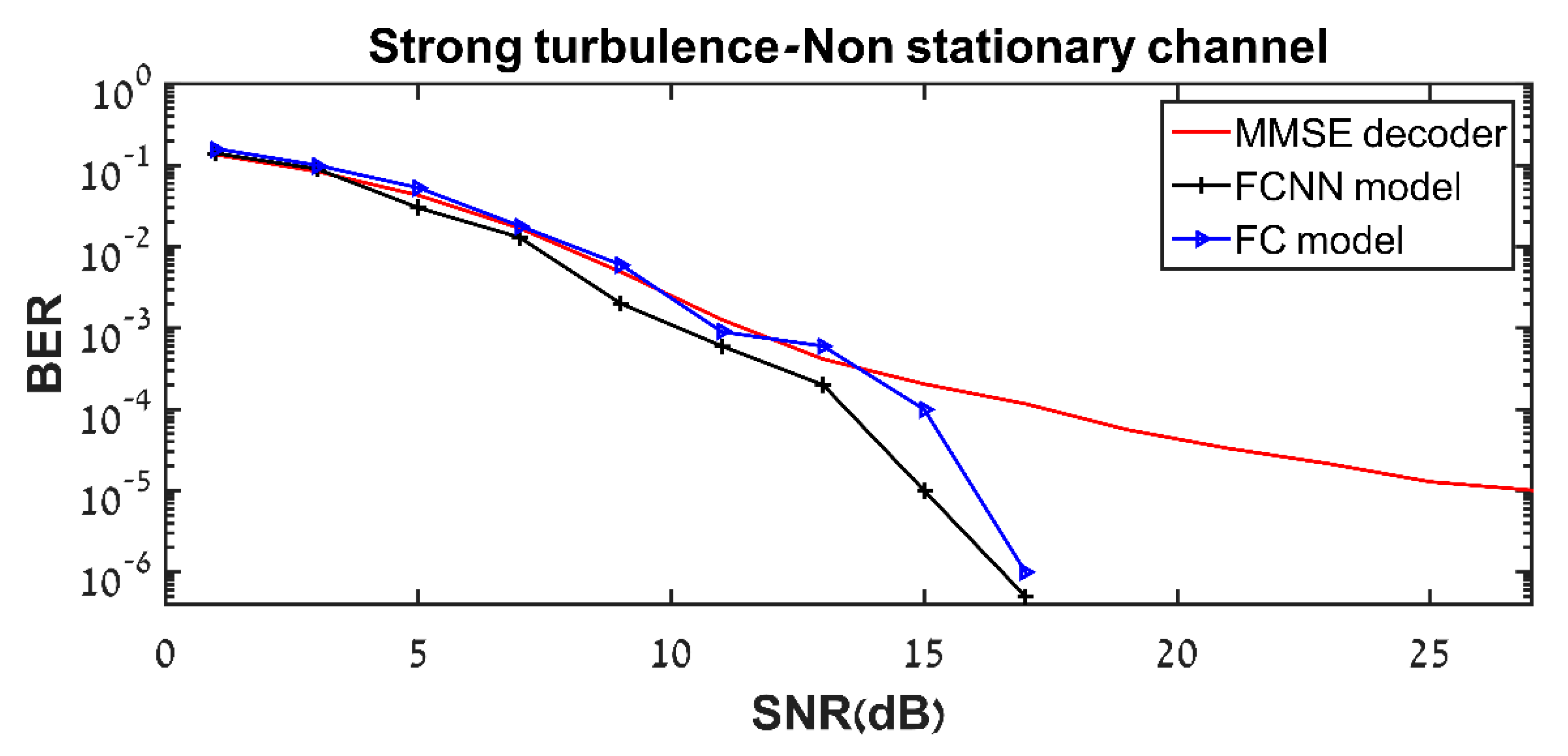
The BER performance results of our DL models compared with the regular ACO-OFDM decoder system when the channel is with fast fading and non-stationary are presented in
Figure 5 for strong turbulence.
The red curve is the BER performance of the ACO-OFDM decoder using the MMSE estimator, the black curve is the results of our FCNN model, and the blue curve is the results of our FC DL model. We see that the results of our DL models are very close to each other and very close to results of the regular ACO-OFDM until SNR = 13. After this, our DL models improve the performance of the ACO-OFDM system and lead to a significant decrease in BER compared to the regular ACO-OFDM decoder. For example, after SNR = 14, the BER performance of our models decreases rapidly to values less than 10−6. On the other hand, the BER performance in regular ACO-OFDM for the same SNR is equal to 10−4, and at SNR = 25, it reaches 5.10−4 and does not decrease further, because the channel is non-stationary, and it is difficult for the MMSE estimator to estimate the CSI in order to get optimal performance.
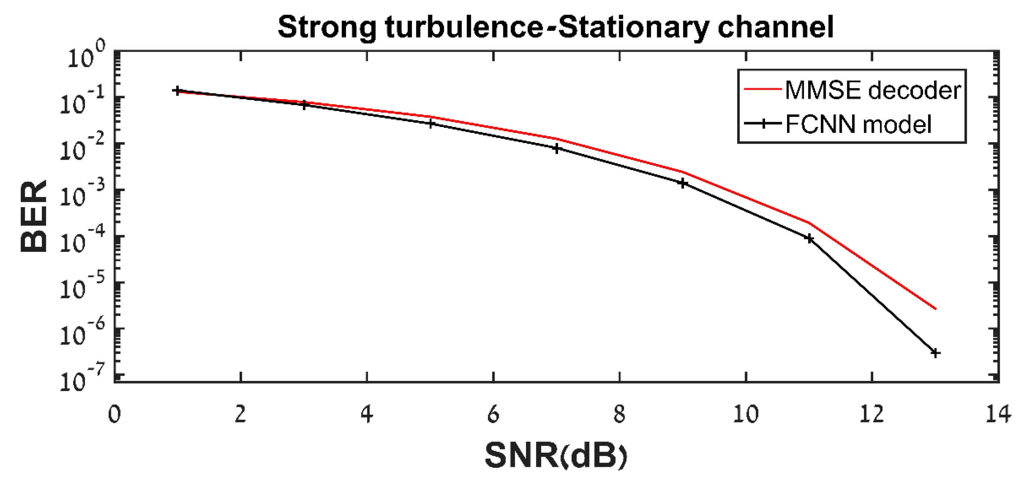
The results of our FCNN DL model when the channel is stationary with slow fading and strong turbulence are presented in
Figure 6.
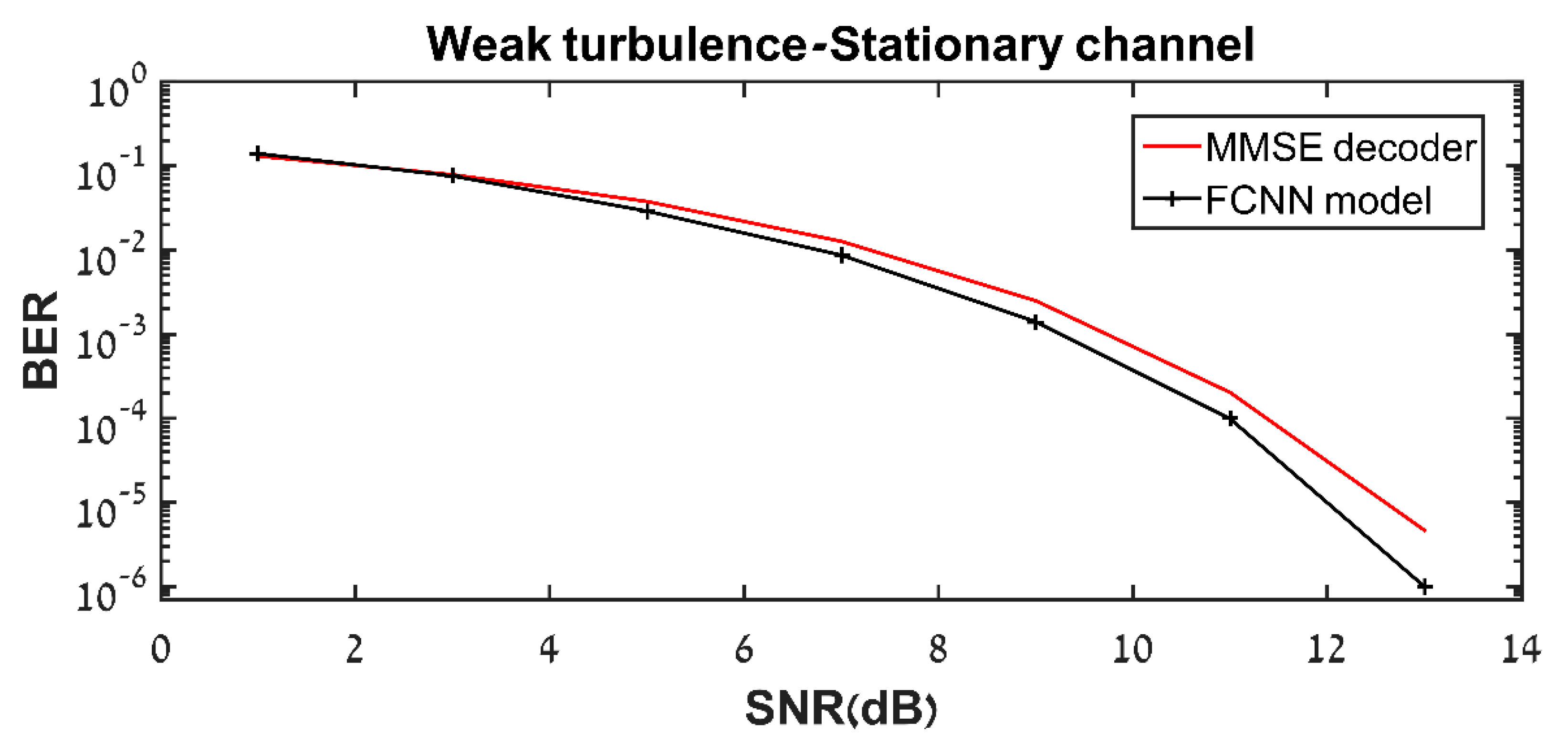
The results of our FCNN DL model when the channel is stationary with weak turbulence are shown in
Figure 7.
In
Figure 6 and
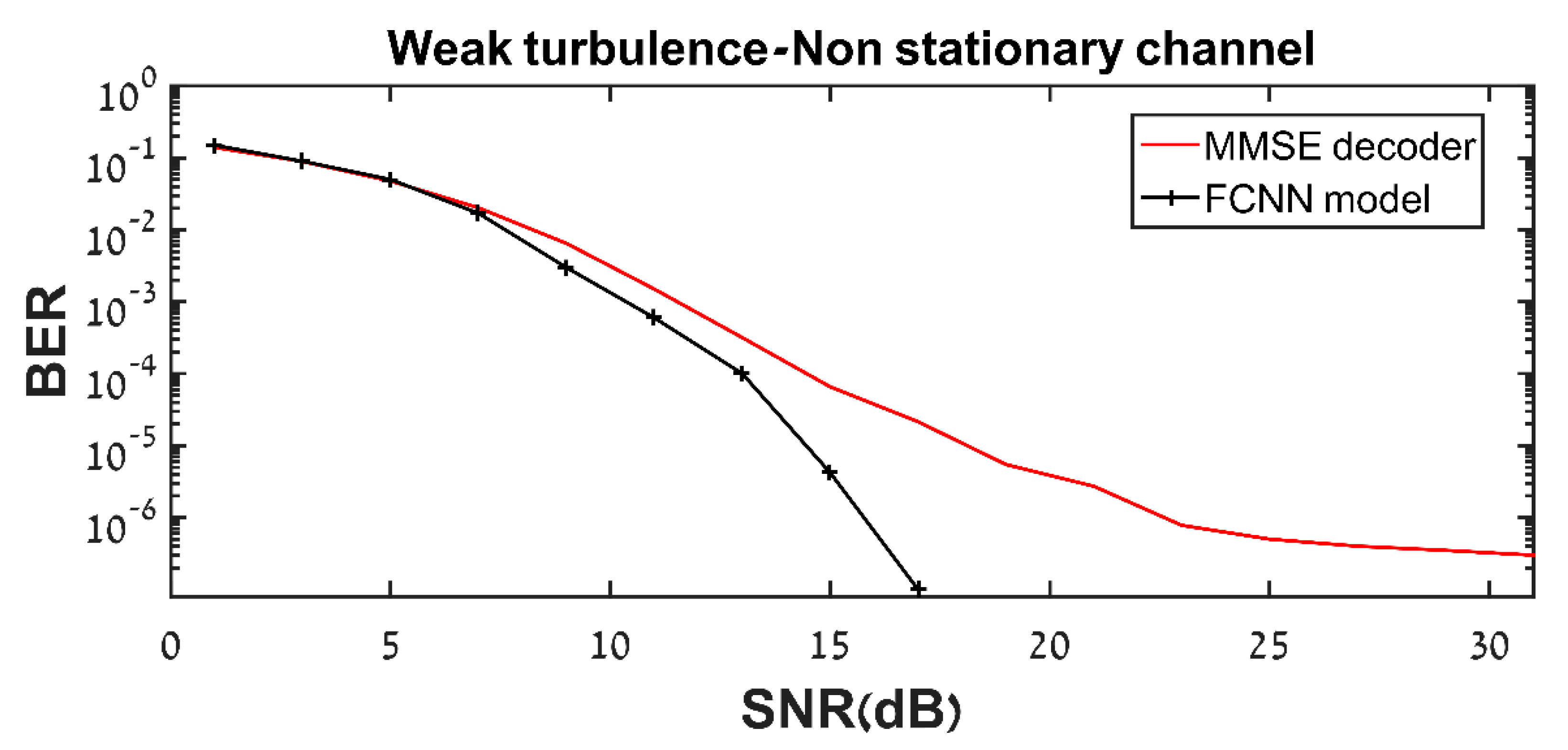
Figure 7, the red curve represents the BER performance of the regular ACO-OFDM decoder using the MMSE estimator, and the black curve represents the results of our FCNN model. We see that our FCNN DL model yields performance very close to that of the MMSE estimator when the channel is stationary with weak turbulence or with strong turbulence. However, the advantages of our DL models are clearly shown in
Figure 8. When the channel is characterized by weak turbulence and is non-stationary with fast fading, the regular ACO-OFDM decoder using the MMSE estimator does not succeed in recovering the corrupted data. Since for the same BER this method requires higher SNR, it consumes much more energy compared to our DL models, which succeed in recovering the data with less energy consumption and manage to decrease BER by more than 8 dB. For example, when the SNR is larger than 25, the regular ACO-OFDM decoder yields a BER performance equal to 10
−6 and does not achieve a lower value than this, even at higher SNR. However, in our FCNN DL model, when the SNR is 17 dB, we succeed in getting BER performance equal to 10
−7, and with this SNR, we recover the transmitted data without errors. In other words, we get a BER equal to zero.
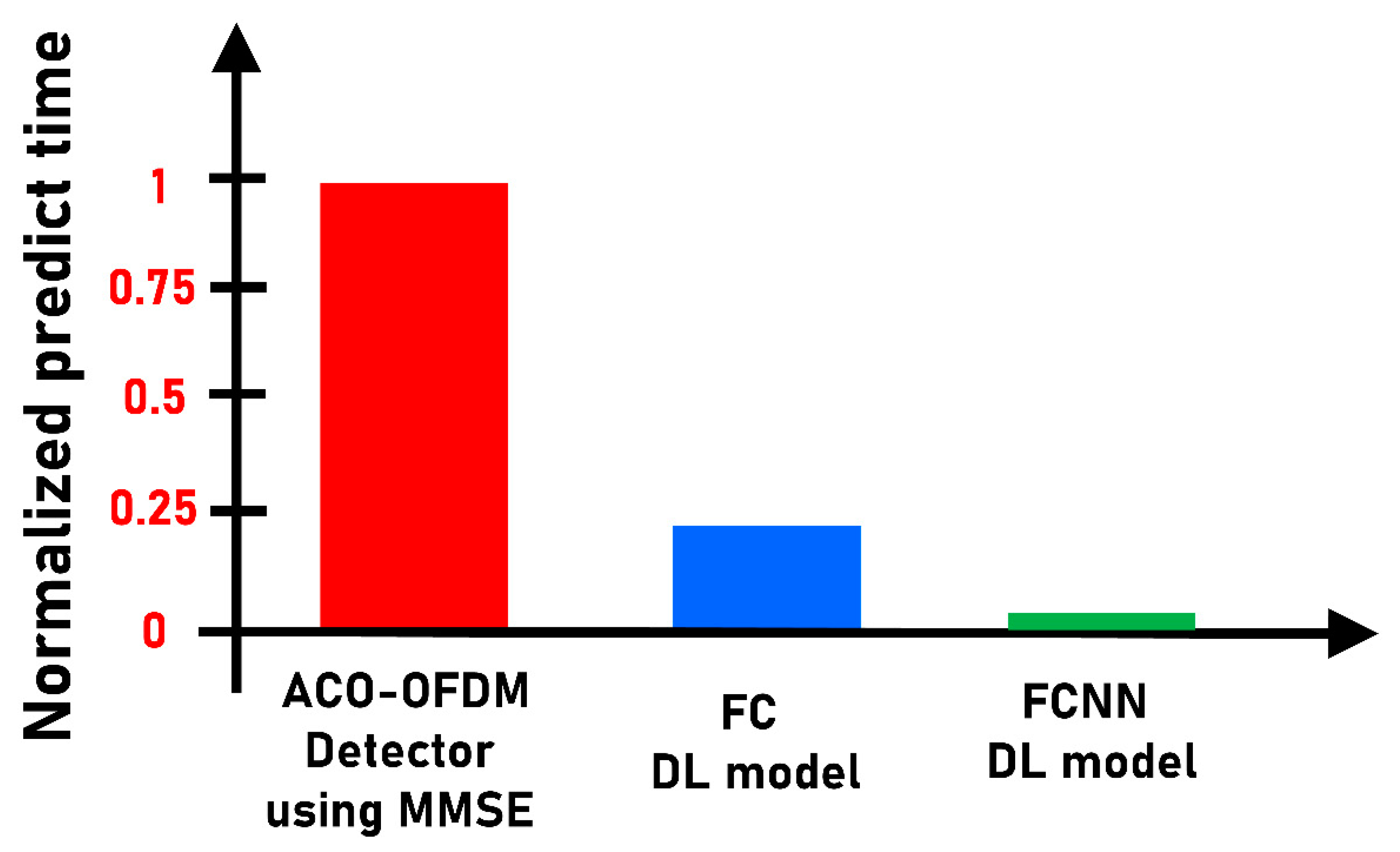
In addition to this, another advantage of our DL models is that they are faster than the regular ACO-OFDM decoder. The prediction time of our DL models after the training process is faster than that of the regular ACO-OFDM decoder, as shown in
Figure 9.
Our FCNN DL model recovers the data more than 10 times faster than the regular decoder. In addition, the prediction time is three times faster than for our FC DL model. This is because the nodes in each layer in the FC model are connected to all the nodes in the next layer. This take time, but the nodes in each layer in the FCNN model are not connected to all the nodes in the next layer. The DL method consumes less time and less energy than the FC model and the regular ACO-OFDM detector. After the training process, we do not need, as in the regular ACO-OFDM decoder, to go through all the blocks of the decoder one by one, which would consume time and energy. After the training process, the weights are saved in the system, and any online received modulated ACO-OFDM can be recovered directly.
Therefore, in this work, our DL models succeed in recovering the received ACO-OFDM data when the channel is with strong and weak turbulence, when the channel is stationary with slow fading, and when the channel is non-stationary with fast fading. Our DL models offer performance very close to that of ACO-OFDM using the MMSE estimator, and it is even slightly better when the channel is stationary. However, when the channel is fast fading and non-deterministic, our DL models can recover the data with better performance than the MMSE estimator. When the channel is variable, this estimator does not manage to reach optimal performance because the channel is not stationary. In addition to these advantages, our models work faster than the regular ACO-OFDM decoder, so they are very efficient for use in real environments where energy saving is important.


