Design and Analysis of a Novel Flexure-Based XY Micropositioning Stage

Abstract

Flexure-based micropositioning stages with high positioning precision are really attractive. This paper reports the design and analysis processes of a two-degree-of-freedom (2-DOF) flexure-based XY micropositioning stage driven by piezoelectric actuators to improve the positioning accuracy and motion performance. First, the structure of the stage was proposed, which was based on rectangular flexure hinges and piezoelectric actuators (PZT) that were arranged symmetrically to realize XY motion. Then, analytical models describing the output stiffness in the XY directions of the stage were established using the compliance matrix method. The finite element analysis method (FEA) was used to validate the analytical models and analyze the static characteristics and the natural frequency of the stage simultaneously. Furthermore, a prototype of the micropositioning stage was fabricated for the performance tests. The output response performance of the stage without an end load was tested using different input signals. The results indicated that the stage had a single direction amplification capability, low hysteresis, and a wide positioning space. The conclusion was that the proposed stage possessed an ideal positioning property and could be well applied to the positioning system.

1. Introduction

Micro/nanopositioning technology is essential for various applications in many research and technical fields, such as microelectromechanical systems (MEMS), ultra-precision machining and measurement, micro-assembly, biological processes, manipulation, and other applications [1,2,3,4,5,6,7,8]. For a scanning system, a parallel kinematic piezoelectric actuator (PZT) XYZ scanner was proposed, which could achieve high bandwidth and low coupling errors [9]. A new two-degree-of-freedom compliant parallel micromanipulator (CPM) utilizing flexure joints was proposed for two-dimensional nanomanipulation [10]. The XYZ micromanipulator has applications that include moving and positioning microcomponents, such as mirrors, lenses, and gratings. It can position microcomponents in the X-, Y-, and Z-directions by using three independent linear inputs and has achieved out-of-plane displacements [11]. In consideration of the wide application demands in many areas, micropositioning stages are the core equipment for realizing micropositioning. In recent decades, it has achieved rapid development and plays an important role in today’s engineering applications. For example, the parallel kinematic XY flexure mechanism was designed based on systematic constraint patterns for realizing large ranges of motion without causing over-constraint or significant error motions [12]. A novel flexure-based mechanism with three degrees of freedom driven by three piezoelectric actuators focused on achieving kinematics with X-direction motions decoupled from those in the Y- and θ-directions [13]. The piezo-actuated XY stage with integrated a parallel, decoupled, and stacked kinematics structure was used for micro/nanopositioning applications and a novel flexure-based XY micropositioning stage driven by electromagnetic actuators with high moving range and resolution was also produced [14,15]. Based on the above analysis, numerous positioning stages applied in various fields with various types and functions have received wide attention and can be found in recent research [16,17,18,19,20,21,22,23,24,25,26].

In particular, two-degree-of-freedom (2-DOF) micropositioning stages meet most requirements of practical applications. A micropositioning stage based on flexure hinges can provide an output displacement with desirable properties for realizing micro/nanometer resolutions. Compared with conventional linkage mechanisms, flexure hinges possess inherent advantages, such as no friction, no backlash, repeatable motion, no need for lubrication, and a low cost [27,28,29]. Flexure hinges are utilized as elastically deformable rotation/translation joints for precision motion in micropositioning stages. It is important to achieve both a high natural frequency and motion accuracy. So far, there have been a large number of studies that have explored the performance of various flexure hinges with different structures [30,31,32,33,34,35,36], such as the leaf-spring hinge, cross-axis flexural pivots, and cartwheel hinges. Different flexure hinges have their own characteristics. The various flexure hinges are most often used in the positioning stage as a guide mechanism to make them ideal for wide use in scientific instruments. In the proposed structure of the stage, to simplify the design, the rectangular beam with different geometric parameters was combined to form different flexure hinges to reduce the complexity due to the excessive number of structural parameters. Meanwhile, utilizing multiple instances of the same parallel flexure hinge instead of a single hinge to connect two rigid links can enhance the performance of the stage [37].

Except for the factors in terms of the stage structure, actuators and materials, fabrication accuracy, and assembly errors, sensors and unknown disturbances will likely reduce the positioning precision of the micropositioning stage [38]. According to its different working conditions, the driving mode is generally divided into three types: direct drive actuators, inertial drive type actuators, and worm drive type actuators. In contrast with the conventional motors, piezoelectric actuators have lots of superiorities, such as no electromagnetic radiation, compact structure, self-lock at power-off state, short response time, and high precision [39,40,41]. Herein, the direct-drive piezoelectric actuator [42] has been chosen to obtain high resolutions and stability, while it is likely to limit the stage stroke [43]. The stage includes wire cutting processing and open-loop control to achieve motion performance.

Based on the aforementioned analysis, to improve the performance in terms of the accuracy and motion of the positioning stage, a novel differential drove two-dimensional positioning stage was designed and analyzed in this paper. The organization of the paper is as follows. Section 2 briefly describes the structure of the positioning stage, where the core part and the form of the drives are introduced. Section 3 describes an analytical model of the proposed stage based on the compliance matrix method. Finite element analysis was used to validate the performance of the proposed 2-DOF flexure-based XY micropositioning stage, where the results are presented in Section 4. The experiments are discussed in Section 5 before the conclusions are given in Section 6.

2. Mechanical Design

The proposed 2-DOF flexure-based XY micropositioning stage is shown in Figure 1 (the scale for the geometrical dimensions is 1:30 (mm)). The overall structure of the stage is symmetrical along the Y-axis. Two piezoelectric actuators located at the frame are respectively mounted along the X-axis (piezoelectric actuator-1 (PZT-1) and piezoelectric actuator-2 (PZT-2) in Figure 1). The contact condition between the piezoelectric actuator and the driving point was assumed to be Hertzian contact. The actuators are preloaded by a thread and in contact with flexure hinges through the ball-screw (part G in Figure 1). The power amplifier controlled by a personal computer (PC) is used to supply control voltage signals for the expansion and retraction of the piezoelectric actuator. The core part of the positioning stage that consists of an output stage (part D in Figure 1) and chains (X- and Y-axes), as shown in Figure 1.

In the stage, the flexure hinge of the chains is a rectangular beam hinge with different scale parameters. Compared with other types of flexure hinges, a rectangular flexure hinge (Figure 2a) has more advantages, such as ease of processing and a larger motion displacement. In the X-axis chain, the double parallel rectangular (Figure 2b) beam was chosen as the guide link between the input and the output stage (part D in Figure 1). Parts A and E are symmetrical along the Y-axis to avoid the parasitic movement in the vertical direction and greatly increase the motion stability. In the Y-axis chain, the part B and F links are the structure composed of a single rectangular beam (Figure 2c), while it reduces the structural static stiffness to obtain a larger motion displacement.

The displacement input from the piezoelectric actuators is transferred by displacement transmission units (part C in Figure 1). Two units are arranged in parallel (Figure 3a) such that it greatly increases the stage stiffness and makes motion transmission more stable. The structure of the displacement transmission unit is shown in Figure 3b. In the simplified schematic (Figure 3c), the input displacement is transferred separately to the X- and Y-axes, while their values are dependent on the angle α. The value of different angles brings different transmission effects. This issue is not discussed in detail herein. The appropriate value was chosen based on actual experiences, discussed in Section 3, for analyzing the proposed 2-DOF flexure-based micropositioning stage.

The two aforementioned piezoelectric actuators were arranged symmetrically along the X-axis to realize the differential drive for the stage. Herein, (1) if two actuators are given the same input displacement, the output stage achieves excellent single-axis positioning performance along the Y-axis; (2) if given different displacements, the output stage achieves X-axis and Y-axis displacements to realize 2-DOF positioning. The positioning range depends on the difference value between the input displacements of PZT-1 and PZT-2 (Figure 1). The workspace is an arc, as shown in Figure 4. (1) When only one PZT (PZT-1 or PZT-2) is working, the motion trajectory of the stage is the outer contour of the working space. The point b or d, which are reached depending on the chosen PZT actuator, are at the limits of the travel range. (2) When the two PZT actuators are not working, point a in Figure 4 is the initial point of the working space. (3) When the input of the two PZT actuators is the same, the center of the stage is on the line ae. Point c is half the travel range of the two chosen PZT actuators. Point e is at the limit of the travel range of the two chosen PZT drivers. The working space of the stage depends on the stroke of the chosen PZT actuators’ travel range. When only one PZT is working, the inactive one acts as the blocking barrier and decreases the positive x-axis. However, the displacement in the X-axis direction is produced by two piezoelectric actuators. The actual maximum motion length in the X-axis direction is twice the maximum displacement of a single chosen PZT actuators.

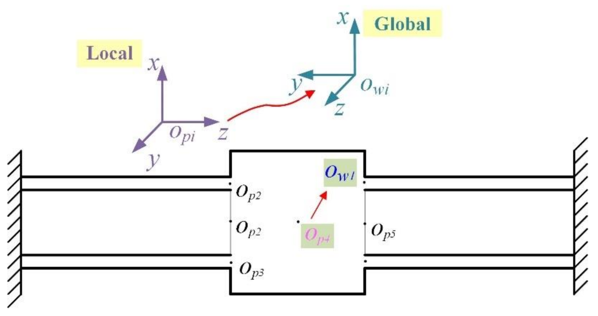
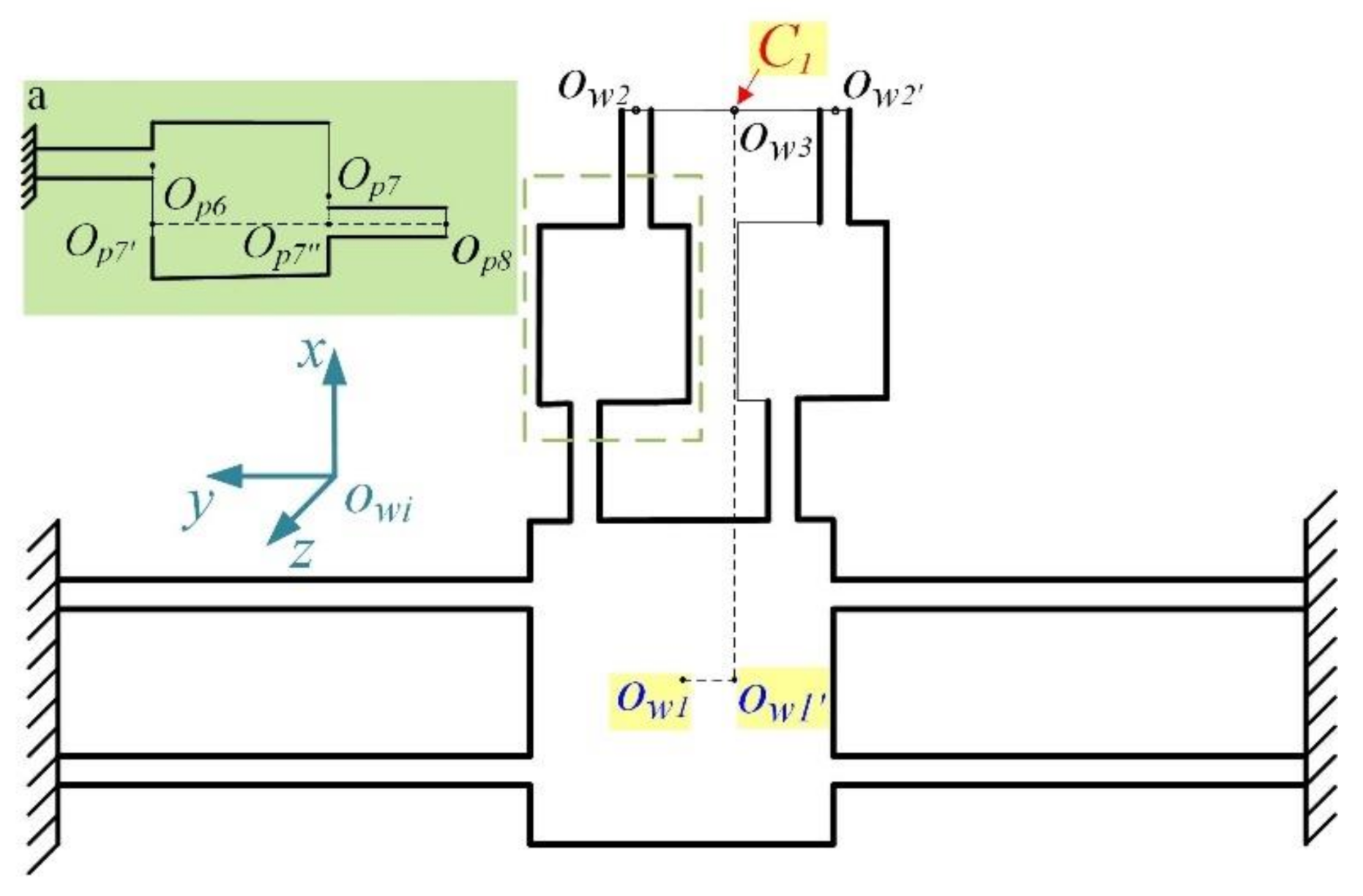
3. Mathematical Model

The compliance matrix method was used to calculate the mathematical model. First, the compliance matrix of a single flexure hinge was calculated. Second, the compliance model of the core part was calculated. Finally, the compliance model of the whole structure was obtained. The detailed formula derivation process of the compliance matrix of the rectangular beam hinges [34], the rotation matrix, and the translation matrix are given in Appendix A and Appendix B. If $C_{p_i}$ represents the compliance matrix of the flexure hinge in the local coordinate system, $C_{w_i}$ represents its compliance matrix in the global coordinate system. The conversion relationship between the local and global compliance matrices is:

$$C_{w_i}=R_{i}P\left(r_i\right)C_{p_i}P{\left(r_i\right)}^T{R}_i{}^T,$$

(1)

where $R_i$ is the local-to-global rotation matrix and $P\left(r_i\right)$ is the local-to-global translation matrix.

While having m flexure hinges in series, the compliance matrix of m flexure hinges is:

$$C_{p-m}={\displaystyle \sum }_{i=1}^m{C}_{p_i}.$$

(2)

When having n flexure hinges in parallel, the compliance matrix of n flexure hinges is:

$$C_{p-n}={\left[{\displaystyle \sum }_{i=1}^n{\left(C_{p_i}\right)}^{-1}\right]}^{-1}.$$

(3)

The general mathematical model from (1)–(3) and the equations in Appendix A and Appendix B (Equations (A1), (B1)–(B3)) are applied here as the mathematical model of the core part and the whole structure. As shown in Figure 5, the local coordinate $O_{Pi}$ refers to the core part and the global coordinate $O_{wi}$ refers to the whole structure. The local compliance matrix of this part to the point $o_{p4}$ by rotation and translation from points $o_{p1}$,$o_{p2}$,$o_{p3}$, and $o_{p5}$ in Figure 5 is given as:

$$C_{o_{p4}}={\left[{\left(C_{o_{p2-4}}\right)}^{-1}+{\left(C_{o_{p5-4}}\right)}^{-1}\right]}^{-1}.$$

(4)

Conversion to the global coordinates in Figure 5 is given as:

$$C_{o_{w1}}=R_x\left(\frac{\pi }{2}\right)C_{o_{p4}}{R}_x{\left(\frac{\pi }{2}\right)}^T,$$

(5)

where the detailed process is in Appendix C (A5)–(A12).

As shown in Figure 6, the point $o_{p8}$ in displacement transmission units is given as:

$$C_{o_{p8}}=C_{o_{p6-8}}+C_{o_{p7-8}}+C_{o_{p6}}.$$

(6)

The transformation using matrix $O_{o_{p8}}$, which converts to the global coordinates, is given as:

$$C_{o_{w2}}=R_x\left(\frac{\pi }{2}\right)R_z\left(\frac{\pi }{2}\right)C_{o_{p7}}{R}_z{\left(\frac{\pi }{2}\right)}^T{R}_x{\left(\frac{\pi }{2}\right)}^T.$$

(7)

$C_1$ is the point $o_{p4}$ reached using rotation and translation from points $o_{w1}$, $o_{w2}$, and $o_{w3}$ in Figure 6 as follows:

$$C_1={\left[{\left(C_{o_{w2-3}}\right)}^{-1}+{\left(C_{o_{w{2}^{\prime }-3}}\right)}^{-1}\right]}^{-1}+C_{o_{w1-3}},$$

(8)

where the detailed process is in Appendix C (A13)–(A20).

The point $o_{p10}$ in displacement transmission units is given as:

$$C_{o_{p10}}={\left[{\left(C_{o_{p9-10}}\right)}^{-1}+{\left(C_{o_{p11-10}}\right)}^{-1}\right]}^{-1}+C_{o_{p12-10}}.$$

(9)

$O_{o_{p10}}$ converts to the global coordinates in Figure 7 as follows:

$$C_2=C_{o_{w4}}=R_z\left(\frac{\pi }{2}\right)R_x\left(\frac{\pi }{2}\right)C_{o_{p10}}{R}_x{\left(\frac{\pi }{2}\right)}^T{R}_z{\left(\frac{\pi }{2}\right)}^T,$$

(10)

where the detailed process is in Appendix C (A21)–(A25).

In Figure 8, $C_{w_1}$, $C_{w_2}$, $C_{w_3}$, and $C_{w_4}$ converts to the core of the output stage via rotation and translation to obtain $C_w$. The compliance matrix of the whole structure is given as

$$C_w={\left[{\left(C_{w_1}\right)}^{-1}+{\left(C_{w_2}\right)}^{-1}+{\left(C_{w_3}\right)}^{-1}+{\left(C_{w_4}\right)}^{-1}\right]}^{-1},$$

(11)

where the detailed process is in Appendix C (A26)–(A29).

As such, the compliance matrix of the whole structure $C_w$ was obtained. The detailed formula derivation process is given in Appendix C. The structural parameters of the stage designed in the experiments are shown in

Table 1. Precision positioning stage structural parameters.

Part	Symbol	Length (mm)
Part 1	$a_1$	0.7
	$b_1$	10
	$l_1$	15
Part 2	$a_2$	0.7
	$l_2$	3
Part 3	$a_3$	0.7
	$l_3$	8
Part 4	$a_4$	6
	$l_4$	8
Part 5	$a_5$	0.7
	$l_5$	15

and Figure 9. $a_i$,$l_i$, and $b_i$ represent the lengths of x-, y-, and z-axes, respectively. In the z-axis, all lengths were the same ($b_1=b_2=b_3=b_4=b_5$). These parameters in Table 1 were brought into the equations. MATLAB (MathWorks, Inc., version 2018) was used to calculate the compliance matrix. $C_w$ is given as Equation (12). Its unit is micrometers per newton. Meanwhile, the equation between the input force and output displacement was obtained using Equation (13), according to the relationship between force and displacement ($X=CF$). The output stiffness in the x- and y-directions were 1.34 μm/N and 0.438 μm/N. The theoretical equations is shown to be verified through the numerical simulation in Section 4.

$$C_w=\mathrm{diag}\left(1.3,0.438,0.00415,1.6\times {10}^{-4},1.9\times {10}^{-4},5\times {10}^{-4}\right)$$

(12)

$${\left[{\delta }_x, {\delta }_y\right]}^T=\left[1.3f_x, 0.438f_y\right]$$

(13)

where ${\delta }_x$ and ${\delta }_y$ respectively represent the displacement components in the x- and y-directions.

4. Numerical Simulations

The finite element analysis of the stage was carried out using ABAQUS (Dassault Systemes, version 2017). Considering the simulation’s computational efficiency, the simulation model was simplified by only including all motion links and the output stage. The virtual prototype was created using SOLIDWORKS (Dassault Systemes, version 2018), as shown in Figure 10a. The analysis process was divided into two steps: (1) static analysis and (2) modal analysis.

Regarding the simulation, the material parameters are shown in

Table 2. Material parameters used in the simulation.

Material	Density ρ (kg/m3)	Young’s Modulus E (GPa)	Poisson Ratio ν	Shear Modulus G (GPa)
Aluminum	2.7 × 103	70	0.36	25.6

. The ends of all the links were fixed. Loads were applied at the surface in the x-axis. First, given an input force of 60 N in a single direction (simulating only one PZT working), the output stage displacement was extracted. The displacements in the X- and Y-directions are shown in Figure 11a,b, respectively. The simulation analysis results are shown in

Table 3. Comparison between the theory and simulation output displacements.

Axis	Theory (μm)	Simulation (μm)	Error (%)
$x$	78	76.3	2.2
$y$	26.3	24.9	5.3

. The displacements in the X- and Y-directions were 76.3 μm and 24.9 μm, respectively. According to Equation (13), the theoretical values were 78 μm and 26.3 μm, respectively. The error between the theoretical calculation and the simulation analysis was within 5.3%. The displacement ratio between the X- and Y-directions were 3.06 (simulation) and 2.96 (theoretical). The X-direction stiffness was approximately 3 times that of the Y-direction. The simulation results verified the reliability of the theory. The stress figure of the proposed stage under the input limit state of the piezoelectric actuator is shown in Appendix D, (Figure A9, Figure A10, Figure A11 and Figure A12).

The frequency results for the stage are shown in Figure 12 and

Table 4. Natural frequencies.

Modal Analysis	First	Second	Third	Fourth	Fifth
Frequency (Hz)	1088.9	2240.1	5989.9	7866.9	10,739

. The first to third natural frequencies were 1088.9 Hz, 2240.1 Hz, and 5989.9 Hz, respectively. The third natural frequency was much larger than the first and second, which illustrates that the vibration had little effect on working conditions.

Considering the characteristics of the selected piezo-actuator for verifying the performance of the structure, the range of input displacements was assumed to be 0–20 μm in the simulations. The performance was assessed in terms of the corresponding output displacements. (1) Given a single-direction displacement input, the output displacement of the output stage was extracted to get the displacement relationship as shown in Figure 13 and Figure 14. In the X-axis direction, the ratio was close to 1 between the input and output, and the average error was 3.83%. The material was considered linear elastic in the simulation. The result showed that there was also a slight displacement in the Y-axis, as shown in Figure 14. Regarding the X-axis direction, the displacement ratio of the X- to Y-axes was 10.07%. (2) Given a double-direction displacement input, if the input value of the two piezoelectric actuators was the same, the output stage motion was only in the Y-axis direction. As shown in Figure 15, the ratio was 2.77 between the input and output. The coupling error was 1 × 10⁻⁵%. In the case of using this input method, the positioning stage had a better displacement amplification capability in a single direction, which increased the positioning range. This performance of the stage expands the scope of application. It can not only be used as an independent positioning stage but can also be used as a unidirectional amplifier module with the application of multiple units in combination (two piezoelectric actuators are driven together to realize Y-axis motion).

5. Experiments

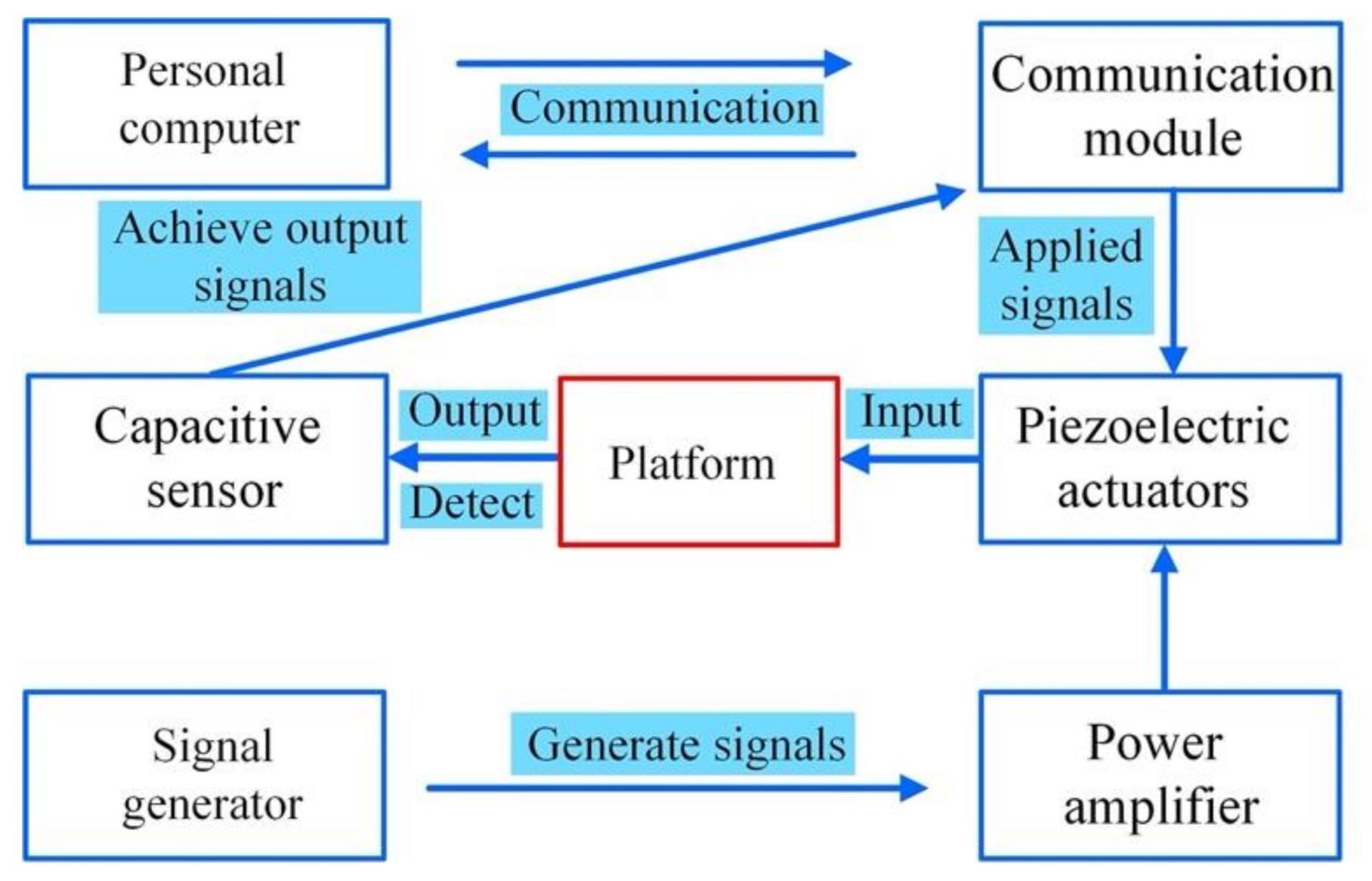
5.1. Method

The experimental test method to evaluate the stage is shown in Figure 16. The software in the PC provided the interface for the user. The signal was generated by a signal generator. The input was amplified by a power amplifier and applied to the piezoelectric actuators of the positioning stage. The displacements of the output stage were measured using capacitance sensors. A capacitance detection module was used to achieve the output signal acquisition in each direction. Using the developed experiment test system, a series of experiments were conducted to further verify the performance of the stage.

The test system shown in Figure 17 consisted of a personal computer (PC), signal generator (voltage range: 0.5–2 V, frequency range: 0–1000 Hz, Siglent model: Sdg805, Shanghai, China), two piezoelectric actuators (Physik Instrumente (PI), PI-842.6, Karlsruhe, Germany, where the parameters are shown in

Table 5. The parameters of the PZT (PI-842.60).

Parameters	P-842.60	Unit	Tolerance
Travel range at 0 to 100 V	90	μm	±20%
Resolution	0.9	nm
Static large-signal stiffness	10	N/μm	±20%
Push force capacity	800	N	max.
Pull force capacity	300	N	max.
Torque on tip	0.35	Nm	max.
Electrical capacitance	9	μF	±20%
Resonant frequency f0 (no load)	6	kHz	±20%
Operating temperature range	−40 to 80	°C
Mass without cable	86	g	±5%
Length L	127	mm	±0.2 mm

), a power amplifier (PI, E-663.00), a capacitive sensor (PI, D-100.00), and a communication module (PI, PI E516). In the experiment, the entire micropositioning stage was fixed on an air floating stage. The capacitive sensors installed along the x- and y-axes on the output stage are shown in Figure 17.

5.2. Discussions

Signals including square waves, triangle waves, and sine waves were applied to two piezoelectric actuators. The input signal diagram is shown in Appendix D, (Figure A13, Figure A14, Figure A15, Figure A16, Figure A17 and Figure A18). The two pieces of capacitive sensors were respectively installed on the fixed bracket and the center of the output stage, as shown in Figure 17 (① Y-direction, ② X-direction, ③ the fixed bracket). The fixed bracket was fixed to the air floating platform. When the signal was input, the distance between the two pieces of the capacitive sensor would change, and the capacitance detection module was used to achieve output signal acquisition and convert the signal. The response curves of the output stage in the X- and Y-directions are shown in Figure 18, Figure 19 and Figure 20. Theoretically, the response curves were the same as the input signal curves. However, it can be seen that the actual output signal tended to be flat after 0.02 s, as shown in Figure 18a. Through the analysis of the stage and experiment system, the piezoelectric system itself had a return response and the return response of the stage was lagging.

A period of each of the square wave, triangle wave, sine wave was extracted and put together for comparative analysis. (1) In Figure 18, when the square wave was used as the input signal, the actual output had obvious hysteresis. In the X-direction, after 0.0224 s, the actual output of the stage reached the value of the theoretical output. In the Y-direction, after 0.0205 s, the actual output of the stage reached the value of the theoretical output. (2) In Figure 19, when the triangle wave was used as the input signal, the sharp point became smooth. The output signal amplitude fluctuated around the ideal output signal. (3) In Figure 20, when the sine wave was used as the input signal, the actual output and the ideal output were almost consistent.

To sum up, the system had a better tracking effect for sine wave signals, and it was worse for triangular wave signals with sharp points but better than square wave signals. Corresponding experiments were carried out under different initial position conditions (pre-tensioning, assembly, etc.). The experimental results showed that these conditions had a certain influence on the positioning performance of the proposed stage. The stage may require a short response time after the input to obtain the desired output.

According to the analysis of the motion curve due to the hysteresis of the piezoelectric ceramics and the return response of the mechanism itself, the stage could not return to the initial position immediately during the movement, and the center of the stage was shifted. Herein, (1) the displacement characteristic curve for the X-axis is shown in Figure 21 (when the input signal was a 20 V sine signal with a phase difference of 180 degrees). The error of the rising and descending process was analyzed and calculated to draw the error graph in Figure 22. The response speed of the stage was the main cause of the error. The initial position offset of the X-axis was approximately 0.084 μm (initial position difference of the repeated movement), while the maximum displacement difference caused by hysteresis was 1.11 μm. The error may have been from an installation error or the inconsistent piezoelectric preloads. The experiments showed that the stage had good motion performance along the X-axis.

(2) The displacement characteristic curve for the Y-axis is shown in Figure 23 (when the input signal was a 20 V sine signal with a phase difference of 180 degrees). As shown in Figure 24, the Y-axis displacement was about 0.03 μm and the maximum displacement error was 0.3 μm, which was better than the X-direction movement characteristics. To sum up, the stiffness of the Y-direction was lower than that of the X-direction from Equation (13) in Section 3. Therefore, in addition to the error (assembly, delay, equipment, etc.) caused by the hysteresis of the mechanism itself, there was a slight vibration due to the low stiffness, and it illustrated that the stability of the Y-direction was not as good as that of the X-direction.

Based on the experimental stage, under a certain safety factor and the stroke limit of the piezoelectric actuator, the maximum output displacement of the stage in all directions was obtained. The maximum displacement in the X-direction was about 14.5 μm, while the maximum displacement in the Y-direction was 6.97 μm. Sine wave signals were applied to the two piezoelectric actuators and the data was recorded through the capacitance sensor to obtain the trajectory curve of the two-way movement after processing, as shown in Figure 25. The working range was an elliptical-like trajectory (when the input signal was a 60 V sine signal with a phase difference of 90 degrees). This showed that the proposed stage could achieve a certain range of positioning effects with a reasonable input.

6. Conclusions

A 2-DOF flexure-based differential XY micropositioning stage driven by piezoelectric actuators was proposed in this study. The stage showed great performance in terms of accuracy and motion. The main contributions of this study were the establishment of the analytical model and the use of the finite element analysis method and experiments to validate its performance. The following conclusions were drawn:

(1)

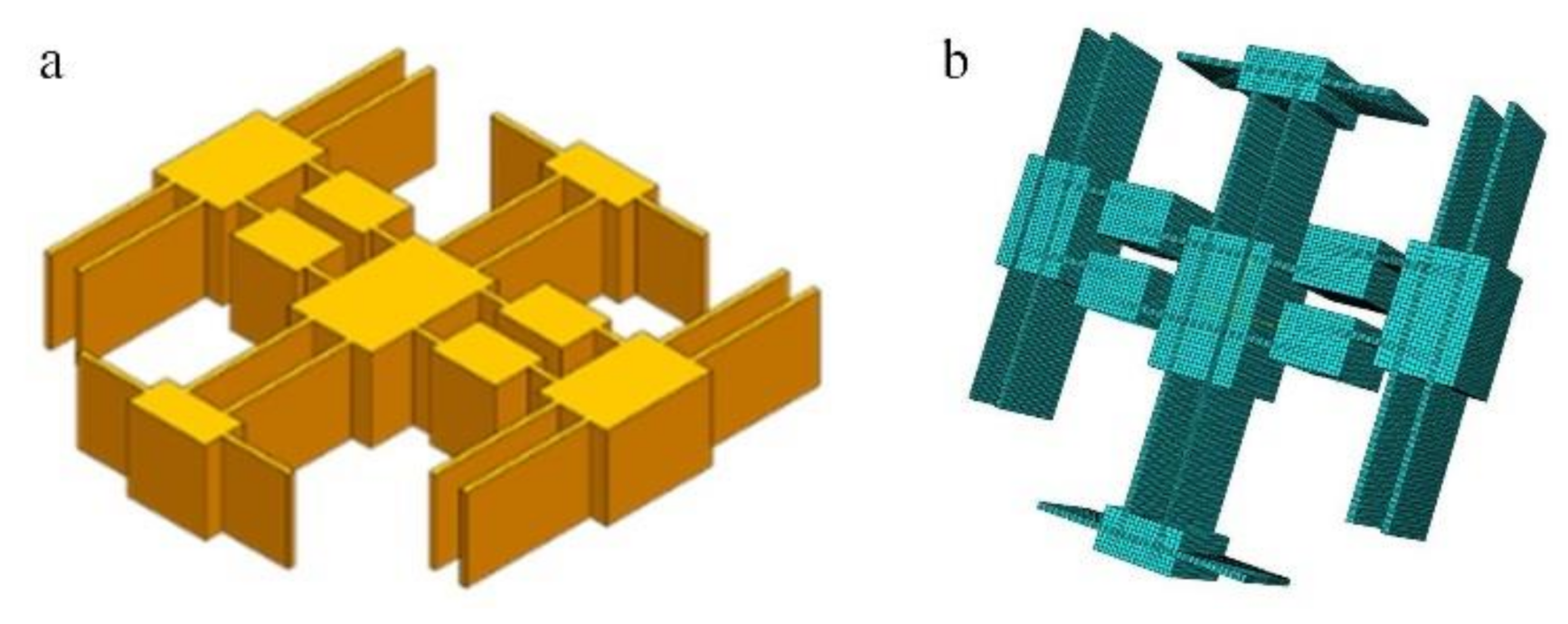
The stage was symmetrical along the Y-axis, and consisted of an output stage, double parallel rectangular beams, single rectangular beams, and displacement transmission units, while they were all on a rectangular beam hinge base. The two piezoelectric actuators were arranged symmetrically along the X-axis to realize the displacement input. The input displacement was transferred by displacement transmission units. Different working ranges were achieved via the cooperation of two piezoelectric actuators. Along the X-axis, double parallel rectangular beams and displacement transmission units added individual stiffness to improve the transmission stability of displacement input.

(2)

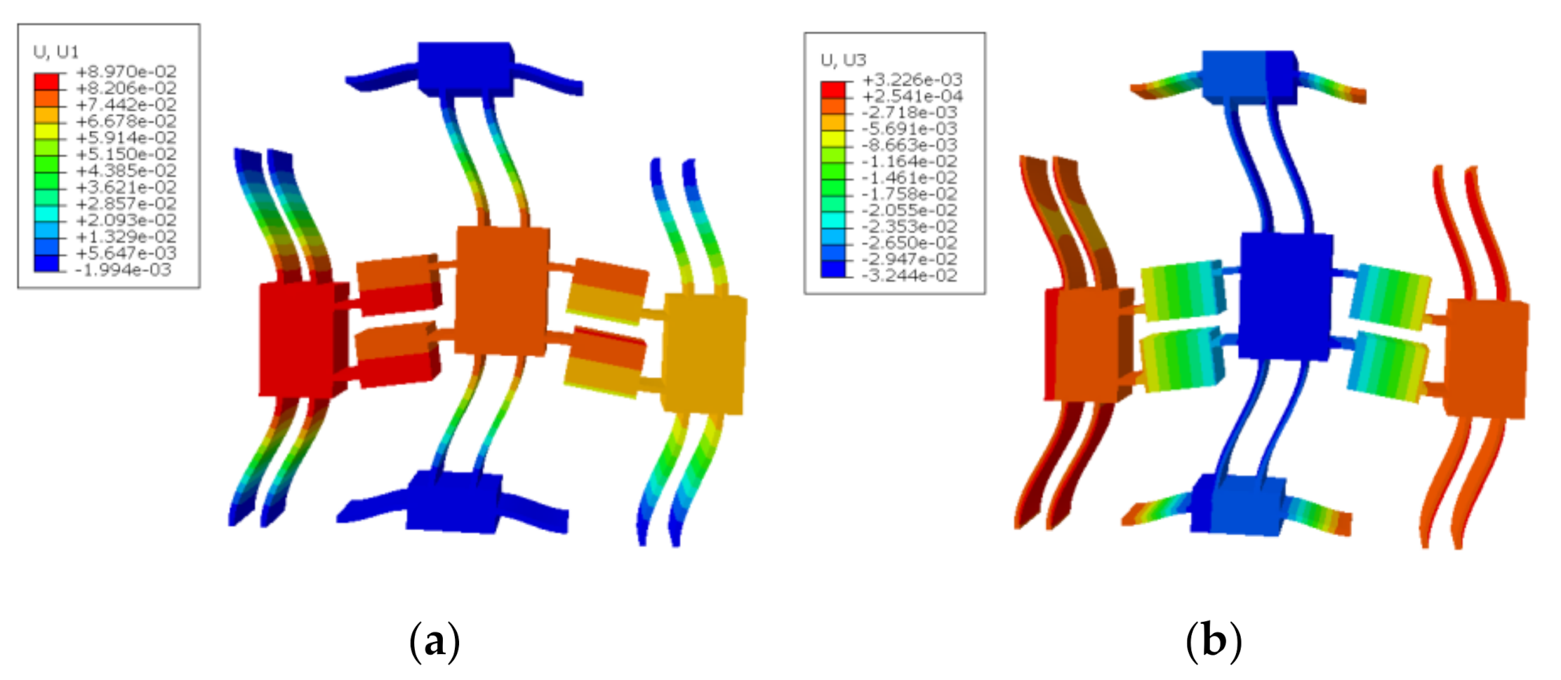
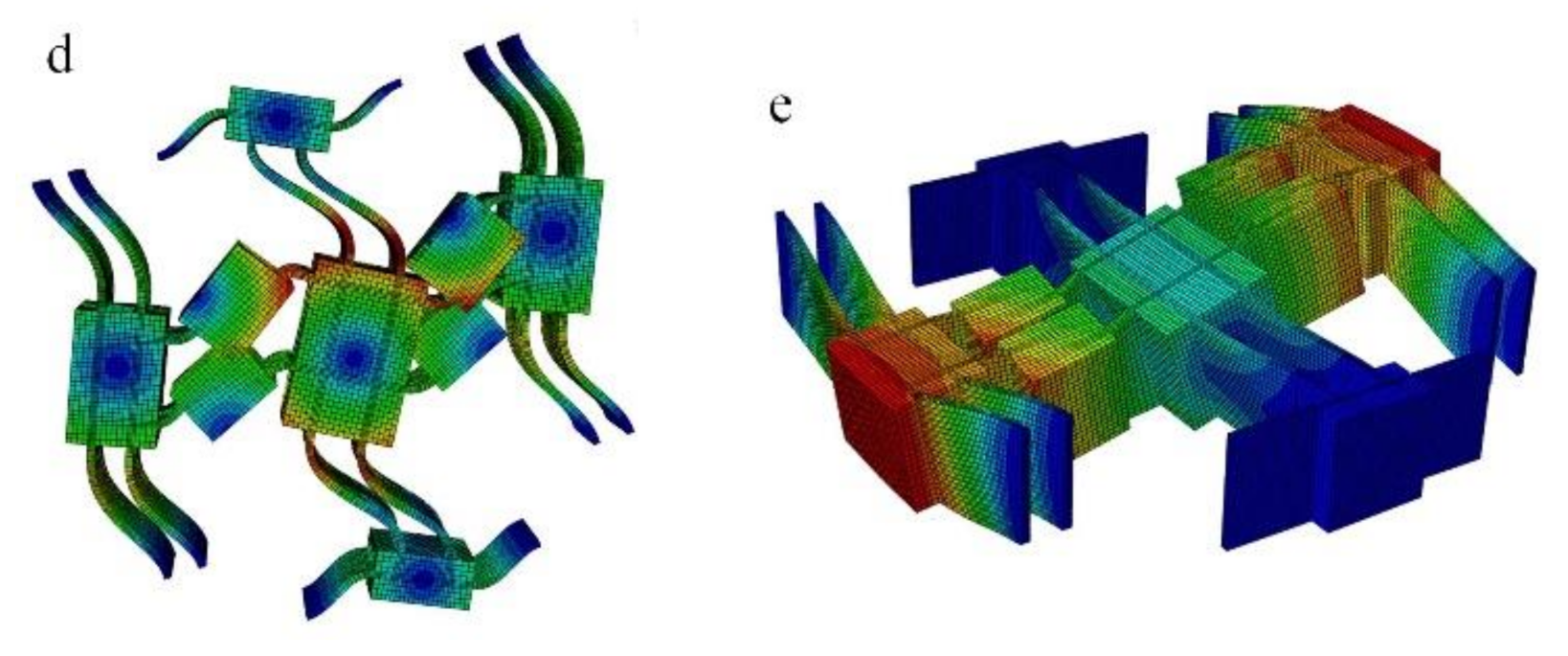
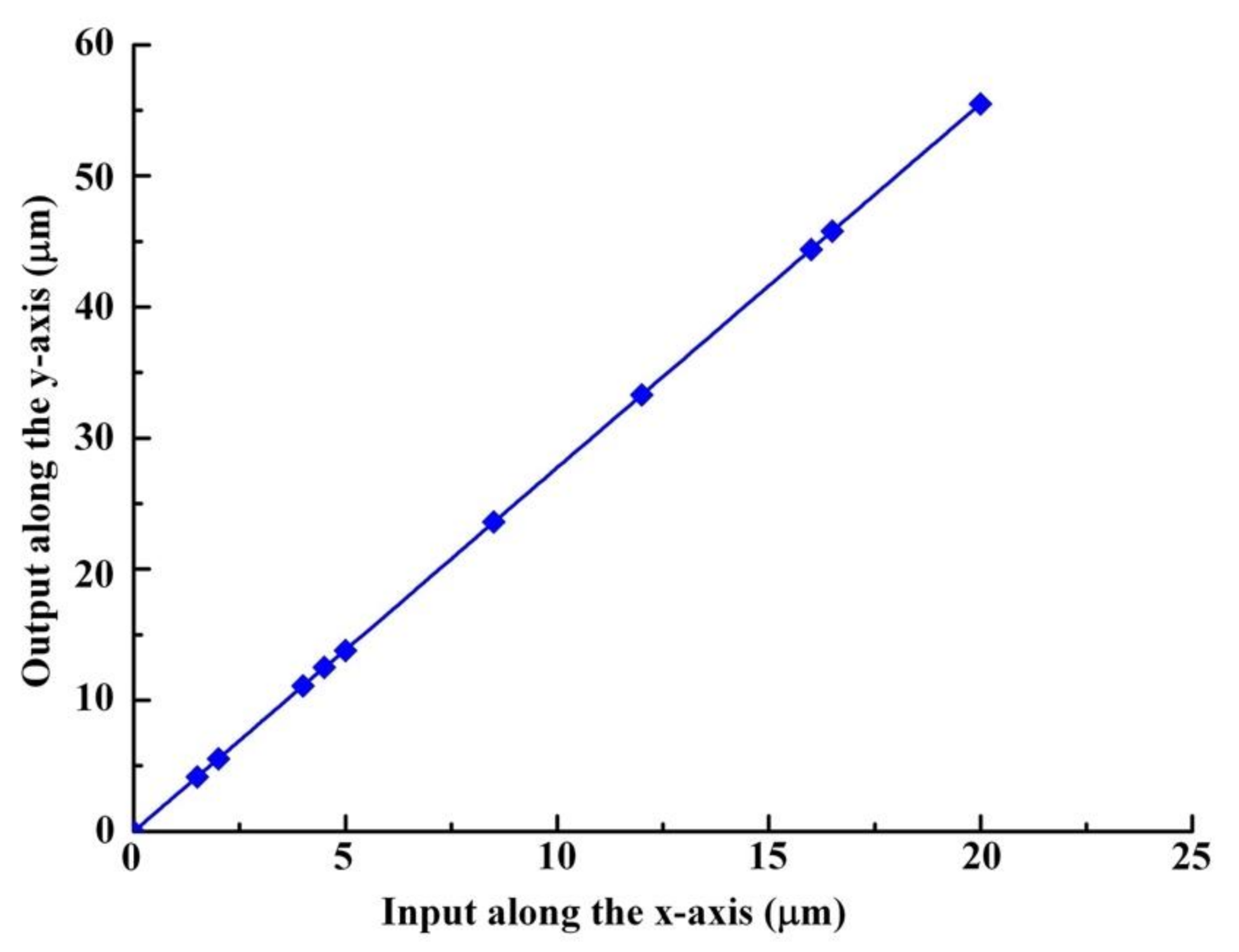
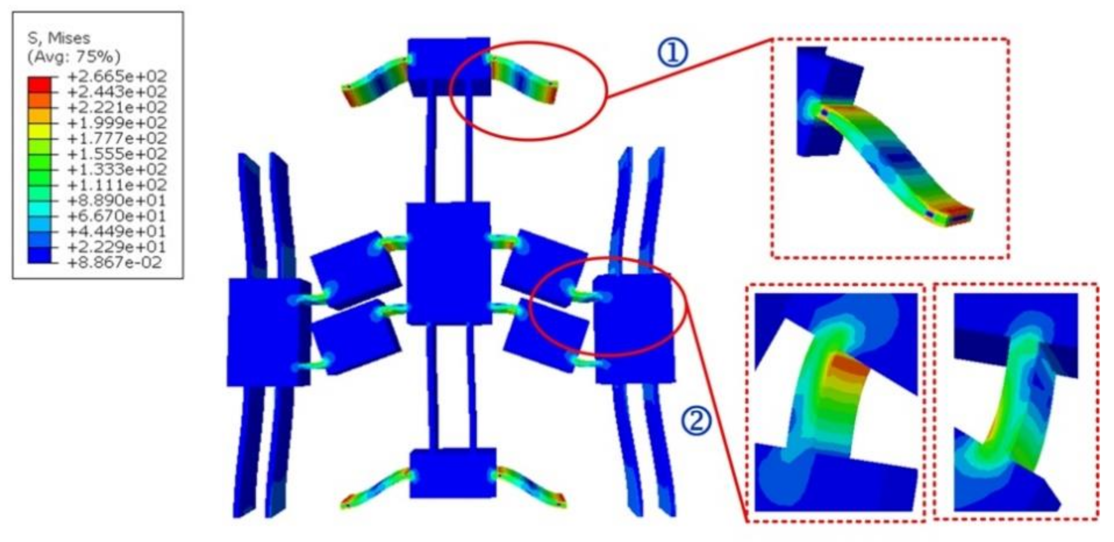
The compliance matrix method was used to establish an analytical model of the proposed positioning stage. The output stiffness in the X- and Y-directions were 1.34 μm/N and 0.438 μm/N. Finite element analysis was used to validate the theoretical equation. The error between the theoretical calculation and simulation analysis was within 2.2 and 5.3% in the X- and Y-directions, respectively. The frequency of the X- and Y-directions were 1088.9 and 2240.1 Hz, respectively. When given only a single direction input, the displacement average error was 3.83% and the displacement ratio of the X- to Y-directions was 10.07%. When given double direction inputs, in the Y-axis, the stage could realize a better displacement magnification, where the magnification ratio was 2.77 and the coupling error was 1 × 10⁻⁵%. Using this input method, the positioning stage could be used as a great direction amplifier, while also increasing the positioning range.

(3)

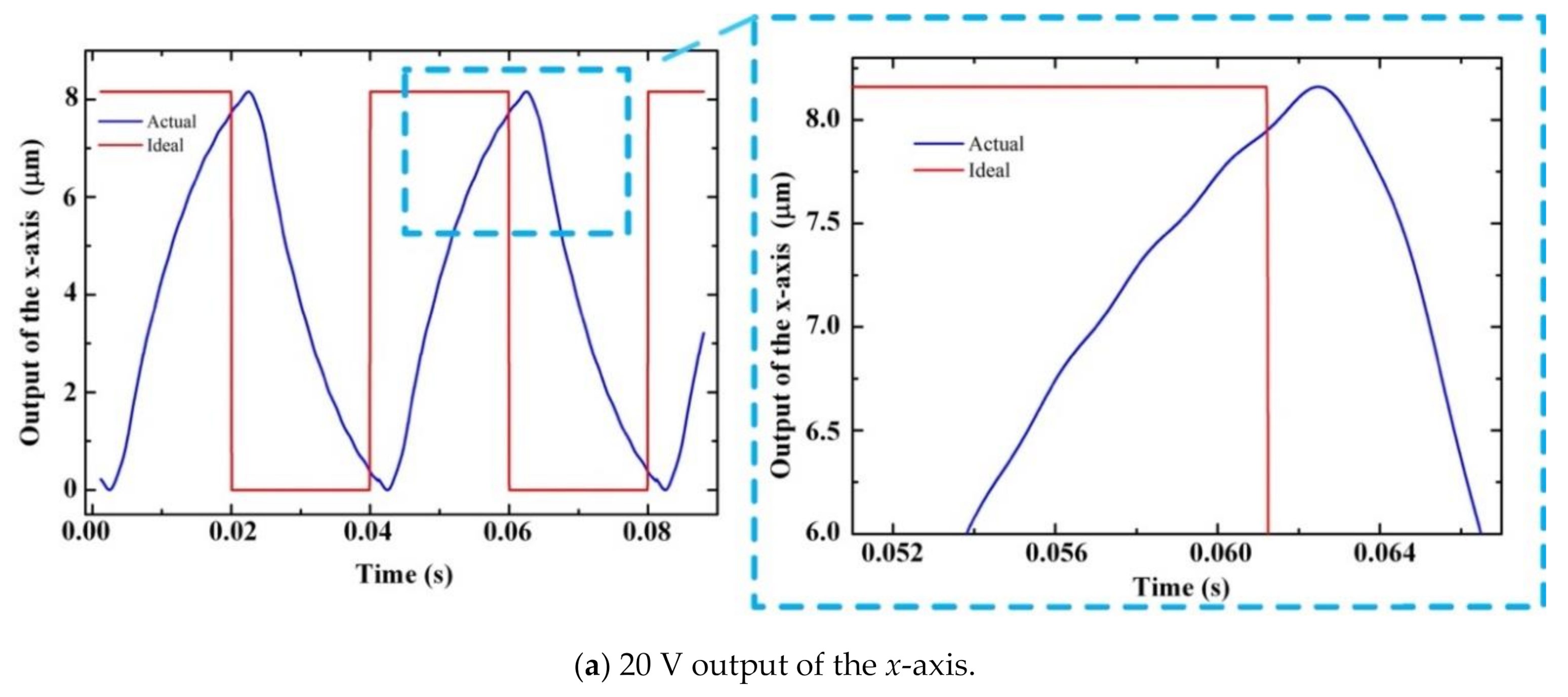
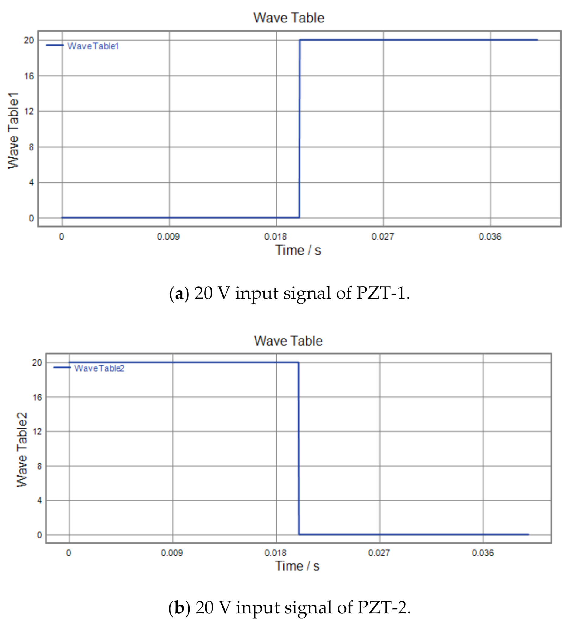
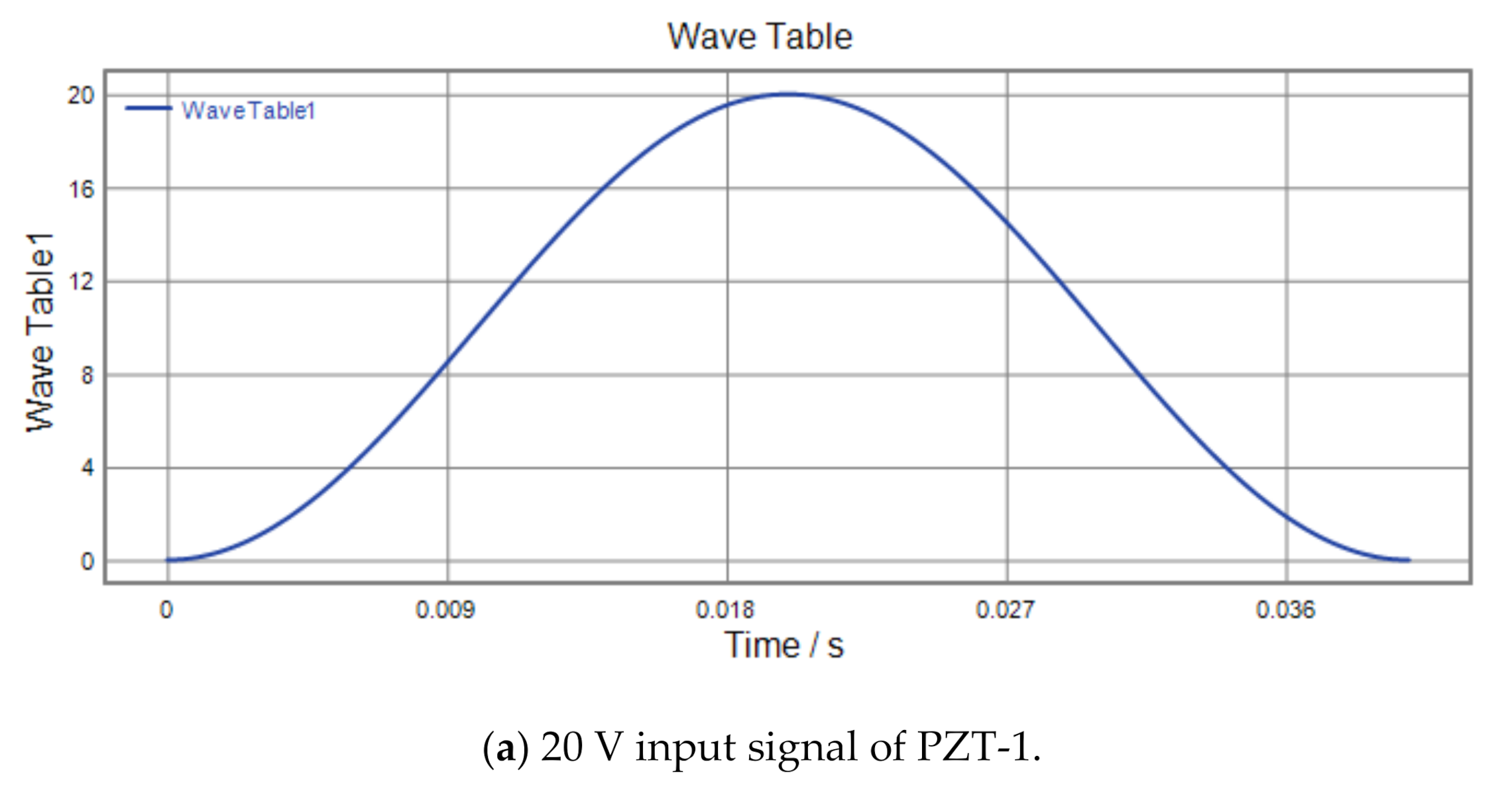
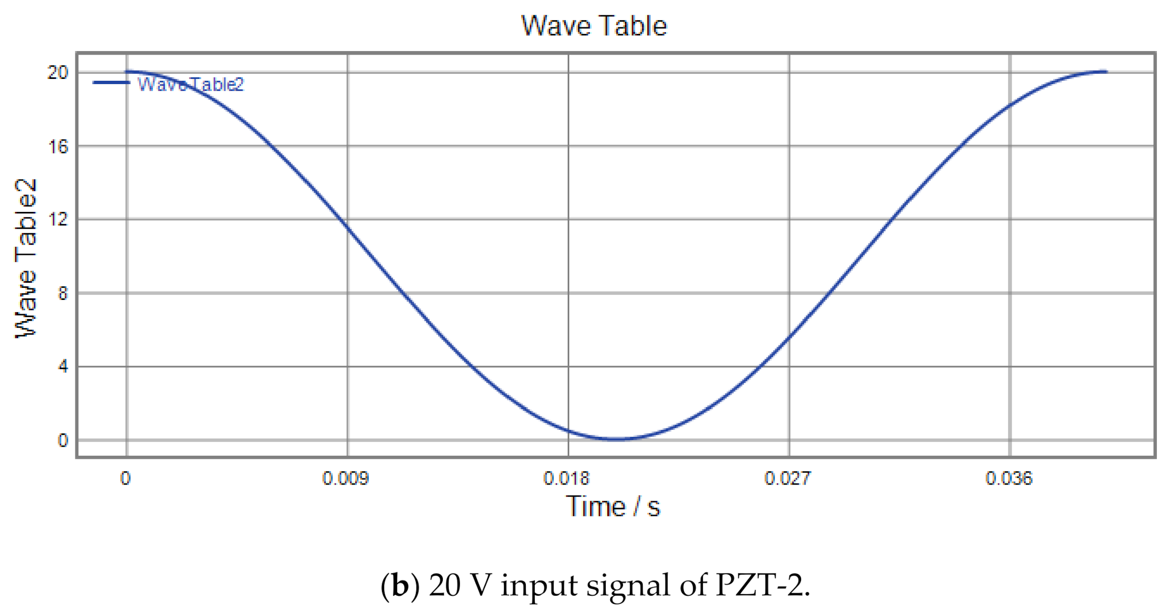
The performance evaluation of the mechanism was tested via experiments. The actual output signal tended to be flat after approximately 0.02 s. Along the X-axis, the initial position offset was approximately 0.084 μm and the maximum displacement difference caused by hysteresis was 1.11 μm. Along the Y-axis, the initial position offset was about 0.03 μm and the maximum displacement error was 0.3 μm. Under a certain safety factor and the stroke limit of the piezoelectric actuator, the maximum displacement in the X-direction was about 14.5 μm; the maximum displacement in the Y-direction was 6.97 μm. The experimental tests showed that the working range had an elliptical trajectory.

All the results indicated that the proposed stage possessed an ideal positioning property. Considering the practical requirements, more sizes and structures should be researched. Optimizations through algorithms should be carried out to improve the positioning property in the future.

References

- Sun, X.; Chen, W.; Fatikow, S.; Tian, Y.; Zhou, R.; Zhang, J.; Mikczinski, M. A novel piezo-driven microgripper with a large jaw displacement. Microsyst. Technol. 2015, 21, 931–942. [Google Scholar] [CrossRef]
- Qu, J.; Chen, W.; Zhang, J.; Chen, W. A large-range compliant micropositioning stage with remote-center-of-motion characteristic for parallel alignment. Microsyst. Technol. 2016, 22, 777–789. [Google Scholar] [CrossRef]
- Li, J.; Zhao, H.; Qu, X.; Qu, H.; Zhou, X.; Fan, Z.; Fu, H. Development of a compact 2-DOF precision piezoelectric positioning platform based on inchworm principle. Sens. Actuators A Phys. 2015, 222, 87–95. [Google Scholar] [CrossRef]
- Lee, H.J.; Woo, S.; Park, J.; Jeong, J.H.; Kim, M.; Ryu, J.; Gweon, D.G.; Choi, Y.M. Compact compliant parallel XY nano-positioning stage with high dynamic performance, small crosstalk, and small yaw motion. Microsyst. Technol. 2018, 24, 2653–2662. [Google Scholar] [CrossRef]
- Chen, W.; Qu, J.; Chen, W.; Zhang, J. A compliant dual-axis gripper with integrated position and force sensing. Mechatronics 2017, 47, 105–115. [Google Scholar] [CrossRef]
- Wang, N.; Zhang, Z.; Zhang, X.; Cui, C. Optimization of a 2-DOF micro-positioning stage using corrugated flexure units. Mech. Mach. Theory 2018, 121, 683–696. [Google Scholar] [CrossRef]
- Zhang, X.; Xu, Q. Design and testing of a new 3-DOF spatial flexure parallel micropositioning stage. Int. J. Precis. Eng. Manuf. 2018, 19, 109–118. [Google Scholar] [CrossRef]
- Noveanu, S.; Ivan, I.A.; Noveanu, D.C.; Rusu, C.; Lates, D. SiMFlex Micromanipulation Cell with Modular Structure. Appl. Sci. 2020, 10, 2861. [Google Scholar] [CrossRef]
- Cai, K.; He, X.; Tian, Y.; Liu, X.; Zhang, D.; Shirinzadeh, B. Design of a XYZ scanner for home-made high-speed atomic force microscopy. Microsyst. Technol. 2018, 24, 3123–3132. [Google Scholar] [CrossRef]
- Li, Y.; Xu, Q. A novel design and analysis of a 2-DOF compliant parallel micromanipulator for nanomanipulation. IEEE Trans. Autom. Sci. Eng. 2006, 3, 247–254. [Google Scholar]
- Jensen, K.A.; Lusk, C.P.; Howell, L.L. An XYZ Micromanipulator with Three Translational Degrees of Freedom. Robotica 2006, 24.3, 305–314. [Google Scholar] [CrossRef]
- Awtar, S.; Slocum, A.H. Constraint-Based Design of Parallel Kinematic XY Flexure Mechanisms. ASME J. Mech. Des. 2007, 129, 816–830. [Google Scholar] [CrossRef]
- Teo, T.J.; Yang, G.; Chen, I.M. A large deflection and high payload flexure-based parallel manipulator for UV nanoimprint lithography: Part I. Modeling and analyses. Precis. Eng. 2014, 38, 861–871. [Google Scholar] [CrossRef]
- Li, Y.; Xu, Q. A novel piezoactuated XY stage with parallel, decoupled, and stacked flexure structure for micro-/nanopositioning. IEEE Trans. Ind. Electron. 2010, 58, 3601–3615. [Google Scholar] [CrossRef]
- Xiao, S.; Li, Y.; Zhao, X. Design and analysis of a novel flexure-based XY micro-positioning stage driven by electromagnetic actuators. In Proceedings of the 2011 International Conference on Fluid Power and Mechatronics, Beijing, China, 17–20 August 2011; pp. 953–958. [Google Scholar]
- Kang, B.H.; Wen, J.Y.; Dagalakis, N.G.; Gorman, J.J. Analysis and design of parallel mechanisms with flexure joints. IEEE Trans. Robot. 2005, 21, 1179–1185. [Google Scholar] [CrossRef]
- Choi, K.B.; Kim, D.H. Monolithic parallel linear compliant mechanism for two axes ultraprecision linear motion. Rev. Sci. Instrum. 2006, 77, 065106. [Google Scholar] [CrossRef]
- DiBiasio, C.M.; Culpepper, M.L.; Panas, R.; Howell, L.L.; Magleby, S.P. Comparison of molecular simulation and pseudo-rigid-body model predictions for a carbon nanotube–based compliant parallel-guiding mechanism. J. Mech. Des. 2008, 130, 1–7. [Google Scholar] [CrossRef]
- Yong, Y.K.; Lu, T.F. Kinetostatic modeling of 3-RRR compliant micro-motion stages with flexure hinges. Mech. Mach. Theory 2009, 44, 1156–1175. [Google Scholar] [CrossRef]
- Liaw, H.C.; Shirinzadeh, B. Constrained motion tracking control of piezo-actuated flexure-based four-bar mechanisms for micro/nano manipulation. IEEE Trans. Automat. Sci. Eng. 2010, 7, 699–705. [Google Scholar] [CrossRef]
- Xue, G.; Toda, M.; Ono, T. Comb-drive XYZ-microstage based on assembling technology for low temperature measurement systems. In Proceedings of the 2015 International Conference on Electronics Packaging and iMAPS All Asia Conference (ICEP-IAAC), Kyoto, Japan, 14–17 April 2015; pp. 83–88. [Google Scholar]
- Khan, M.U.; Prelle, C.; Lamarque, F.; Büttgenbach, S. Design and assessment of a micropositioning system driven by electromagnetic actuators. IEEE/ASME Trans. Mechatron. 2016, 22, 551–560. [Google Scholar] [CrossRef]
- Lai, L.J.; Zhu, Z.N. Design, modeling and testing of a novel flexure-based displacement amplification mechanism. Sens. Actuators A: Phys. 2017, 266, 122–129. [Google Scholar] [CrossRef]
- Lin, C.; Shen, Z.; Wu, Z.; Yu, J. Kinematic characteristic analysis of a micro-/nano positioning stage based on bridge-type amplifier. Sens. Actuators A Phys. 2018, 271, 230–242. [Google Scholar] [CrossRef]
- Jiang, Y.; Li, T.; Wang, L.; Chen, F. Systematic Design Method and Experimental Validation of a 2-DOF Compliant Parallel Mechanism with Excellent Input and Output Decoupling Performances. Appl. Sci. 2017, 7, 591. [Google Scholar] [CrossRef]
- Jieqiong, L.; Jinguo, H.; Mingming, L.; Yan, G.; Wenhui, Z. Development of nonresonant elliptical vibration cutting device based on parallel piezoelectric actuator. Aip Adv. 2017, 7, 035304. [Google Scholar] [CrossRef]
- Wang, P.; Xu, Q. Design of a flexure-based constant-force XY precision positioning stage. Mech. Mach. Theory 2017, 108, 1–13. [Google Scholar] [CrossRef]
- Arata, J.; Kogiso, S.; Sakaguchi, M.; Nakadate, R.; Oguri, S.; Uemura, M.; Byunghyun, C.; Akahoshi, T.; Ikeda, T.; Hashizume, M. Articulated minimally invasive surgical instrument based on compliant mechanism. Int. J. Comput. Assist. Radiol. Surg. 2015, 10, 1837–1843. [Google Scholar] [CrossRef]
- Wang, P.; Xu, Q. Design of a flexure-based XY precision positioning stage with constant force output. In Proceedings of the IECON 2016-42nd Annual Conference of the IEEE Industrial Electronics Society, Florence, Italy, 23–26 October 2016; pp. 524–529. [Google Scholar]
- Wu, Y.; Zhou, Z. Design calculations for flexure hinges. Rev. Sci. Instrum. 2002, 73, 3101–3106. [Google Scholar] [CrossRef]
- Xu, Q. A novel compliant micropositioning stage with dual ranges and resolutions. Sens. Actuators A Phys. 2014, 205, 6–14. [Google Scholar] [CrossRef]
- Trease, B.P.; Moon, Y.-M.; Kota, S. Design of Large-Displacement Compliant Joints. J. Mech. Design. 2005, 127, 788–798. [Google Scholar] [CrossRef]
- Schotborgh, W.O.; Kokkeler, F.G.; Tragter, H.; Van Houten, F.J. Dimensionless design graphs for flexure elements and a comparison between three flexure elements. Precis. Eng. 2005, 29, 41–47. [Google Scholar] [CrossRef]
- Paros, J.M.; Weisboro, L. How to design flexure hinges. Mach. Des. 1965, 37, 151–157. [Google Scholar]
- Lobontiu, N. Compliant Mechanisms: Design of Flexure Hinges; CRC Press: Boca Raton, FL, USA, 2002. [Google Scholar]
- Xie, Y.; Li, Y.; Cheung, C.F.; Zhu, Z.; Chen, X. Design and analysis of a novel compact XYZ parallel precision positioning stage. Microsyst. Technol. 2020, 26, 1–8. [Google Scholar] [CrossRef]
- Lobontiu, N. Modeling and design of planar parallel-connection flexible hinges for in- and out-of-plane mechanism applications. Precis. Eng. 2015, 42, 113–132. [Google Scholar] [CrossRef]
- Lin, C.Y.; Po-Ying, C. Precision motion control of a nano stage using repetitive control and double-feedforward compensation. In Proceedings of the SICE Annual Conference, Taipei, Taiwan, 18–21 August 2010; pp. 22–29. [Google Scholar]
- Čeponis, A.; Mazeika, D. An inertial piezoelectric plate type rotary motor. Sens. Actuators A Phys. 2017, 263, 131–139. [Google Scholar] [CrossRef]
- Gu, G.-Y.; Zhu, L.-M.; Su, C.-Y.; Ding, H. Motion Control of Piezoelectric Positioning Stages: Modeling, Controller Design, and Experimental Evaluation. IEEE/ASME Trans. Mechatron. 2012, 18, 1459–1471. [Google Scholar] [CrossRef]
- Yuan, S.; Zhao, Y.; Chu, X.; Zhu, C.; Zhong, Z. Analysis and Experimental Research of a Multilayer Linear Piezoelectric Actuator. Appl. Sci. 2016, 6, 225. [Google Scholar] [CrossRef]
- Jia, S.; Jiang, Y.; Li, T.; Du, Y. Learning-Based Optimal Desired Compensation Adaptive Robust Control for a Flexure-Based Micro-Motion Manipulator. Appl. Sci. 2017, 7, 406. [Google Scholar] [CrossRef]
- Choi, K.-B.; Lee, J.J.; Hata, S. A piezo-driven compliant stage with double mechanical amplification mechanisms arranged in parallel. Sens. Actuators A Phys. 2010, 161, 173–181. [Google Scholar] [CrossRef]