The Influence of Pillar Displacements on Geodetic Measurements

Abstract

This paper deals with the effects that displacements of the measuring pillar have on precise geodetic measurements. The changes in the position of the control points on the object or its surroundings can only be determined with well stabilized and stable reference points. These points are usually stabilized with measuring pillars which are not always constructed in an optimal manner. If they are placed in a dark tube with a high absorption factor, solar heating on one side of the pillar can cause the pillar to deflect considerably due to the temperature difference on the two sides of the pillar. This paper presents the influence of such a displacement, if the pillar is a survey point, orientation point, or control point. We show that even small displacement of the survey point can have important influence on all measurements and that the error in some cases significantly increases, e.g., if the standard deviations of the coordinates of the survey point are 1 mm and their covariance is assumed to be zero, the standard deviation of the distance between measured and exact position of the control point exceeds the value of 2.2 mm.

1. Introduction

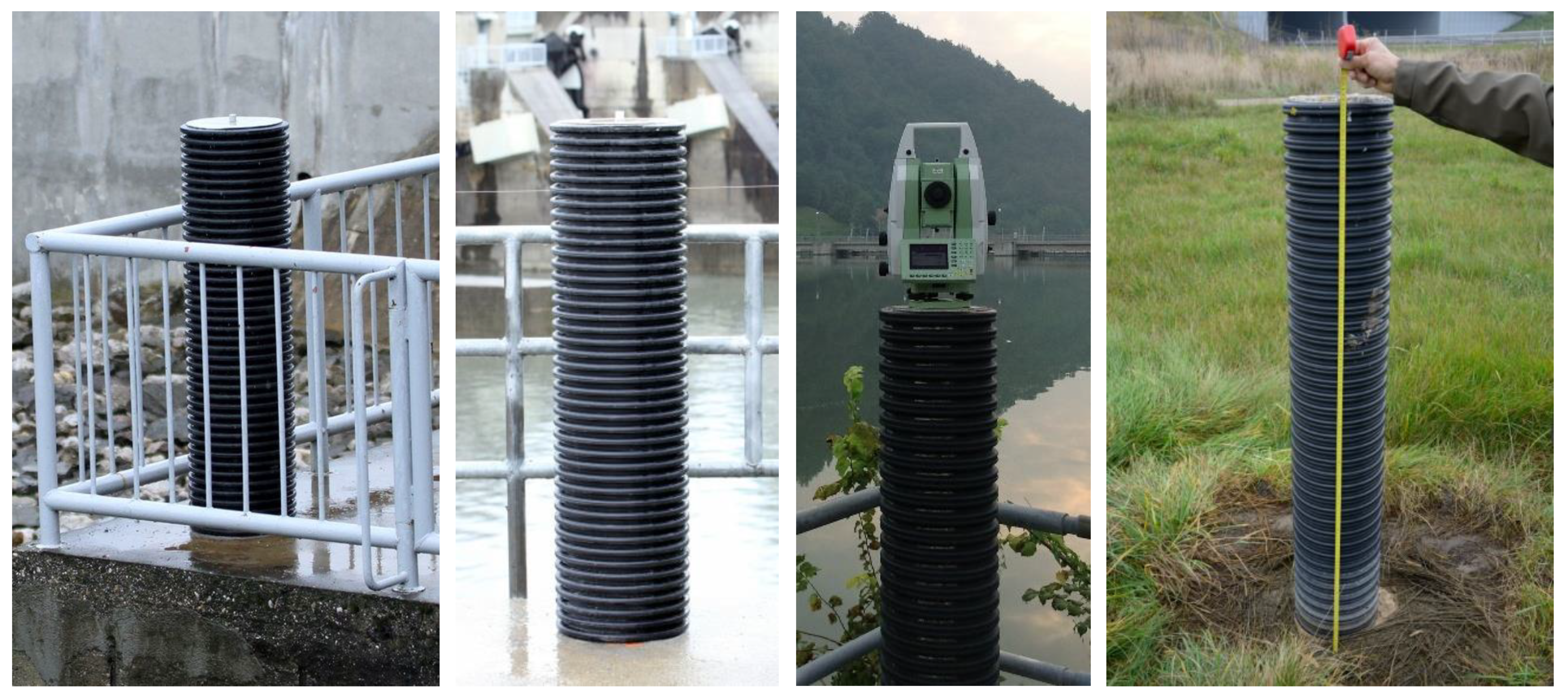
We cannot afford to make gross errors in precise geodetic measurements or in defining the coordinates of reference points or points with a size of around 1 mm. Therefore, we try to eliminate or at least reduce systematic errors by comparing instruments, using appropriate measuring methods, taking into account the meteorological conditions in the environment, etc. [1]. However, there are certain sources of errors present that are hard to avoid. Systematic errors include the deflection of the measuring pillar, which can occur due to the variation of the temperature field inside the pillar; especially when the sun shines on one side and the other side is in the shadow. This results in temperature differences inside the pillar body, which are considered as a temperature load and lead to deformations of the pillar. If the pillar is improperly stabilized, i.e., if a small-diameter reference pillar and a dark drain tube with a high absorption factor are used for stabilization (Figure 1), the deformations are considerable and cannot be neglected.

Based on calculations [2] and an experiment [3] we have established that a temperature difference of 16.2 °C between the two sides of a 1.5 m high pillar results in displacements of the screw for forced centering of the instrument of magnitudes around 1 mm, which is a considerable displacement for precise measurements. In the experiment, a ribbed tube was used made of plastic material with an outer diameter of 250 mm and an inner diameter of 217 mm. A welded reinforcement was rolled in the form of a cylinder, installed into the tube, and then the tube was filled with concrete C25/30. The Dewetron system for data capturing and the Agilent VEE Pro application were used to gather data from the thermocouple wire. The measurements are precise up to 0.3 K. For more details and the comparisons among other measurement error sources, the reader is referred to paper [3].

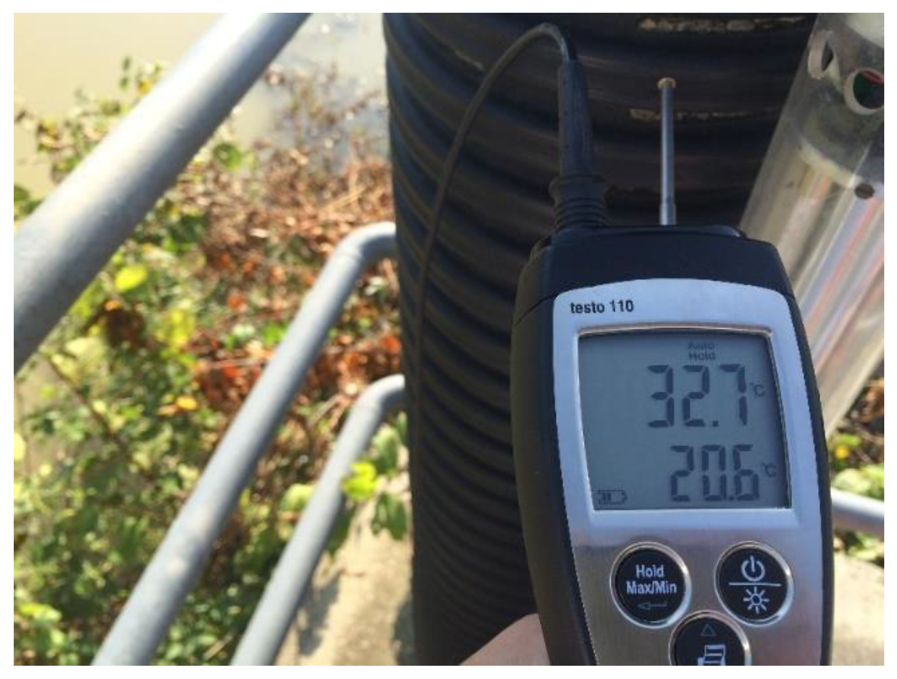
The photograph in Figure 2 shows a measurement we made on site, without waiting for extreme conditions. The photograph shows the temperatures measured on the sunny and shady side of the pillar.

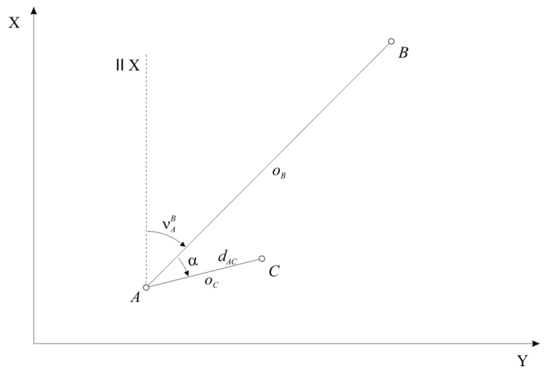
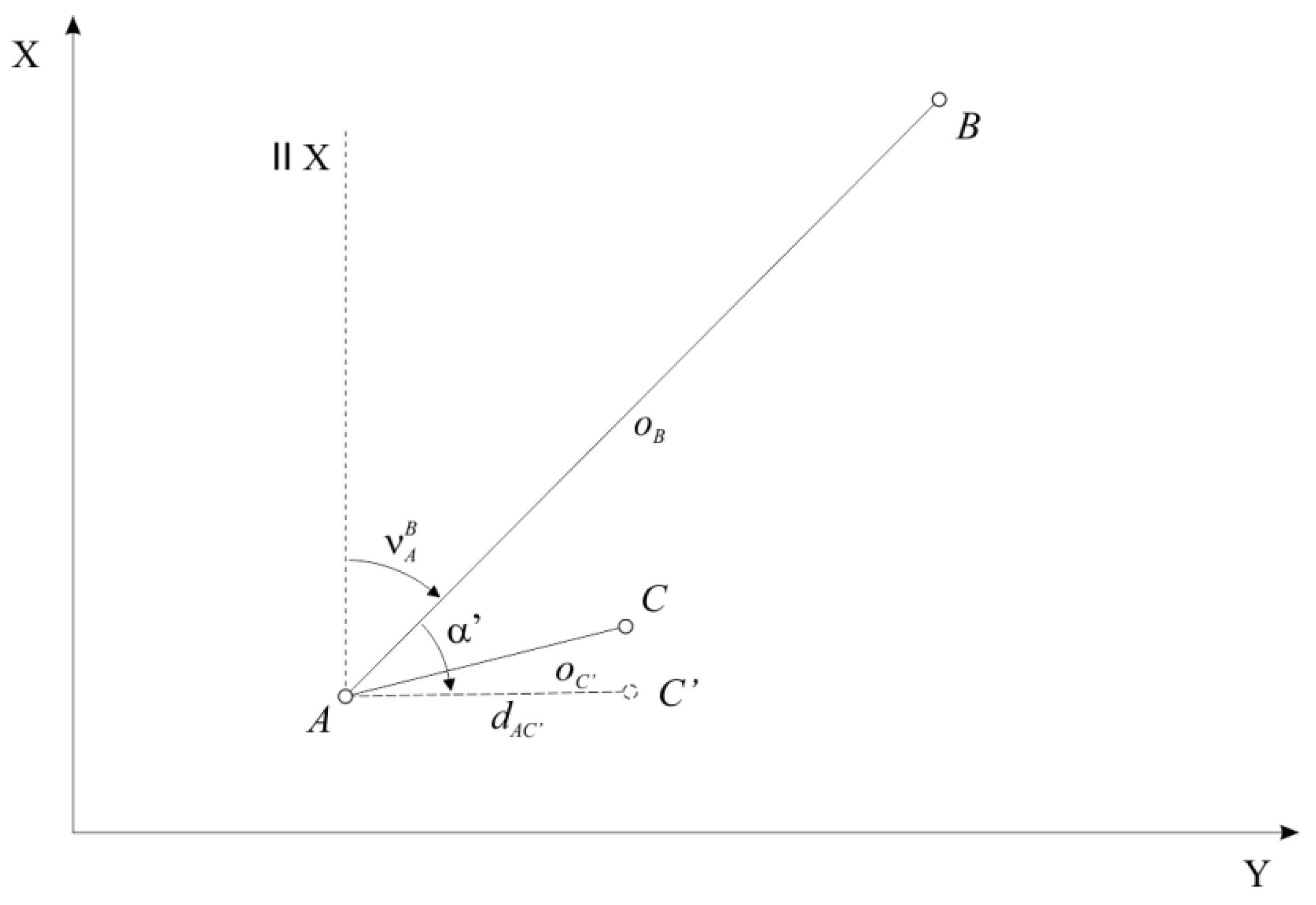
In this paper, we discuss how much the displacements of the pillar, which occur as a result of a temperature variation along the pillar body, could affect the control point on the object when the displacement occurs at the orientation point, survey point, or control point. The influence of the displacement is analyzed using a simple example of a measurement performed using the polar method (Figure 3), where we have measured the horizontal direction $o_B$ from reference point $A$ (survey point) to the second reference point $B$ (orientation point) as well as the horizontal direction $o_C$ and the distance $d_{AC}$ of the control point $C$. The horizontal angle $\alpha$ is calculated as the difference between the measured horizontal directions [4]:

$$\alpha =o_C-o_B.$$

(1)

The bearing between the reference points $A$ and $B$ is calculated as follows:

$$\tan {\nu }_A^B=\frac{y_B-y_A}{x_B-x_A}=\frac{\mathsf{\Delta }{y}_A^B}{\mathsf{\Delta }{x}_A^B},$$

(2)

while the bearing to the control point $C$ is calculated as:

$${\nu }_A^C={\nu }_A^B+\alpha .$$

(3)

The coordinates of control point $C$ are calculated as follows:

$$y_C=y_A+\mathsf{\Delta }{y}_A^C=y_A+d_{AC}·\sin {\nu }_A^C\mathrm{and}$$

(4)

$$x_C=x_A+\mathsf{\Delta }{x}_A^C=x_A+d_{AC}·\cos {\nu }_A^C.$$

(5)

Literature (let us name only a few sources: [5,6,7,8,9,10]) deals with the influence of the displacement of the signalized points (in our case, the displacement of points $B$ and $C$) and the influence of the centering error (in our example, the displacement of point $A$) on the measured horizontal angles; in our paper, we will discuss the influence of these displacements on the position of the control point, i.e., on the coordinates of the control point.

2. The Analysis of the Influence Temperature Displacements of a Pillar on the Position of the Control Point

First of all, we need to look at the law of propagation of variances and covariances, as we will use this law in what follows. Then, we will discuss the influence of the temperature displacement of the pillar on the determination of the coordinates of the control point on the object, if such a pillar is an orientation point, a survey point, or the control point on the object.

2.1. Linearization

The relations between the geodetic measurements and other parameters are usually described by non-linear functions. For practical applications, non-linear functions are often (at least locally) approximated by the linear ones. Starting from a Taylor series expansion [11] of a non-linear function $\mathit{y}=\mathit{F}\left(\mathit{x}\right)=\left[\begin{array}{c}{F}_1\left(\mathit{x}\right)\\ ⋮\\ F_n\left(\mathit{x}\right)\end{array}\right]=\left[\begin{array}{c}{F}_1\left(x_1,x_2,\dots x_u\right)\\ ⋮\\ F_n\left(x_1,x_2,\dots x_u\right)\end{array}\right]$ about the point ${\mathit{x}}_0$:

$$\mathit{y}=\mathit{F}\left({\mathit{x}}_0\right)+{D\mathit{F}|}_{\mathit{x}={\mathit{x}}_0}\left(\mathit{x}-{\mathit{x}}_0\right)+\frac{1}{2!}{\left(\mathit{x}-{\mathit{x}}_0\right)}^T{D^2\mathit{F}|}_{\mathit{x}={\mathit{x}}_0}\left(\mathit{x}-{\mathit{x}}_0\right)+\cdots ,$$

(6)

where $D\mathit{F}=\left[\begin{array}{ccc}\frac{\partial F_1}{\partial x_1}& \cdots & \frac{\partial F_1}{\partial x_u}\\ ⋮& \ddots & ⋮\\ \frac{\partial F_n}{\partial x_1}& \cdots & \frac{\partial F_n}{\partial x_u}\end{array}\right]$ denotes the Jacobian matrix of first-order partial derivatives, $D^2\mathit{F}$ denotes the Hessian matrix of second order partial derivatives, while in higher-order terms, the higher order partial derivatives are present.

When we neglect the higher-order terms and take only the linear part:

$$\overline{\mathit{y}}=\mathit{F}\left({\mathit{x}}_0\right)+{D\mathit{F}|}_{\mathit{x}={\mathit{x}}_0}\left(\mathit{x}-{\mathit{x}}_0\right),$$

(7)

we get a linear function, which coincides with the original one at ${\mathit{x}}_0$ and represents an approximation of the original one $\mathit{y}=\mathit{F}\left(\mathit{x}\right).$ Note that the error of approximation is strongly dependent on the distance between $\mathit{x}$ and ${\mathit{x}}_0$ and that in general such approximation makes sense only in a close neighbourhood to ${\mathit{x}}_0$.

2.2. Law of Propagation of Variances and Covariances

There are two ways to calculate the precision of estimates of the calculated quantity. If we have redundant measurements, we can calculate the most likely value of the desired quantity and adjust its precision. If we have just enough measurements, we can calculate the desired quantity monotonically, and then estimate its precision by applying the law of propagation of variances and covariances [12].

In the following, we will consider all the parameters to be random variables. We will focus on the expected value of the parameter described by a random variable $X_i$ and its standard deviation ${\sigma }_{X_i}$, which reveals the dispersity of the parameter. The expected value ${\mu }_{X_i}$ of a random variable $X_i$ is evaluated using the following equation [11]:

$${\mu }_{X_i}=\mathrm{E}\left[X_i\right]={\int }_{-\infty }^{\infty }\dots {\int }_{-\infty }^{\infty }{x}_i{\mathit{f}}_{\mathit{X}}\left(x_1,x_2,\dots ,x_n\right)d{x}_1\cdots d{x}_n,$$

(8)

where ${\mathit{f}}_{\mathit{X}}\left(x_1,x_2,\dots ,x_n\right)$ denotes the probability density function of the random vector X consisting of all random variables of the problem. With respect to the primary axioms of probability, ${\mathit{f}}_{\mathit{X}}$ is strictly positive and its integral is equal to one.

The variance ${\sigma }_{X_i}^2$ of a random variable $X_i$ is calculated using [11]:

$${\sigma }_{X_i}^2=\mathrm{E}\left[{\left(X_i-{\mu }_{x_i}\right)}^2\right]={\int }_{-\infty }^{\infty }\dots {\int }_{-\infty }^{\infty }{\left(x_i-{\mu }_{x_i}\right)}^2{\mathit{f}}_{\mathit{X}}\left(x_1,x_2,\dots ,x_n\right)d{x}_1\cdots d{x}_n,$$

(9)

while the standard deviation defined as:

$${\sigma }_{X_i}=\sqrt{{\sigma }_{X_i}^2}.$$

(10)

For any two components of a random vector, we can also calculate the covariance, which describes the statistical correlation between two random variables. The covariance is calculated as follows [11]:

$$\begin{gathered} {\sigma }_{X_i{X}_j}=\mathrm{E}\left[\left(X_i-{\mu }_{X_i}\right)\left(X_j-{\mu }_{X_j}\right)\right]={\int }_{-\infty }^{\infty }\dots {\int }_{-\infty }^{\infty }\left(x_i-{\mu }_{x_i}\right) \\ \left(x_j-{\mu }_{x_j}\right){\mathit{f}}_{\mathit{X}}\left(x_1,x_2,\dots ,x_n\right)d{x}_1\cdots d{x}_n, \end{gathered}$$

(11)

while the variance is always positive, the covariance can be negative.

For any random vector of size $n$, we can calculate the variances for each component using Equation (9) and the covariances for each pair of components according to Equation (11). The results can be written in the form called variance-covariance matrix [11]:

$${\Sigma }_{\mathit{X}\mathit{X}}=\mathrm{E}\left[\left(\mathit{X}-{\mathit{\mu }}_{\mathit{X}}\right){\left(\mathit{X}-{\mathit{\mu }}_{\mathit{X}}\right)}^{\mathrm{T}}\right]=\left[\begin{array}{ccc}{\sigma }_{X_1}^2& \cdots & {\sigma }_{X_1{X}_n}\\ ⋮& \ddots & ⋮\\ {\sigma }_{X_n{X}_1}& \cdots & {\sigma }_{X_n}^2\end{array}\right].$$

(12)

Note that ${\Sigma }_{\mathit{X}\mathit{X}}$ is a symmetrical, since ${\sigma }_{X_i{X}_j}={\sigma }_{X_j{X}_i},$ where $i,j=1,\dots ,n$.

Starting from a simple linear transformation of a random vector $\mathit{Y}={\mathit{J}}_{\mathbf{0}}+J·\mathit{X}$, where ${\mathit{J}}_{\mathbf{0}}$ is a vector of constants and $J$ the constant transformation matrix, we can find the following relation:

$${\Sigma }_{\mathit{Y}\mathit{Y}}=J·{\Sigma }_{\mathit{X}\mathit{X}}·J^{\mathrm{T}},$$

(13)

where ${\Sigma }_{\mathit{Y}\mathit{Y}}$ is a variance-covariance matrix of a vector. Equation (13) is called the law of propagation of variances and covariances between the random vectors $\mathit{X}$ and $\mathit{Y}$.

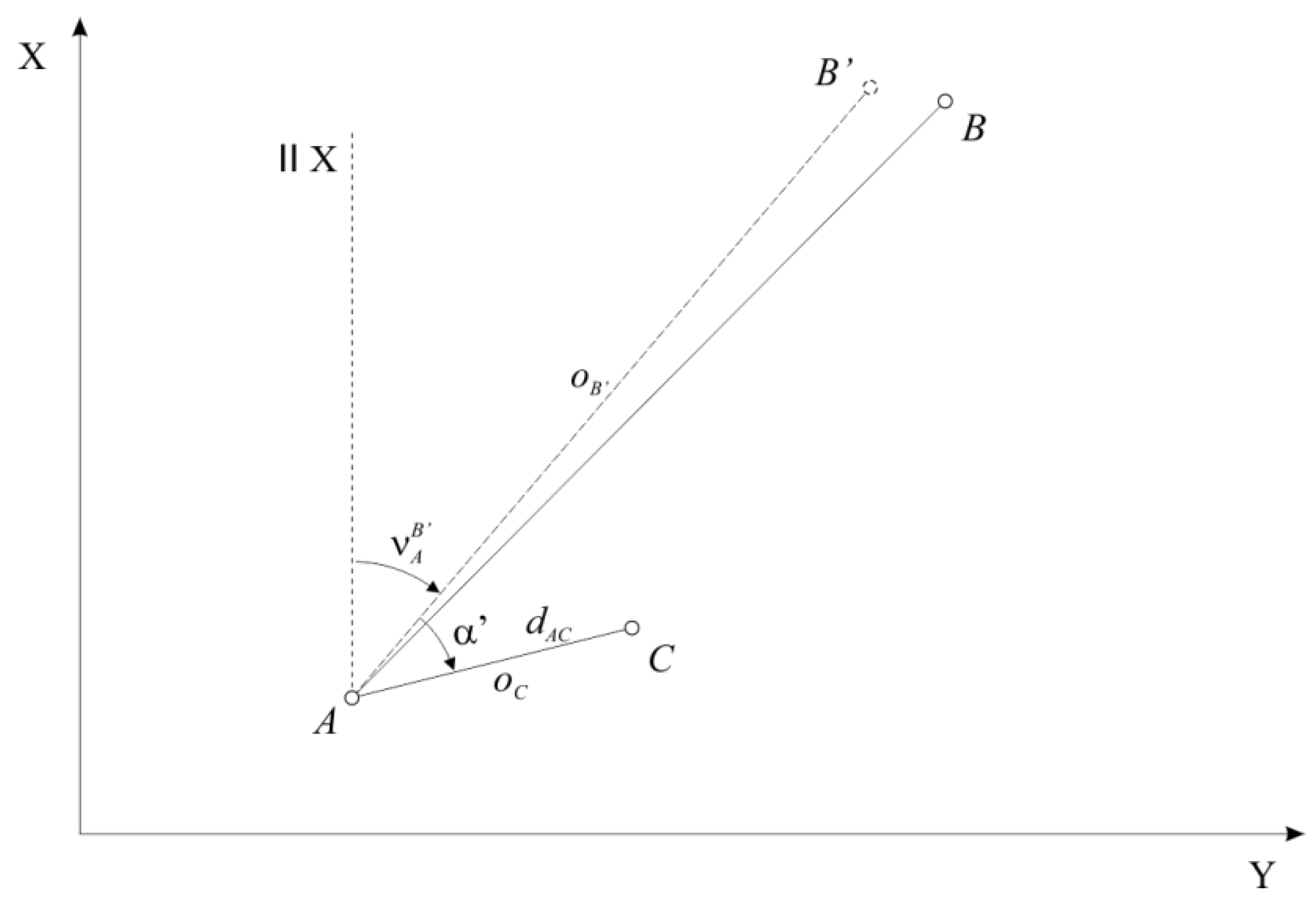
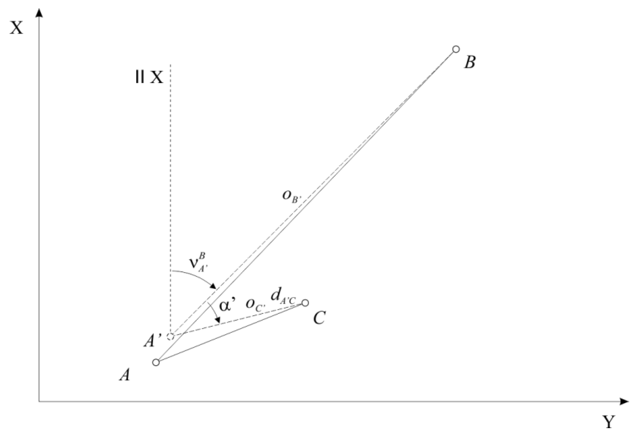
2.3. The Influence of the Temperature Displacements at Orientation Point $B$ on the Position of the Control Point $C$

If the temperature load displaces the position of the orientation point $B$, we use the point $B^{\prime }\left(y_{B^{\prime }},x_{B^{\prime }}\right)$, instead of the point $B\left(y_B,x_B\right)$ for our measurements. The two points are related by $y_{B^{\prime }}=y_B+{\delta }_{y_B}$ and $x_{B^{\prime }}=x_B+{\delta }_{x_B}$, where ${\delta }_{y_B}$ and ${\delta }_{x_B}$ represent the displacements of the position of point $B$ (Figure 4). Consequently, we measure the horizontal angle ${\alpha }^{\prime }=\alpha +{\delta }_{\alpha }$, where ${\delta }_{\alpha }$ is the error of the horizontal angle $\alpha$, instead of measuring horizontal angle $\alpha$. The horizontal angle ${\alpha }^{\prime }$ is calculated as the difference between the measured horizontal direction at control point $C$ and the (displaced) measured horizontal direction at orientation point $B^{\prime }$ [4]:

$${\alpha }^{\prime }=o_A^C-o_A^{B^{\prime }}.$$

(14)

Due to the displacement of the orientation point $B$, the horizontal angle $\alpha$ shows an error. Considering the approximations $y_{B^{\prime }}=y_B$ and $x_{B^{\prime }}=x_B,$ we can calculate the position of the control point $C$:

$$y_C=y_A+d_{AC}\sin \left({\nu }_A^B+{\alpha }^{\prime }\right)\mathrm{and}$$

(15)

$$x_C=x_A+d_{AC}\cos \left({\nu }_A^B+{\alpha }^{\prime }\right),$$

(16)

where $d_{AC}=\sqrt{{\left(y_C-y_A\right)}^2+{\left(x_C-x_A\right)}^2}$ is the distance between survey point $A$ and control point $C$, ${\nu }_A^B=\mathrm{atan}\frac{y_B-y_A}{x_B-x_A}$ denotes the displaced bearing between survey point $A$ and the displaced orientation point $B$.

We can express the position of the control point $C$ using the following two equations:

$${\mathrm{F}}_1\equiv y_C=y_A+d_{AC}\sin \left(\mathrm{atan}\frac{y_B-y_A}{x_B-x_A}+{\alpha }^{\prime }\right)\mathrm{and}$$

(17)

$${\mathrm{F}}_2\equiv x_C=x_A+d_{AC}\cos \left(\mathrm{atan}\frac{y_B-y_A}{x_B-x_A}+{\alpha }^{\prime }\right).$$

(18)

Observe, that the relation between the coordinates of these two points is non-linear and we will linearize it to be able to apply Equation (13). The Jacobian matrix in terms of coordinates of orientation point $B$ is as follows:

$$\frac{\partial {\mathrm{F}}_1}{\partial y_B}=d_{AC}\cos \left({\nu }_A^B+{\alpha }^{\prime }\right)·\frac{\mathsf{\Delta }{x}_A^B}{d_{AB}^2},$$

(19)

$$\frac{\partial {\mathrm{F}}_1}{\partial x_B}=-d_{AC}\cos \left({\nu }_A^B+{\alpha }^{\prime }\right)·\frac{\mathsf{\Delta }{y}_A^B}{d_{AB}^2},$$

(20)

$$\frac{\partial {\mathrm{F}}_2}{\partial y_B}=-d_{AC}\sin \left({\nu }_A^B+{\alpha }^{\prime }\right)·\frac{\mathsf{\Delta }{x}_A^B}{d_{AB}^2},\mathrm{and}$$

(21)

$$\frac{\partial {\mathrm{F}}_2}{\partial x_B}=d_{AC}\sin \left({\nu }_A^B+{\alpha }^{\prime }\right)·\frac{\mathsf{\Delta }{y}_A^B}{d_{AB}^2}.$$

(22)

Here, $\mathsf{\Delta }{y}_A^B=y_B-y_A$ and $\mathsf{\Delta }{x}_A^B=x_B-x_A$ are the coordinate differences between survey point $A$ and orientation point $B$, while $d_{AC}=\sqrt{{\left(y_C-y_A\right)}^2+{\left(x_C-x_A\right)}^2}$ is the distance between both points.

These component are then gathered in the matrix $J_B=\left[\begin{array}{cc}\frac{\partial {\mathrm{F}}_1}{\partial y_B}& \frac{\partial {\mathrm{F}}_1}{\partial x_B}\\ \frac{\partial {\mathrm{F}}_2}{\partial y_B}& \frac{\partial {\mathrm{F}}_2}{\partial x_B}\end{array}\right]$.

Starting from known (or assumed) standard deviations ${\sigma }_{y_B}$ and ${\sigma }_{x_B}$ and the covariance ${\sigma }_{x{y}_B}$ for the position of the orientation point $B\left(y_B,x_B\right)$, we can now evaluate standard deviations and covariance for the coordinates of the control point $C$ using Equation (13):

$${\Sigma }_{\mathit{X}{\mathit{X}}_C}=\left[\begin{array}{cc}{\sigma }_{y_C}^2& {\sigma }_{x{y}_C}\\ {\sigma }_{x{y}_C}& {\sigma }_{x_C}^2\end{array}\right]=J_B·{\Sigma }_{\mathit{X}{\mathit{X}}_B}·J_B^T=\left[\begin{array}{cc}\frac{\partial {\mathrm{F}}_1}{\partial y_B}& \frac{\partial {\mathrm{F}}_1}{\partial x_B}\\ \frac{\partial {\mathrm{F}}_2}{\partial y_B}& \frac{\partial {\mathrm{F}}_2}{\partial x_B}\end{array}\right]\left[\begin{array}{cc}{\sigma }_{y_B}^2& {\sigma }_{x{y}_B}\\ {\sigma }_{x{y}_B}& {\sigma }_{x_B}^2\end{array}\right]{\left[\begin{array}{cc}\frac{\partial {\mathrm{F}}_1}{\partial y_B}& \frac{\partial {\mathrm{F}}_1}{\partial x_B}\\ \frac{\partial {\mathrm{F}}_2}{\partial y_B}& \frac{\partial {\mathrm{F}}_2}{\partial x_B}\end{array}\right]}^{\mathrm{T}}.$$

(23)

After some algebra, we express:

$${\sigma }_{y_C}^2=\frac{d_{AC}^2}{d_{AB}^4}·{\cos }^2\left({\nu }_A^B+{\alpha }^{\prime }\right)·\left(\mathsf{\Delta }{x}_A^B·\mathsf{\Delta }{x}_A^B·{\sigma }_{y_B}^2-2\mathsf{\Delta }{y}_A^B·\mathsf{\Delta }{x}_A^B·{\sigma }_{x{y}_B}+\mathsf{\Delta }{y}_A^B·\mathsf{\Delta }{y}_A^B·{\sigma }_{x_B}^2\right),$$

(24)

$${\sigma }_{x_C}^2=\frac{d_{AC}^2}{d_{AB}^4}·{\sin }^2\left({\nu }_A^B+{\alpha }^{\prime }\right)·\left(\mathsf{\Delta }{x}_A^B·\mathsf{\Delta }{x}_A^B·{\sigma }_{y_B}^2-2\mathsf{\Delta }{y}_A^B·\mathsf{\Delta }{x}_A^B·{\sigma }_{x{y}_B}+\mathsf{\Delta }{y}_A^B·\mathsf{\Delta }{y}_A^B·{\sigma }_{x_B}^2\right),\mathrm{and}$$

(25)

$${\sigma }_{x{y}_C}=-\frac{d_{AC}^2}{d_{AB}^4}·\sin \left({\nu }_A^B+{\alpha }^{\prime }\right)·\cos \left({\nu }_A^B+{\alpha }^{\prime }\right)·\left(\mathsf{\Delta }{x}_A^B·\mathsf{\Delta }{x}_A^B·{\sigma }_{y_B}^2-2\mathsf{\Delta }{y}_A^B·\mathsf{\Delta }{x}_A^B·{\sigma }_{x{y}_B}+\mathsf{\Delta }{y}_A^B·\mathsf{\Delta }{y}_A^B·{\sigma }_{x_B}^2\right).$$

(26)

Assuming ${\sigma }_{y_B}^2={\sigma }_{x_B}^2={\sigma }_B^2$ and ${\sigma }_{x{y}_B}=0$, and ${\nu }_A^C={\nu }_A^B+{\alpha }^{\prime }$, the result further simplifies to:

$${\sigma }_{y_C}^2={\sigma }_B^2·\frac{d_{AC}^2}{d_{AB}^2}·{\cos }^2{\nu }_A^C,$$

(27)

$${\sigma }_{x_C}^2={\sigma }_B^2·\frac{d_{AC}^2}{d_{AB}^2}·{\sin }^2{\nu }_A^C,\mathrm{and}$$

(28)

$${\sigma }_{x{y}_C}=-{\sigma }_B^2·\frac{1}{2}\frac{d_{AC}^2}{d_{AB}^2}·\sin 2{\nu }_A^C.$$

(29)

We can now calculate the values of the semi-axis of the error ellipse and the bearing of the longer semi-axis [13]:

$$a^2=\frac{{\sigma }_{x_C}^2+{\sigma }_{y_C}^2+\sqrt{{\left({\sigma }_{x_C}^2-{\sigma }_{y_C}^2\right)}^2+4{\sigma }_{x{y}_C}^2}}{2}={\sigma }_B^2·\frac{d_{AC}^2}{d_{AB}^2}\mathrm{and}$$

(30)

$$a={\sigma }_B·\frac{d_{AC}}{d_{AB}},$$

(31)

$$b^2=\frac{{\sigma }_{x_C}^2+{\sigma }_{y_C}^2-\sqrt{{\left({\sigma }_{x_C}^2-{\sigma }_{y_C}^2\right)}^2+4{\sigma }_{x{y}_C}^2}}{2}=\frac{1}{2}·\left({\sigma }_B^2·\frac{d_{AC}^2}{d_{AB}^2}-{\sigma }_B^2·\frac{d_{AC}^2}{d_{AB}^2}\right)\mathrm{and}$$

(32)

$$b=0,$$

(33)

$$\tan 2\theta =\frac{2·{\sigma }_{x{y}_C}}{{\sigma }_{x_C}^2-{\sigma }_{y_C}^2}=\frac{\sin 2{\nu }_A^C}{\cos 2{\nu }_A^C}=\tan 2{\nu }_A^C\mathrm{and}$$

(34)

$$\theta ={\nu }_A^C\pm \frac{\mathsf{\pi }}{2}.$$

(35)

From Equations (31) and (33), we can observe that the error ellipse becomes a line. More detailed numerical results will be presented in Section 3.1.

2.4. The Influence of the Temperature Displacements at Control Point $C$ on the Position of the Control Point $C$

In case the control point $C$ has been displaced, we aim at the point $C^{\prime }\left(y_{C^{\prime }},x_{C^{\prime }}\right)$ instead of point $C\left(y_C,x_c\right)$, where $y_{C^{\prime }}=y_C+{\delta }_{y_C}$ and $x_{C^{\prime }}=x_C+{\delta }_{x_C}$ and ${\delta }_{y_C}$ and ${\delta }_{x_C}$ are the displacement of the position of control point $C$ (Figure 5).

As expected, if the control point $C$ has been displaced as a result of the temperature load on the pillar, its position has moved for exactly the same value as the displacements by temperature at the top of the pillar.

2.5. The Influence of the Temperature Displacements at Survey Point $A$ on the Position of the Control Point $C$

If the temperature load has changed the position of the survey point $A$, we stem from the point $A^{\prime }\left(y_{A^{\prime }},x_{A^{\prime }}\right)$, instead of the point $A\left(y_A,x_A\right)$, where $y_{A^{\prime }}=y_A+{\delta }_{y_A}$ and $x_{A^{\prime }}=x_A+{\delta }_{x_A}$ and ${\delta }_{y_A}$ and ${\delta }_{x_A}$ represent the displacement of the position of point $A$ (Figure 6). Consequently, we measure the horizontal angle ${\alpha }^{\prime }=\alpha +{\delta }_{\alpha }$, where ${\delta }_{\alpha }$ is the error of the horizontal angle $\alpha$, instead of measuring horizontal angle $\alpha$. We calculate the horizontal angle ${\alpha }^{\prime }$ as the difference between the measured horizontal direction to the control point $C$ and the measured horizontal direction to the orientation point $B$ [4]:

$${\alpha }^{\prime }=o_{A^{\prime }}^C-o_{A^{\prime }}^B.$$

(36)

Due to the displaced survey point $A\prime$, we measure the horizontal distance $d_{A^{\prime }C}=d_{AC}+{\delta }_{d_{AC}}$, instead of the horizontal distance $d_{AC}$, where ${\delta }_{d_{AC}}$ represents the error in the horizontal distance $d_{AC}$.

The displacement of the survey point $A$ leads to an error in the horizontal angle and in the horizontal distance between the points. Assuming that ${\delta }_{y_A}$ and ${\delta }_{x_A}$ are small, we can use the following approximation:

$$y_C=y_A+d_{AC}\sin \left({\nu }_A^B+{\alpha }^{\prime }\right)\mathrm{and}$$

(37)

$$x_C=x_A+d_{AC}\cos \left({\nu }_A^B+{\alpha }^{\prime }\right),$$

(38)

where ${\nu }_A^B=\mathrm{atan}\frac{y_B-y_A}{x_B-x_A}$ is the displaced bearing between displaced survey point $A$ and the orientation point $B$.

The non-linear functions relating the coordinates now read:

$${\mathrm{F}}_3\equiv y_C=y_A+d_{AC}\sin \left(\mathrm{atan}\frac{y_B-y_A}{x_B-x_A}+{\alpha }^{\prime }\right)\mathrm{and}$$

(39)

$${\mathrm{F}}_4\equiv x_C=x_A+d_{AC}\cos \left(\mathrm{atan}\frac{y_B-y_A}{x_B-x_A}+{\alpha }^{\prime }\right).$$

(40)

Again, the Jacobian matrix with respect to the displaced point $A$ is needed:

$$\frac{\partial {\mathrm{F}}_3}{\partial y_A}=1-d_{AC}\cos \left({\nu }_A^B+{\alpha }^{\prime }\right)·\frac{\mathsf{\Delta }{x}_A^B}{d_{AB}^2},$$

(41)

$$\frac{\partial {\mathrm{F}}_3}{\partial x_A}=d_{AC}\cos \left({\nu }_A^B+{\alpha }^{\prime }\right)·\frac{\mathsf{\Delta }{y}_A^B}{d_{AB}^2},$$

(42)

$$\frac{\partial {\mathrm{F}}_4}{\partial y_A}=d_{AC}\sin \left({\nu }_A^B+{\alpha }^{\prime }\right)·\frac{\mathsf{\Delta }{x}_A^B}{d_{AB}^2}\mathrm{and}$$

(43)

$$\frac{\partial {\mathrm{F}}_4}{\partial x_A}=1-d_{AC}\sin \left({\nu }_A^B+{\alpha }^{\prime }\right)·\frac{\mathsf{\Delta }{y}_A^B}{d_{AB}^2},$$

(44)

which gives $J_A=\left[\begin{array}{cc}\frac{\partial {\mathrm{F}}_3}{\partial y_A}& \frac{\partial {\mathrm{F}}_3}{\partial x_A}\\ \frac{\partial {\mathrm{F}}_4}{\partial y_A}& \frac{\partial {\mathrm{F}}_4}{\partial x_A}\end{array}\right]$.

Assuming the standard deviations ${\sigma }_{y_A}$ and ${\sigma }_{x_A}$ and the covariance ${\sigma }_{x{y}_A}$ for the survey point $A\left(y_A,x_A\right)$ are known, we can calculate standard deviations and the covariance for the coordinates of the control point $C$ using Equation (13):

$${\Sigma }_{\mathit{X}{\mathit{X}}_C}=\left[\begin{array}{cc}{\sigma }_{y_C}^2& {\sigma }_{x{y}_C}\\ {\sigma }_{x{y}_C}& {\sigma }_{x_C}^2\end{array}\right]=J_A·{\Sigma }_{\mathit{X}{\mathit{X}}_A}·J_A^T=\left[\begin{array}{cc}\frac{\partial {\mathrm{F}}_3}{\partial y_A}& \frac{\partial {\mathrm{F}}_3}{\partial x_A}\\ \frac{\partial {\mathrm{F}}_4}{\partial y_A}& \frac{\partial {\mathrm{F}}_4}{\partial x_A}\end{array}\right]\left[\begin{array}{cc}{\sigma }_{y_A}^2& {\sigma }_{x{y}_A}\\ {\sigma }_{x{y}_A}& {\sigma }_{x_A}^2\end{array}\right]{\left[\begin{array}{cc}\frac{\partial {\mathrm{F}}_3}{\partial y_A}& \frac{\partial {\mathrm{F}}_3}{\partial x_A}\\ \frac{\partial {\mathrm{F}}_4}{\partial y_A}& \frac{\partial {\mathrm{F}}_4}{\partial x_A}\end{array}\right]}^{\mathrm{T}}.$$

(45)

After inserting the expressions for the partial derivatives, we get:

$$\begin{gathered} {\sigma }_{y_C}^2={\sigma }_{y_A}^2+2\frac{d_{AC}}{d_{AB}^2}·\cos \left({\nu }_A^B+{\alpha }^{\prime }\right)·\left(\mathsf{\Delta }{y}_A^B·{\sigma }_{x{y}_A}-\mathsf{\Delta }{x}_A^B·{\sigma }_{y_A}^2\right)+\frac{d_{AC}^2}{d_{AB}^4}·{\cos }^2\left({\nu }_A^B+{\alpha }^{\prime }\right)· \\ \left(\mathsf{\Delta }{x}_A^B·\mathsf{\Delta }{x}_A^B·{\sigma }_{y_A}^2-2\mathsf{\Delta }{y}_A^B·\mathsf{\Delta }{x}_A^B·{\sigma }_{x{y}_A}+\mathsf{\Delta }{y}_A^B·\mathsf{\Delta }{y}_A^B·{\sigma }_{x_A}^2\right), \end{gathered}$$

(46)

$$\begin{gathered} {\sigma }_{x_C}^2={\sigma }_{x_A}^2+2\frac{d_{AC}}{d_{AB}^2}·\sin \left({\nu }_A^B+{\alpha }^{\prime }\right)·\left(\mathsf{\Delta }{x}_A^B·{\sigma }_{x{y}_A}-\mathsf{\Delta }{y}_A^B·{\sigma }_{x_A}^2\right)+\frac{d_{AC}^2}{d_{AB}^4}·{\sin }^2\left({\nu }_A^B+{\alpha }^{\prime }\right)· \\ \left(\mathsf{\Delta }{x}_A^B·\mathsf{\Delta }{x}_A^B·{\sigma }_{y_A}^2-2\mathsf{\Delta }{y}_A^B·\mathsf{\Delta }{x}_A^B·{\sigma }_{x{y}_A}+\mathsf{\Delta }{y}_A^B·\mathsf{\Delta }{y}_A^B·{\sigma }_{x_A}^2\right),\mathrm{and} \end{gathered}$$

(47)

$$\begin{gathered} {\sigma }_{x{y}_C}={\sigma }_{x{y}_A}+\frac{d_{AC}}{d_{AB}^2}·\sin \left({\nu }_A^B+{\alpha }^{\prime }\right)·\left(\mathsf{\Delta }{x}_A^B·{\sigma }_{y_A}^2-\mathsf{\Delta }{y}_A^B·{\sigma }_{x{y}_A}\right)+\frac{d_{AC}}{d_{AB}^2}·\cos \left({\nu }_A^B+{\alpha }^{\prime }\right)· \\ \left(\mathsf{\Delta }{y}_A^B·{\sigma }_{x_A}^2-\mathsf{\Delta }{x}_A^B·{\sigma }_{x{y}_A}\right)-\frac{d_{AC}^2}{d_{AB}^4}·\sin \left({\nu }_A^B+{\alpha }^{\prime }\right)·\cos \left({\nu }_A^B+{\alpha }^{\prime }\right)· \\ \left(\mathsf{\Delta }{x}_A^B·\mathsf{\Delta }{x}_A^B·{\sigma }_{y_A}^2-2\mathsf{\Delta }{y}_A^B·\mathsf{\Delta }{x}_A^B·{\sigma }_{x{y}_A}+\mathsf{\Delta }{y}_A^B·\mathsf{\Delta }{y}_A^B·{\sigma }_{x_A}^2\right). \end{gathered}$$

(48)

And for the special case, where ${\sigma }_{y_A}^2={\sigma }_{x_A}^2={\sigma }_A^2$ and ${\sigma }_{x{y}_A}=0$, and ${\nu }_A^C={\nu }_A^B+{\alpha }^{\prime }$, we have:

$${\sigma }_{y_C}^2={\sigma }_A^2·\left[1-2\frac{d_{AC}}{d_{AB}^2}·\mathsf{\Delta }{x}_A^B·\cos \left({\nu }_A^B+{\alpha }^{\prime }\right)+\frac{d_{AC}^2}{d_{AB}^2}·{\cos }^2\left({\nu }_A^B+{\alpha }^{\prime }\right)\right],$$

(49)

$${\sigma }_{x_C}^2={\sigma }_A^2·\left[1-2\frac{d_{AC}}{d_{AB}^2}·\mathsf{\Delta }{y}_A^B·\sin \left({\nu }_A^B+{\alpha }^{\prime }\right)+\frac{d_{AC}^2}{d_{AB}^2}·{\sin }^2\left({\nu }_A^B+{\alpha }^{\prime }\right)\right],\mathrm{and}$$

(50)

$${\sigma }_{x{y}_C}={\sigma }_A^2·\frac{d_{AC}}{d_{AB}^2}·\left[\mathsf{\Delta }{x}_A^B·\sin \left({\nu }_A^B+{\alpha }^{\prime }\right)+\mathsf{\Delta }{y}_A^B·\cos \left({\nu }_A^B+{\alpha }^{\prime }\right)-d_{AC}·\sin \left({\nu }_A^B+{\alpha }^{\prime }\right)·\cos \left({\nu }_A^B+{\alpha }^{\prime }\right)\right].$$

(51)

It is also interesting to express the values of the semi-axis of the error ellipse and the bearing of the longer semi-axis of the ellipse, taking into account the same assumptions ${\sigma }_{y_A}^2={\sigma }_{x_A}^2={\sigma }_A^2$ and ${\sigma }_{x{y}_A}=0$ [13]. They are as follows:

$$\begin{gathered} a^2={\sigma }_A^2·\left[1-\frac{d_{AC}}{d_{AB}^2}·\left(\mathsf{\Delta }{x}_A^B·\cos \left({\nu }_A^B+{\alpha }^{\prime }\right)+\mathsf{\Delta }{y}_A^B·\sin \left({\nu }_A^B+{\alpha }^{\prime }\right)\right)+\frac{d_{AC}^2}{2d_{AB}^2}+ \\ \frac{d_{AC}}{d_{AB}}\sqrt{1-\frac{d_{AC}}{d_{AB}^2}·\left(\mathsf{\Delta }{x}_A^B·\cos \left({\nu }_A^B+{\alpha }^{\prime }\right)+\mathsf{\Delta }{y}_A^B·\sin \left({\nu }_A^B+{\alpha }^{\prime }\right)\right)+\frac{d_{AC}^2}{4d_{AB}^2}}\right], \end{gathered}$$

(52)

$$\begin{gathered} b^2={\sigma }_A^2·\left[1-\frac{d_{AC}}{d_{AB}^2}·\left(\mathsf{\Delta }{x}_A^B·\cos \left({\nu }_A^B+{\alpha }^{\prime }\right)+\mathsf{\Delta }{y}_A^B·\sin \left({\nu }_A^B+{\alpha }^{\prime }\right)\right)+\frac{d_{AC}^2}{2d_{AB}^2}- \\ \frac{d_{AC}}{d_{AB}}\sqrt{1-\frac{d_{AC}}{d_{AB}^2}·\left(\mathsf{\Delta }{x}_A^B·\cos \left({\nu }_A^B+{\alpha }^{\prime }\right)+\mathsf{\Delta }{y}_A^B·\sin \left({\nu }_A^B+{\alpha }^{\prime }\right)\right)+\frac{d_{AC}^2}{4d_{AB}^2}}\right], \end{gathered}$$

(53)

$$\tan 2\theta =\frac{\mathsf{\Delta }{x}_A^B·\sin \left({\nu }_A^B+{\alpha }^{\prime }\right)+\mathsf{\Delta }{y}_A^B·\cos \left({\nu }_A^B+{\alpha }^{\prime }\right)-d_{AC}/2·\sin \left(2\ast \left({\nu }_A^B+{\alpha }^{\prime }\right)\right)}{\mathsf{\Delta }{x}_A^B·\cos \left({\nu }_A^B+{\alpha }^{\prime }\right)-\mathsf{\Delta }{y}_A^B·\sin \left({\nu }_A^B+{\alpha }^{\prime }\right)-d_{AC}/2·\cos \left(2\ast \left({\nu }_A^B+{\alpha }^{\prime }\right)\right)}.$$

(54)

For numerical values, the reader is referred to Section 3.3.

3. Results and Discussion

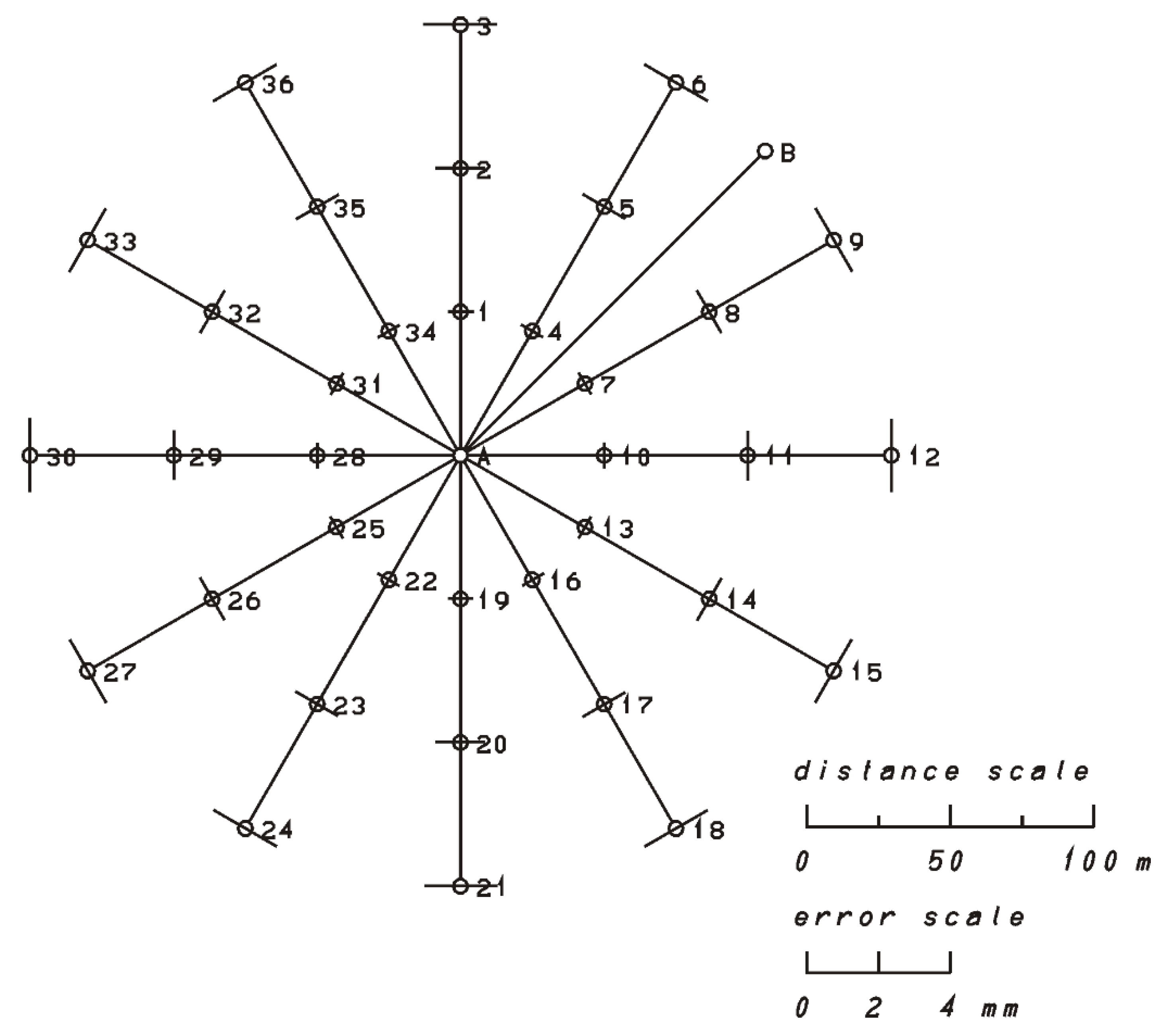
3.1. The Influence of the Temperature Displacements at Orientation Point $B$ on the Position of Control Point $C$

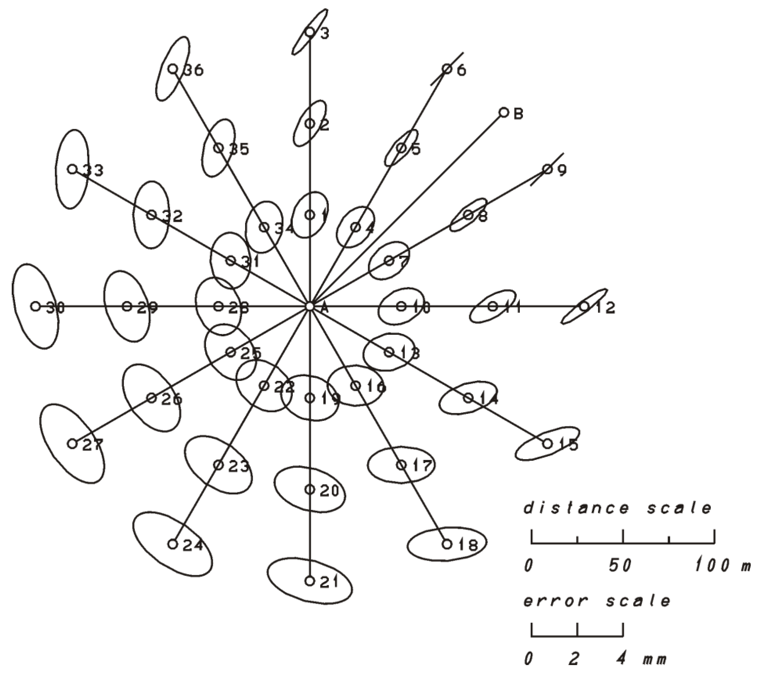
We will evaluate the precision of the coordinates of point $C$ for various coordinate differences $\mathsf{\Delta }{y}_A^C$ and $\mathsf{\Delta }{x}_A^C$ between points $A$ and $C$ using Equations (27)–(29). We used the variances ${\sigma }_{y_C}^2$ and ${\sigma }_{x_C}^2$ and the covariance ${\sigma }_{x{y}_C}$ to calculate the standard error ellipses (31), (33), and (35). Figure 7 and

Table 1. The precision of the position of the control point $C$ and the elements of the standard error ellipse due to the influence of the displacement as a result of the temperature difference at orientation point $B$.

${\nu }_{\mathit{A}}^{\mathit{C}}\left[\text{°}\right]$	${\mathit{d}}_{\mathit{A}\mathit{C}}\left[\mathbf{m}\right]$	${\mathit{\sigma }}_{\mathit{x}{\mathit{y}}_{\mathit{C}}}\left[{\mathbf{mm}}^2\right]$	${\mathit{\sigma }}_{{\mathit{y}}_{\mathit{C}}}\left[\mathbf{mm}\right]$	${\mathit{\sigma }}_{{\mathit{x}}_{\mathit{C}}}\left[\mathbf{mm}\right]$	$\mathit{a}$ [mm]	$\mathit{b}$ [mm]	$\mathit{\theta }$ [°]
0	50	0.00	0.33	0.00	0.33	0.00	90.00
0	100	0.00	0.67	0.00	0.67	0.00	90.00
0	150	0.00	1.00	0.00	1.00	0.00	90.00
30	50	0.05	0.29	0.17	0.33	0.00	120.00
30	100	0.19	0.58	0.33	0.67	0.00	120.00
30	150	0.43	0.87	0.50	1.00	0.00	120.00
60	50	0.05	0.17	0.29	0.33	0.00	150.00
60	100	0.19	0.33	0.58	0.67	0.00	150.00
60	150	0.43	0.50	0.87	1.00	0.00	150.00
90	50	0.00	0.00	0.33	0.33	0.00	180.00
90	100	0.00	0.00	0.67	0.67	0.00	180.00
90	150	0.00	0.00	1.00	1.00	0.00	180.00

show the direction and shape of the standard error ellipses resulting from the displacement of the orientation point $B$ for different positions of the control point $C$. We have shown ellipses for different positions of the simulated points, different bearings between points $A$ and $C$ (${\nu }_A^C=0°,30°,60°,90°,120°,150°,180°,210°,240°,270°,300°,330°$) and different distances between the points ($d_{AC}=50,100,150\mathrm{m}$) and for various coordinate differences between points $A$ and $C$. The bearing between survey point $A$ and the orientation point $B$ is ${\nu }_A^B=45°$, while the distance between survey point $A$ and orientation point $B$ is measured at $d_{AB}=150\mathrm{m}$.

Table 1 shows the precision of the position of the control point $C$ and the elements of the standard error ellipse due to the influence of the displacement of the orientation point $B$ for ${\sigma }_{y_B}^2={\sigma }_{x_B}^2=1{\mathrm{mm}}^2$ and ${\sigma }_{y{x}_B}=0{\mathrm{mm}}^2$ at different angles and distances between survey point $A$ and control point $C$ and ${\nu }_A^B=45°$, $d_{AB}=150\mathrm{m}$.

From Figure 7 and the values in Table 1, we can see that:

• we have the limit case of the error ellipses with one principal axis equal to zero,
• the direction of the major semi-axis is orthogonal to the line connecting points $A$ and $C$,
• the semi-major axis increases with the distance from the control point $C$.

The displacements of the orientation point $B$ therefore not only causes an error in the measuring direction between survey point $A$ and orientation point $B$, but also lead to errors in the horizontal angle with the tip in survey point $A$ and branches in the direction of orientation point $B$ and control point $C$.

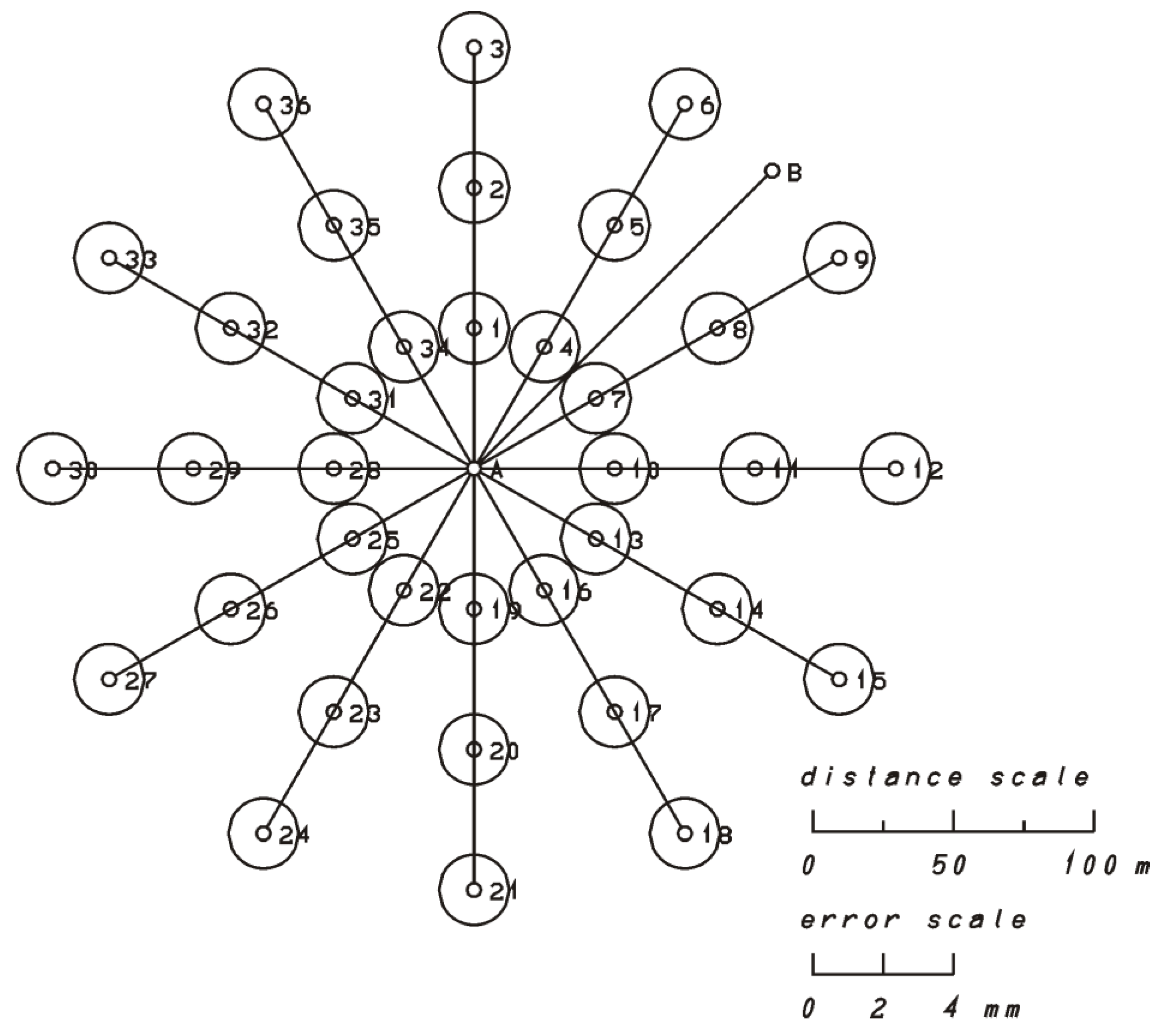
3.2. The Influence of the Temperature Displacements at Control Point $C$ on the Position of Control Point $C$

If the control point $C$ has been displaced due to the temperature load on the pillar, the error ellipses are of course the same regardless of the angles of orientation and the distances between the points, which is clearly shown in Figure 8.

3.3. The Influence of the Temperature Displacements at Survey Point $A$ on the Position of the Control Point $C$

With Equations (49)–(51), we have expressed the precision of the control point $C$ for the orientation angle 45° between the survey point $A$ and the orientation point $B$ and a distance of 150 m, as well as for different bearings (0°, 30°, 60°, 90°, 120°, 150°, 180°, 210°, 240°, 270°, 300°, 330°) and distances (50, 100, and 150 m) between survey point $A$ and control point $C$. Figure 9 and

Table 2. The precision of the position of the control point $C$ and the elements of the standard error ellipse due to the temperature displacements at the survey point $A$.

${\nu }_{\mathit{A}}^{\mathit{C}}\left[\text{°}\right]$	${\mathit{d}}_{\mathit{A}\mathit{C}}\left[\mathbf{m}\right]$	${\mathit{\sigma }}_{\mathit{x}{\mathit{y}}_{\mathit{C}}}\left[{\mathbf{mm}}^2\right]$	${\mathit{\sigma }}_{{\mathit{y}}_{\mathit{C}}}\left[\mathbf{mm}\right]$	${\mathit{\sigma }}_{{\mathit{x}}_{\mathit{C}}}\left[\mathbf{mm}\right]$	${\mathit{\sigma }}_{\mathit{C}}\left[\mathbf{mm}\right]$	$\mathit{a}$ [mm]	$\mathit{b}$ [mm]	$\mathit{\theta }$ [°]
0	50	0.24	0.80	1.00	1.28	1.06	0.72	26.30
0	100	0.47	0.71	1.00	1.23	1.13	0.47	31.07
0	150	0.71	0.77	1.00	1.26	1.24	0.24	36.84
30	50	0.27	0.82	0.89	1.21	1.01	0.67	38.97
30	100	0.45	0.72	0.80	1.08	1.02	0.35	41.13
30	150	0.53	0.72	0.74	1.03	1.03	0.03	44.53
60	50	0.27	0.89	0.82	1.21	1.01	0.67	51.03
60	100	0.45	0.80	0.72	1.08	1.02	0.35	48.87
60	150	0.53	0.74	0.72	1.03	1.03	0.03	45.47
90	50	0.24	1.00	0.80	1.28	1.06	0.72	63.70
90	100	0.47	1.00	0.71	1.23	1.13	0.47	58.93
90	150	0.71	1.00	0.77	1.26	1.24	0.24	53.16
120	50	0.13	1.12	0.82	1.39	1.14	0.80	77.72
120	100	0.36	1.26	0.72	1.45	1.30	0.64	72.79
120	150	0.69	1.40	0.72	1.58	1.50	0.50	67.99
150	50	−0.04	1.22	0.89	1.51	1.22	0.89	93.11
150	100	0.02	1.47	0.80	1.67	1.47	0.80	89.24
150	150	0.17	1.72	0.74	1.88	1.73	0.73	85.92
180	50	−0.24	1.26	1.00	1.61	1.29	0.96	109.49
180	100	−0.47	1.55	1.00	1.84	1.59	0.92	107.10
180	150	−0.71	1.85	1.00	2.10	1.90	0.90	105.18
210	50	−0.37	1.22	1.12	1.66	1.33	1.00	126.44
210	100	−0.84	1.47	1.26	1.93	1.66	0.99	125.63
210	150	−1.40	1.72	1.40	2.22	1.99	0.99	125.01
240	50	−0.37	1.12	1.22	1.66	1.33	1.00	143.56
240	100	−0.84	1.26	1.47	1.93	1.66	0.99	144.37
240	150	−1.40	1.40	1.72	2.22	1.99	0.99	144.99
270	50	−0.24	1.00	1.26	1.61	1.29	0.96	160.51
270	100	−0.47	1.00	1.55	1.84	1.59	0.92	162.90
270	150	−0.71	1.00	1.85	2.10	1.90	0.90	164.82
300	50	−0.04	0.89	1.22	1.51	1.22	0.89	176.89
300	100	0.02	0.80	1.47	1.67	1.47	0.80	0.76
300	150	0.17	0.74	1.72	1.88	1.73	0.73	4.08
330	50	0.13	0.82	1.12	1.39	1.14	0.80	12.28
330	100	0.36	0.72	1.26	1.45	1.30	0.64	17.21
330	150	0.69	0.72	1.40	1.58	1.50	0.50	22.01

show the direction and shape of the standard error ellipses (52), (53), and (54), which occur as a result of the temperature displacements at the survey point $A$ for various positions of the control point $C$.

Table 2 shows the influence of the temperature displacements at survey point $A$ on the precision of the position of the control point $C$ and the elements of the standard error ellipses when ${\sigma }_{y_A}^2={\sigma }_{x_A}^2=1{\mathrm{mm}}^2$ and ${\sigma }_{y{x}_A}=0{\mathrm{mm}}^2$ at different angles and distances between survey point $A$ and control point $C$, ${\nu }_A^B=45°$, $d_{AB}=150\mathrm{m}$.

If we look at the influence of the temperature displacements at survey point $A$ on the position of control point $C$, Equations (52)–(54), in combination with the representations of the error ellipses in Figure 9 and the values in Table 2, we see that:

• the error ellipses increase with distance from the control point $C$,
• the major semi-axis of the error ellipses reaches a size of 2 mm, which is significant if we take into account the fact that for the survey point $A$ we assumed the variances to be ${\sigma }_{y_A}^2={\sigma }_{x_A}^2=1{\mathrm{mm}}^2$ and ${\sigma }_{y{x}_A}=0{\mathrm{mm}}^2$,
• that the standard deviation of the distance between measured and exact position of the control point ${\sigma }_C=\sqrt{{\sigma }_{y_C}^2+{\sigma }_{x_C}^2}$ exceeds the value of 2.2 mm, which is significant in precise measurements,
• with increasing distance between survey point $A$ and orientation point $B$, the influence of the horizontal angle error on the precision of control point $C$ decreases and the distance error becomes more and more influential.

The displacement of survey point $A$ thus influences all measurements, i.e., the measured horizontal direction to points $B$ and $C$, and the distance between survey point $A$ and control point $C$.

The error of determining the position of the control point $C$ has a considerable influence on the error of the measured direction from survey point $A$ to control point $C$ and consequently on the horizontal angle with its apex at survey point $A$ and the intersections in the direction of orientation point $B$ and control point $C$ as well as the measured distance between survey point $A$ and control point $C$.

4. Conclusions

If we want to determine the displacements of the control points located on the object, we need well stabilized reference points, which must be in the same position during the individual measurements. Since the points are usually stabilized in nature, they are constantly exposed to changing natural conditions. Apart from different movements of the ground, the positions of these points, when stabilized by measuring pillars, can be influenced by temperature loads due to solar radiation. These loads lead to a deflection of the measuring pillar, which moves the screw for forced centering, which is attached to the top of the pillar and to which we attach the tachymeter or prism. If we use such a pillar or point for measuring, our measurements may show an error in distance or horizontal direction due to the deflection of the pillar.

Control measurements show whether the object has been displaced. Due to temperature related deflections of the pillar, which can lead to considerable measurement errors, we may come to a wrong conclusion. We could conclude that the displacement of the object did not take place although it did, or we could come to the opposite conclusion and find that a displacement took place although the object remained still.

In this paper, we have shown that if such a displacement occurs at the orientation point, it can be minimized with a sufficient distance between the survey and orientation points. If such a displacement occurs at the survey or control point, it cannot be eliminated by geometrically dividing the points. However, we can try to minimize its effect by measuring under conditions that do not lead to a temperature variation in the pillar body and temperature induced displacements.

References

- Grigillo, D.; Stopar, B. Methods of gross error detection in geodetic observations. Geod Vestn 2003, 47, 387–403. Available online: http://www.geodetski-vestnik.com/47/4/gv47-4_387-403.pdf (accessed on 3 November 2020).
- Močnik, R.; Koler, B.; Zupan, D.; Ambrožič, T. Investigation of the Precision in Geodetic Reference-Point Positioning Because of Temperature-Induced Pillar Deflections. Sensors 2019, 19, 3489. [Google Scholar] [CrossRef] [PubMed]
- Močnik, R. Temperature Effect Analysis of Reinforced Concrete Observation Columns. Master’s Thesis, Faculty of Civil and Geodetic Engineering, University of Ljubljana, Ljubljana, Slovenia, 2016. [Google Scholar]
- Kahmen, H.; Faig, W. Surveying, 1st ed.; Walter de Gruyter: Berlin, Germany, 1988. [Google Scholar]
- García-Balboa, J.L.; Ruiz-Armenteros, A.M.; Rodríguez-Avi, J.; Reinoso-Gordo, J.F.; Robledillo-Román, J. A Field Procedure for the Assessment of the Centring Uncertainty of Geodetic and Surveying Instruments. Sensors 2018, 18, 3187. [Google Scholar] [CrossRef] [PubMed]
- Ghilani, C.D.; Wolf, P.R. Adjustment Computations: Spatial Data Analysis, 4th ed.; John Wiley & Sons: Hoboken, NJ, USA, 2006. [Google Scholar]
- Baykal, O.; Tari, E.; Coskun, M.Z.; Erden, T. Accuracy of Point Layout with Polar Coordinates. J. Surv. Eng.-ASCE 2005, 131, 87–93. [Google Scholar] [CrossRef]
- Lambrou, E.; Nikolitsas, K. Detecting the Centring Error of Geodetic Instruments Over a Ground Mark Through a Tribrach-based Optical Plummet. Appl. Geomat. 2017, 9, 237–245. [Google Scholar] [CrossRef]
- Schofield, W. Engineering Surveying: Theory and Examination Problems for Students, 4th ed.; Butterworth-Heinemann: Oxford, UK, 1998. [Google Scholar]
- Ruiz-Armenteros, A.M.; García-Balboa, J.L.; Mesa-Mingorance, J.L.; Ruiz-Lendínez, J.J.; Ramos-Galán, M.I. Contribution of Instrument Centring to the Uncertainty of a Horizontal Angle. Surv. Rev. 2013, 45, 305–314. [Google Scholar] [CrossRef]
- Leick, A. Adjustment Computation; Department of Spatial Information Science and Engineering, University of Main: Orono, MA, USA, 1980. [Google Scholar]
- Jӓger, R.; Müller, T.; Saler, H. Klassische und Robuste Ausgleichungverfahren: Ein Leitfaden für Ausbildung und Praxis von Geodäten und Geoinformatikern; Herman Wichmann Verlag: Heidelberg, Germany, 2005. [Google Scholar]
- Leick, A.; Humpehrey, D. Adjustment with Examples; Department of Spatial Information Science and Engineering, University of Main: Orono, MA, USA, 1986. [Google Scholar]