Article

A Posteriori Detection of Numerical Locking in hpq-Adaptive Finite Element Analysis

by
Łukasz Miazio
1 and
Grzegorz Zboiński
1,2,*
1
Faculty of Technical Sciences, The University of Warmia and Mazury, Oczapowskiego 11, 10-719 Olsztyn, Poland
2
Institute of Fluid Flow Machinery, Polish Academy of Sciences, Fiszera 14, 80-231 Gdańsk, Poland
*
Author to whom correspondence should be addressed.
Appl. Sci. 2020, 10(22), 8247; https://doi.org/10.3390/app10228247
Submission received: 29 September 2020 / Revised: 13 November 2020 / Accepted: 17 November 2020 / Published: 20 November 2020

Abstract

:
The proposed detection algorithms are assigned for the h p q -adaptive finite element analysis of the solid mechanics problems affected by the locking phenomena. The algorithms are combined with the M- and h p q -adaptive finite element method, where M is the element model, h denotes the element size parameter, and p and q stand for the longitudinal and transverse approximation orders within an element. The applied adaptive scheme is extended with the additional step where the locking phenomena are a posteriori detected, assessed and resolved. The detection can be applied to shear, membrane, or shear–membrane locking phenomena. The removal of the undesired influence of the numerical locking on the problem solution is based on p-enrichment of the mesh. The detection algorithm is also enriched with the locking assessment algorithm which is capable of determination of the optimized value of p which is sufficient for the phenomena removal. The detection and assessment algorithms are based on a simple sensitivity analysis performed locally for the finite elements of the thin-walled domain. The sensitivity analysis lies in comparison of the element solutions corresponding to two values of the order p, namely current and potentially eliminating the locking. The local solutions are obtained from the element residual method. The elaborated algorithms are original, relatively simple, extremely reliable, and highly effective.

1. Introduction

This paper concerns application of the algorithms for detection, assessment and resolution of numerical locking in the h p q -adaptive finite element elastic analysis of thin-walled structures or complex structures which include thin-walled, solid, and transition parts. We consider all cases when the influence of the locking phenomenon on the problem solution is significant. We focus on the theoretical and methodological aspects such as the idea and justification of the elaborated algorithms for a posteriori detection and assessment of the phenomenon. In addition, the necessary modification of the applied h p q -adaptive algorithms is of our interest. The employed model- and h p q -adaptive method allows for different element size h, different element longitudinal and transverse orders of approximation, p and q, and different element model M in each finite element. The paper also presents application of the introduced detection, assessment, and resolution algorithms in the h p q -adaptive analysis of structural elements. These algorithms are investigated in the contexts of their generality, reliability, and effectiveness.

1.1. State-of-the-Art Issues

We address two specific issues dealt with the locking phenomena. The first one concerns some basic research on the nature of this phenomenon, while the second issue is the existing methods of removal of the numerical consequences of the phenomenon.

1.1.1. Theoretical and Numerical Research of Locking Phenomena

The numerical locking phenomena concern thin-walled structures in which the true solution is characterized by bending strains dominance over shear and/or membrane strains. The phenomenon does not appear in the case of the membrane strains dominance. If, due to poor discretization of the problem, the shear and/or membrane strains are not equal to zero, as it results from the thin-walled theories for the thickness t tending to 0, then the shear, membrane, or shear–membrane strain energy numerically dominates over the bending energy, leading to numerical over-stiffening of the structure, which in turn results in too low (zero or almost zero) values of displacements (compare the work [1]). This phenomenon is called the shear, membrane, or shear–membrane locking and is typical for the displacement finite element method.
Theoretical and numerical studies of the locking phenomena concern one- and two-dimensional problems, including beams, arcs, plates, and shells. Different kinds of locking are investigated: volume (Poisson’s) locking present in nearly incompressible materials ( ν 0.5 ), deformational locking present in bending-dominated thin-walled structures within the displacement formulation of the finite element method, and finally the trapezoidal locking present in hybrid-stress finite elements. The deformational locking, which is the subject of this work, may be shear (plates), membrane, or shear–membrane (shells). The significant exemplary theoretical and numerical research results concerning deformational locking are presented in [1,2,3,4,5,6], respectively. These works refer to the first-order, higher-order, and hierarchical models of plates and shells.

1.1.2. Overcoming the Locking Phenomena

We limit this survey to the methods related to the shear and/or membrane locking. This type of locking results from the thick- or thin-walled character of the plate and shell structures.
The first method of overcoming the locking is based on application of the mixed or hybrid formulations of the finite element method instead of the displacement formulation. This leads to elements of the class C 1 instead of the class C 0 . The elements of this group are usually of low-order and may need stabilization. The examples of the elements of this group are presented in [7,8,9]. More recent examples of the mixed and hybrid finite elements resistant to locking are published in [10,11].
The second approach takes advantage of the so-called reduced or reduced selective numerical integration, sometimes enriched with the stabilization matrix which removes deformation modes of zero energy. The reduced integration consists in integration of the stiffness matrix with the numerical integration parameters as for the elements described with the polynomial interpolation of one order lower. In the selective version of the reduced integration the lower order is applied to a part of the stiffness matrix, responsible for the locking, i.e., the part corresponding to shear and/or membrane strain energy. The examples of application of this approach to plate and shell elements can be found in [12,13,14]. The recent works dealing with the reduced and reduced selective integration concern either the isogeometric analysis or the standard finite element methods, for example, in [15,16].
The third way to overcome the phenomenon lies in introduction of the discrete Kirchhoff constraints into the elements of the class C 0 . The method is directed towards removal of the shear locking and requires that the Kirchhoff constraints are imposed on the selected points or lines within C 0 element. The prominent examples of plate or thick shell elements of this type can be found in [17,18]. Recent examples of the discrete Kirchhoff and Kirchhoff-Love constraints are presented in the works [19,20].
The fourth method consists in application of the consistent (interdependent) fields of the transverse displacement and rotations, one order higher in the case of the mentioned displacement. The method leads to different numbers of unknowns of both types within an element. The surplus displacement degrees of freedom (dofs) are removed from the model based on the condition of zero transverse shear strains and/or zero membrane strain condition. The prominent examples of this method of the locking removal can be found in [21,22].
The fifth approach is based on the assumed shear or membrane strains consistent with the interpolated transverse displacement at some points. In this method, bending strains result from the interpolated displacement field, while the transverse shear and/or membrane (in-plane) strains possess the assumed form resulting from the interpolation based on some chosen points. The significant works, leading to the current state of this method in relation to quadrilateral plate and shell elements, are found in [23,24,25]. Two versions of the presented approach, based on either the enhanced assumed strains or assumed natural strains, are still being developed, for example, in [26,27].
The sixth method lies in application of higher-order elements conforming to the displacement finite element formulation. The examples of application of such elements in the case of the classical (non-adaptive) finite element methods, can be found in [28,29]. In the non-adaptive methods, plate or shell elements conforming to the first-order or higher-order theories are applied. The fixed longitudinal order of h-approximation up to the fifth order is usually applied within elements of this type. The adaptive quadrilateral elements, conforming to hierarchical approximations and higher-order shell models, are used in [30]. The hexahedral elements corresponding to three-dimensional elasticity, equipped with independent transverse and longitudinal approximations of the higher order, and assigned for plate and shell analysis, are proposed in [31] and applied in h p -adaptive version in [32], for example. The recent applications of the higher-order models and approximations to locking removal are presented in the works [33,34]. These proposals are not consistent with the hierarchical approach.
Let us conclude the above survey of the methods of overcoming the locking phenomena in the context of needs of the h p q -adaptive method for complex structures analysis. Firstly, it should be noticed that only low-order longitudinal approximations and first-order plate and shell models are possible in the cases of the mixed and hybrid methods, the uniform or selective reduced integration, and the consistent field method. In the case of the discrete Kirchhoff constraints, only shear locking can be removed effectively. Additionally, this method of removal leads to large variability of elements. In the case of the assumed strains approach, the claimed generalization of the method for high-order in-plane approximations has not been proved in practice. For the reduced integration and assumed stress method, there are problems with their application to triangular or prismatic elements. In the case of the discrete Kirchhoff constraint and consistent field methods of removal, one deals with different number and location of translational and rotational degrees of freedom. Note that the higher-order elements are free from all these defects. Due to our earlier choices concerning the applied hierarchical models and h p q -approximations, the displacement formulation of such elements becomes our obvious choice.

1.1.3. Detection and Assessment of the Locking

The basic method of detection and assessment of the locking phenomena is the a priori theoretical analysis of the numerical solutions of the model problems potentially suspected to be a subject of locking (see Section 1.1.1 of this literature survey). Another interesting method of detection and assessment of the locking in the one- and two-dimensional elements is proposed in [35,36]. It is based on application of the finite difference operators corresponding to the problem local formulation. In [37,38,39], the numerical methods of detection and assessment of the phenomenon are proposed. These methods are based on the sensitivity analysis, i.e., two or a sequence of local problems are solved for each element of the potentially affected domain.

1.2. The Applied Methodology

Two issues are addressed here. The first one deals with the best choice of the method of effective detection and assessment of the locking phenomena. The second issue is related to the numerical methods of removing the phenomena.
It results from the above literature survey that the available knowledge on the locking phenomena allows understanding of the nature and sources of appearance of the phenomena. The accumulated knowledge on the phenomenon allows also for a priori determination of the solution convergence of the problems where the phenomena appear. The main difficulty in the direct application of these results in the numerical analysis of any arbitrary thin-walled structure is that the available results concern the specific model problems which may differ to the arbitrary problem under consideration.
The second conclusion from the literature survey is that the most effective way of removing the locking phenomena lies in application of the higher-order longitudinal p-approximation of the displacement field in the analyzed thin-walled structure or a thin-walled part of the complex structure.
It also results from the literature that some detection methods of the phenomena exist. Among these methods, the approach proposed in [37,38,39] seems to be best suited for adaptive analysis. This approach is based on the same numerical techniques that are applied in the error-controlled adaptivity.
The main feature of the proposed a posteriori detection, assessment and removal of the locking phenomena is that the adaptation process requires four steps, instead of the standard three steps of the error-controlled h p -adaptivity proposed in [40]. The additional step of adaptation, which lies in initial mesh modification, incorporates not only the automatic removal of the locking phenomena but also the automatic resolution of the boundary layers [38]. The main idea standing behind the additional adaptation step is to move the numerical solution, obtained with use of h p -approximations [41,42], to the asymptotic convergence range. Within this range, the standard h- and p-adaptation steps can be made based on the h p -convergence theorem and upper-bounding values of the global error estimates from the equilibrated residual method [43,44].
Finally, it should be noted that our detection and assessment tools are based on sensitivity analysis, not on the estimated error values themselves. Thanks to this, requirements concerning the error estimation can be relaxed.

1.3. Novelty of the Paper

The novelty of this work consists in the new algorithms for a posteriori detection and assessment of the numerical locking phenomena. This refers to shear, membrane, or shear–membrane locking. With these new algorithms, one is able to detect the presence of the phenomenon and assess its strength so that the adequate numerical means can be used to remove the phenomenon. The proposed numerical means of the removal consist in introduction of the new adaptation step, called the modification one, into the existing three-step, model- and h p q -adaptive finite element procedure for analysis of complex structures. The new step employs the mentioned detection and assessment algorithms and performs modification of the initial mesh through p-enrichment. The numerical cost of this new step is low as the detection and assessment is performed on the initial, usually coarse mesh.
The applied adaptive method [38,45,46], the new algorithms are incorporated in, takes advantage of the hierarchical models proposed in [31,47], hierarchical h p -approximations elaborated in [41,42], a posteriori error estimation from [30,43,44], and error-controlled adaptive procedure given in [40].

2. Preliminaries

Two issues are addressed in this section. The first one deals with the model problems considered in this research. The second one is presentation of the nature of the locking phenomena.

2.1. Model Problems

Let us consider a wide range of problems of linear elasticity covered by the standard local (strong) formulation
σ , j i j + f i = 0 σ i j = D i j k l ε k l ε k l = 1 2 ( u k , l + u l , k ) , x V
composed of the equilibrium, constitutive, and geometrical equations, respectively. Above, i , j , k , l = 1 , 2 , 3 , while the smooth components f i L 2 ( V ) stand for the known body loading vector, with V representing volume of the body. The tensor components σ i j and ε k l stand for stresses and strains, while the unknown vector components u k denote displacements. The terms D i j k l are components of the fourth-order tensor of elasticities. The elasticities are symmetric D i j k l = D j i k l = D i j l k = D k l i j and satisfy the strong and uniform ellipticity condition: D i j k l ξ i j ξ k l α ξ i j ξ k l , ξ i j = ξ j i , where ξ i j is any real-valued tensor of the second rank and α is a positive constant. Note that such elasticities may correspond to three-dimensional stress and strain states or to the constrained, plane stress or plane strain, states. Note also that, for the specific case of isotropy, the elasticities can be expressed by the Young’s modulus E and Poisson’s ratio ν .
The set (1) has to be completed with the displacement and stress boundary conditions of the form
σ i j n j = p i , x S P u i = w i , x S W
where i , j = 1 , 2 , 3 , while the smooth components p i L 2 ( S ) and the terms w i stand for the known values of stress vector components and displacement vector components on the parts S P and S W of the surface S V of the body V, with S = S P S W and S P S W = . The vector components n j represent unit outward normal to the surface part S P = S T S B composed of the top S T and bottom S B surfaces of the body. The way they are determined is explained below.
Equation (1) is valid within the body volume V. Such a volume may represent thick- or thin-walled structures or complex structures containing such parts. Due to the model character of the considerations of this section, we limit ourselves to the first case. The corresponding thin-walled domain of the volume V is sufficiently smooth (Lipschitzian or smoother), open, and bounded region. As we apply the 3D Cartesian description of the problem, i.e., we employ Cartesian coordinates x, the following explicit (curvilinear) and implicit (Cartesian) definitions of the volume V are appropriate:
V = η R 3 : ( η 1 , η 2 ) S M , η 3 ( t / 2 , t / 2 ) x ( η ) R 3 : x = F ( η ) , ( η 1 , η 2 ) S M , η 3 ( t / 2 , t / 2 )
where F is the reversible map converting the curvilinear coordinates η into the Cartesian ones x. The function t = t ( η 1 , η 2 ) measures the symmetric thickness in the direction η 3 normal to the mid-surface S M . The mid-surface S M , where η 3 = 0 , of the thin-walled body can be any sufficiently smooth (Lipschitzian or smoother), two-dimensional, open and bounded region. Formal definition of the thin-walled body geometry also needs introduction of the lateral part S L of the body boundary S as well as the upper (top) S T and lower (bottom) S B parts of this boundary. More details on the applied definition of the thin-walled geometry can be found in [48].
The considered model problem, described by the local (strong) formulation (1), completed with the boundary conditions (2), can also be presented in the weak variational form:
B ( u , v ) = L ( v )
where the admissible displacement vector is v 𝒱 , while the corresponding space reads 𝒱 = { v ( H 1 ( V ) ) 3 : v = 0 o n S W } . The solution function for displacements is u w + 𝒱 , with w standing for the lift of the Dirichlet data (see [41]). This lift is consistent with the second equation (2). The bilinear form B ( v , u ) and linear form L ( v ) from the above functional represent the virtual strain energy and the virtual work of the external body and surface loadings, f and p, respectively, i.e.,
B ( u , v ) = V ε T ( v ) D ε ( u ) d V L ( v ) = V v T f d V + S P v T p d S
Above, D stands for the matrix representation of the elasticity constant tensor present in the second Equation (1), while ε is the six-component vectorial representation of the strain tensor defined with the third Equation (1).
Let us introduce now the finite element approximation of the variational functional (4). The approximation is based on the general rules of h p approximations [41], applied to 3D-based hierarchical shell models of order q presented in [38,45]. The approximated variational functional reads
B ( u h p q , v h p q ) = L ( v h p q )
where the approximated admissible displacements v h p q 𝒱 h p q belong to the space 𝒱 h p q = { v h p q ( H 1 ( V ) ) 3 : v h p q = 0 o n S W } . Additionally, u h p q w h p q + 𝒱 h p q , with the approximated values w h p q of the lift w.
Note that the approximated variational formulation (6) can also be expressed in the language of finite elements
K q h p q = F
where K and F are the global stiffness matrix and the global forces vector, while q h p q stands for the displacement dofs vector corresponding to the solution field u h p q of displacements.

2.2. Locking Phenomena

It was demonstrated in a numerous works (see [49,50], for example) that the three-dimensional elasticity description of the strain energy U 1 2 B ( u , u ) of the thin-walled body V tends to the following limit value when the thickness of the body tends to zero, t 0 :
U = 1 2 V σ i j ε i j d V 1 2 V [ σ α β ε α β + σ 33 ε 33 + 2 σ 3 β ε 3 β ] d V 1 2 t S M E 1 ν 2 [ ( 1 ν ) γ α β γ α β + ν γ α α γ β β ] d S M + 1 2 t S M E k 1 + ν ( γ α 3 γ α 3 + γ 3 β γ 3 β ) d S M + 1 2 t 3 S M E 12 ( 1 ν 2 ) [ ( 1 ν ) κ α β κ α β + ν κ α α κ β β ] d S M = U m + U s + U b
Above, the three-dimensional components of the stress and strain tensors, σ i j and ε i j , i , j = 1 , 2 , 3 , of the three-dimensional theory of elasticity can be expressed in the thin limit with the two-dimensional longitudinal strain components of the mid-surface S M , γ α β , α , β = 1 , 2 ; transverse strain components, γ α 3 and γ 3 β , α , β = 1 , 2 ; and the components of the tensor of curvature variation, κ α β , α , β = 1 , 2 . Additionally, in the thin limit, the three-dimensional isotropic elasticity constants can be replaced with the isotropic plane stress constants of the first-order shell theory, expressed by the Young’s modulus E and the Poisson’s ratio ν and resulting from the plane stress assumption σ 33 = 0 . In addition, the kinematic condition of no elongation of the normals to the mid-surface, γ 33 = 0 , comes into play. The thin limit strain energy can then be approximated with the limit values of the membrane, shear, and bending parts, U m , U s , U b , of the strain energy U. The quantity k is the shear strain correction factor, equal to 5 / 6 and resulting from the applied first-order model which leads to false (constant) transverse-shear stresses.
Depending on the geometry, loading and kinematic boundary conditions, one may distinguish between the bending-dominated problems, when
U b U m + U s
and membrane-dominated or shear–membrane-dominated problems, where
U m U b , U s 0 U m + U s U b
respectively. Then, it results from (9) that, in the analytical solution of the bending-dominated problems, the shear and membrane strains should be equal or very close to zero, i.e.,
γ 13 = γ 31 0 , γ 23 = γ 32 0
for the plate and shell structures, and
γ 11 0 , γ 12 0 , γ 22 0
for the shell structures where the coupling of the membrane and bending strains exists. Note that the decoupling of the membrane and bending strains shown by the limit expression of the relation (8) exists only in the thin limit ( t 0 ) for the first-order shells, while for the first-order plates it holds for any thickness t.
The shear and shear–membrane lockings are purely numerical phenomena which happen for poor discretizations and result from insufficiently accurate approximation of the analytical constraints (11) and/or (12). If such inaccurate approximation occurs then the shear and/or membrane strains are too large and the shear and membrane strain energies grow. These energies dominate over the bending strain energy, leading to numerical over-stiffening of the structure, which in turn gives too small (locked) values of displacements of the numerical solution. Remembering that U h p q 1 2 B ( u h p q , u h p q ) 1 2 ( q h p q ) T K q h p q , one has
K q h p q = F , F I = const , K I J q J h p q
where K I J , F I are components of the global stiffness matrix and the global forces vector, with I , J = 1 , 2 , , N and N being the global number of degrees of freedom (dofs). The components q J h p q represent the global vector of unknown displacement dofs q h p q corresponding to the approximated field of displacements u h p q .

3. Locking Detection, Assessment, and Resolution

The proposed ideas of locking detection, assessment, and resolution are based on application of three existing numerical techniques. The first one is the equilibrated residual method of error estimation [43,44], here applied to solution of the local problems of two types. The second idea is sensitivity analysis based on comparison of the solutions to two local problems which differ with the longitudinal orders of approximation. The results of such a comparison can be used for the locking detection or assessment. If the locking is detected, then the mesh can be modified through the increase of the longitudinal order of approximation, by means of the standard p-enrichment technique [41,42].
The mentioned three techniques can be combined with the three-step h p -adaptive procedure controlled by the approximation error [51,52] or the automatic, iterative h p -adaptation driven by the interpolation error [41,42,53].

3.1. The Idea and Algorithm of a Posteriori Phenomenon Detection

The idea of a posteriori detection of the numerical locking was originally proposed by Zboiński [38]. Here, we develop and verify this idea. It consists in solution of two local problems for each element of the thick- or thin-walled part of the structure. The solutions to these problems are obtained from the equilibrated residual method. These two problems differ with the longitudinal order of approximation p. In the first problem, it is equal to its current value from the global problem under consideration. In the second local problem, its value corresponds to the problem potentially free of locking. For two mentioned solutions, the strain energy norms are calculated and compared. This corresponds to sensitivity analysis where the sensitivity of the solutions of the local problems to the change of the longitudinal order of approximation is assessed. Once the locking is detected, one may modify the mesh by increasing the current order of the longitudinal approximation to its value corresponding to the problems free of locking. The similar approach is used also for determination of the optimized value of the longitudinal approximation order which corresponds to the minimum value sufficient for removal of the phenomenon.

3.1.1. Solutions from the Equilibrated Residual Method

Let us recall now the equilibrated residual method of a posteriori error estimation, invented by Ainsworth and Oden [43]. All relations of this section are taken from the cited work. Here, we apply this method to the estimation of the numerical solutions of the 3D-based hierarchical shell problems [46]. The principal relation of the method is [44]
B ( e , v ) = B ( u H P Q u h p q , v ) = B ( u H P Q , v ) B ( u h p q , v ) = L ( v ) B ( u h p q , v ) , v 𝒱 H P Q ( V )
Above, u H P Q stands for either the exact solution of the problem or sufficiently accurate approximation of such a solution. The quantity e is the error vector corresponding to the assessed numerical solution u h p q . The kinematically admissible displacements v v H P Q belong to the space 𝒱 H P Q defined in analogy to the spaces introduced for (4) and (6). The discretization parameters H, P, and Q are the counterparts of h, p, and q from the relation (6). In the case of the exact solution ( u H P Q u ), one deals with 1 / H , P , Q , while in the case of the approximation, one deals with the finite values of the discretization parameters H, P and Q.
After noticing that e = u H P Q u h p q and introduction of this definition into the error functional (14), the latter simplifies to:
B ( u H P Q , v ) = L ( v ) , v 𝒱 H P Q ( V )
This way one searches for the approximation of the exact solution (displacements) of the problem instead of the problem error itself. However, once the displacements are determined, the error can be calculated from the above error definition. The presented approach is applied in the works [30,46], for example.
Let us now follow the work [43] and divide the domain V into E subdomains V e , corresponding to finite elements e = 1 , 2 , , E . The global functional (15) and its left- and right-hand side components can now be presented as a sum of the element contributions:
B ( u H P Q , v ) = e = 1 E B e ( u H P Q e , v e ) L ( v ) = e = 1 E L e ( v e ) = e = 1 E L e ( v e ) e = 1 E β e ( v e ) = e = 1 E L e ( v e ) + S e ( S P S W ) v T e r e ( u h p q ) d S e
where the element admissible displacements are defined as the global admissible displacements projected onto elements V e : v e v | V e . As demonstrated by Ainsworth and Oden [43], the sum of the auxiliary element functionals β e ( v e ) is equal to 0, as the internal load consistency condition must hold.
Above, the vectors r e ( u h p q ) represent the interelement loading due to equilibrated stresses. These stresses are defined in [43,44], for example. Their definition is as follows
r e ( u h p q ) = α f e r e ( u h p q ) + α e f r f ( u h p q )
where
r e ( u h p q ) = H ( ν e ) σ e ( u h p q ) , r f ( u h p q ) = H ( ν e ) σ f ( u h p q ) ,
and
H ( ν e ) = ν 1 0 0 ν 2 0 ν 3 0 ν 2 0 ν 1 ν 3 0 0 0 ν 3 0 ν 2 ν 1
The components of the unit normal vector ν e = [ ν 1 , ν 2 , ν 3 ] T are defined on the element surface S e . The vectorial six-component representations σ e and σ f of the stress tensors have to be determined for the element e and any of its neighbours f. The terms α f e and r e stand for the splitting function diagonal matrices and stress vectors. These matrices are: α f e = diag [ α 1 , α 2 , α 3 ] , with α f e = 1 α e f , 1 = diag [ 1 , 1 , 1 ] and directional components α m , m = 1 , 2 , 3 . The algorithms for calculation of the splitting functions in the case of the internally unconstrained and constrained (e.g., by the Reissner-Mindlin kinematic constraints) are described in [43,44,46], respectively. The alternative is replacement of the equilibrated stresses with their averaged counterparts: α f e = α e f = diag [ 1 2 , 1 2 , 1 2 ] .
Comparing relations (15) and (16) one can notice that the minimization of the global energy functional can be replaced with the minimization of local (element) functionals (see [43,44,46]). The element functionals read
u H P Q e 𝒱 H P Q e ( V e ) : B e ( u H P Q e , v e ) = L e ( v e ) + S e \ ( P Q ) v T e r e ( u h p q ) d S e , v e 𝒱 H P Q e ( V e )
where u H P Q e is the element solution function and 𝒱 H P Q e denotes the space of kinematically admissible element displacements v e v H P Q e . As shown in [43,44], the solution to the local problems (20) exists and is either unique or unique up to rigid body motions, for Dirichlet and Neumann boundary value problems, respectively. The mixed boundary value problems are also possible. Note that one deals with the Dirichlet problems for clamped elements adjacent to the external boundary of the structure, and with the Neumann problems for elements not adjacent to this boundary, namely for elements from the interior of the structure.

3.1.2. Check on Bending-Dominance of the Solution

Check on bending-dominance of the solution to the global problems of the type (6) was proposed by Zboiński [32]. Such a check is necessary as the locking phenomena are present only in the bending-dominated problems. In the membrane-dominated problems the phenomena do not appear. In addition, in the case of the mixed dominance, the locking may appear.

Strain Energy Components

In this work, we apply the proposed approach to the local solutions from the equilibrated residual method and to their sum. To apply this approach, one has to take into consideration that the strain energy approximation from (8) corresponds to the structures of the infinitely small thickness, for which the first-order theory can approximate the three-dimensional description. As we intend to check the locking phenomena in the structures of the finite thickness, described with the hierarchical models corresponding to higher-order shell theories, the decomposition of the three-dimensional strain energy into component energies typical for the first-order models can only be done approximately. Let us start with the following decomposition of the strain vector into its longitudinal, transverse and shear parts
ε = [ ε l , ε n , ε s ] T
where ε l = [ , ε α β , ] T , ε n = [ ε 33 ] T , ε s = [ , ε 3 α , ε α 3 , ] T and α , β = 1 , 2 are the local directions tangent to longitudinal directions of the thin-walled structure, and the index 3 corresponds to the local transverse direction. The analogous decomposition of the stress vector σ is also possible. Such decompositions lead to the division of the density υ of the total strain energy into the following components:
υ = σ i j ε i j = σ α β ε α β + σ 33 ε 33 + 2 σ 3 α ε 3 α = υ l + υ n + υ s
where i , j = 1 , 2 , 3 stand for the global Cartesian directions. In the above relation, the symmetries: σ 3 α = σ α 3 and ε 3 α = ε α 3 were taken into account. The terms υ l , υ n , υ s represent longitudinal, transverse, and shear components, respectively, of the density function. Consequently, the strain energy can also be divided into the corresponding energy components U l , U n , U s :
U = V υ d V = U l + U n + U s
Our calculations of the strain components of (21) on the element level correspond to the 3D-based hierarchical shell formulation proposed and developed in [38,45]. In this formulation local strains (defined in two longitudinal and the third transverse directions) and the global displacement dofs are applied. Because of that, the relation defining local strains ε (or their components) by the product of the element strain-displacement matrix B e (or its components) and the element displacement dofs vector q h p q e can be written as follows
ε = B e q h p q e = [ B l e , B n e , B s e ] T q h p q e = [ B l e q h p q e , B n e q h p q e , B s e q h p q e ] T = [ ε l , ε n , ε s ] T
where the longitudinal B l e , transverse B n e , and shear B s e blocks of the strain-displacement matrix include the latter matrix rows corresponding to the in-plane, normal and shear strain components: ε l , ε n , ε s . Note that the vector of displacement dofs is related to the displacement field u h p q e with the standard interpolation formula of the element e: u h p q e = N e q h p q e , where N e stands for the shape function matrix of the element.
Because of the 3D-based shell models applied in our research, further decomposition of the strain energy will be performed approximately. The exact decomposition is easy for the conventional shell models with the degrees of freedom defined on the mid-surface. Then, the dofs corresponding to the even and odd powers of the thickness contribute to the membrane and bending strains, respectively. In the 3D-based formulation, the dofs are defined along (or through) the thickness, and extracting their membrane and bending contributions needs much more complex procedure explained in [32]. The approximate procedure requires replacement of the top and bottom displacements of the symmetric thin-walled structure with their sums and differences which contribute to the mid-surface displacements and rotations. This allows for distinguishing the following components of the in-plane strains
ε α β γ α β + κ α β
where γ α β stand for the mid-surface strains (membrane strains) and κ α β are the three-dimensional counterparts of the change of curvature tensor (bending strains). With the above division, the in-plane density υ l of strain energy can be decomposed into three parts (membrane, bending, and coupling ones):
υ l υ m + υ b + υ c
that contain products of the membrane strains, bending strains, and their combination, respectively. Consequently, one also has
U l U m + U b + U c
Calculation of the two components of the right-hand side of (25) on the element level needs adequate transformation of the numerical representation of element longitudinal strains ε l , defined as a matrix product of the corresponding part of the strain-displacement matrix and the vector of displacement dofs. For the 3D-based hierarchical shell formulation, presented in [38,45], this transformation reads
ε l = B l e q h p q e = [ B t , B b , B o ] × [ q t , q b , q o ] T = [ B t + B b , B t B b , B o ] × [ 1 2 ( q t + q b ) , 1 2 ( q t q b ) , q o ] T = [ B s , B ϕ , B o ] × [ q s , q ϕ , q o ] T = B s q s + B ϕ q ϕ + B o q o = γ + κ + r γ + κ
where the sub-blocks B t , B b , and B o correspond to the top q t , bottom q b , and all other q o displacement dofs of the element dofs vector q h p q e . Location of the dofs of three types is on the top and bottom surfaces of the shell element, and apart from these two surfaces, respectively. In turn, the sub-blocks B s , B ϕ correspond to the mid-surface displacement dofs q s = 1 2 ( q t + q b ) and rotational dofs q ϕ = 1 2 ( q t q b ) . The approximate character of the performed transformation results from neglecting the mentioned other dofs in the resultant decomposition into the membrane and bending strain contributions.

The Criterion

In the criterion for detection of the dominance of bending strains, the solutions of two local problems from the equilibrated residual method are applied. The first solution corresponds to the following local discretization parameters: H = h , P 1 = p , and Q = q . In the second problem, set to be free of the locking phenomena, one has: H = h , P 2 = p m a x = 8 , and Q = q . The value of p m a x = 8 is taken from the research of Pitkaranta [4] who demonstrated that for such a value the membrane locking disappears in shell structures regardless of the thickness. For this value also the shear locking in plate structures disappears. It is well known that this type of locking is weaker than the membrane one in shells (compare remarks in [5,32], for example). The proposed criterion reads
e = 1 E U m e ( u H P 1 Q ) e + e = 1 E U s e ( u H P 1 Q ) e e = 1 E U b e ( u H P 1 Q ) e e = 1 E U m e ( u H P 2 Q ) e + e = 1 E U s e ( u H P 2 Q ) e < e = 1 E U b e ( u H P 2 Q ) e
The first condition detects dominance of the membrane and shear strains over the bending strains in the local problems corresponding to the global problem under consideration, while the second condition reflects the change of the dominance in the local problems. The form of the criterion corresponds to the shell structures, where coupling between shear, membrane and bending strains exists. In the case of plate structures, the coupling between the membrane strains and the shear and bending strains disappears and because of this the membrane strains have to be removed from the above criterion.
Fulfillment of the above criterion means that the true nature of the problem is bending-dominated and that the locking phenomenon appears in the assessed global problem. As a consequence, the locking has to be removed through increase of the approximation order p. The above criteria are necessary to confirm the results from the detection and assessment tools presented in the next sections, as those tools are not capable of distinguishing between the membrane- (and/or) shear-dominated problems and the bending-dominated ones.

3.1.3. Sensitivity Analysis of the Local Solutions

The main purpose of the sensitivity analysis performed in this section is detection of the situation that the assessed global problem solution differs to the solution of the problem potentially free of locking to such an extent that the difference may suggest the presence of the locking phenomena. Note that the theoretical ratio of the true bending-dominated solution and locked membrane-dominated (and/or shear-dominated) solution is C · t 2 , with C being a constant. This ratio results from the proportionality of the membrane (and/or shear) part of the strain energy and the bending part of this energy to t and t 3 , respectively, as shown in (8).
To compare the above two solutions, the following two local problems for each element of the plate or shell structure, or such parts of complex structures, has to be solved:
B e ( u H P 1 Q e , v H P 1 Q e ) L e ( v H P 1 Q e ) S e \ ( P W ) ( v H P 1 Q ) T e r e ( u h p q ) d S e = 0
where P 1 = p , H = h and Q = q correspond to the global problem under consideration, and:
B e ( u H P 2 Q e , v H P 2 Q e ) L e ( v H P 2 Q e ) S e \ ( P W ) ( v H P 2 Q ) T e r e ( u h p q ) d S e = 0
with P 2 = p m a x = 8 , H = h , and Q = q corresponding to the problem potentially free of locking.
The following criterion is set to assess sensitivity of the solution to the change of the longitudinal approximation order from P 1 to P 2 :
e = 1 E 1 2 B e ( u H P 1 Q e , u H P 1 Q e ) < a e = 1 E 1 2 B e ( u H P 2 Q e , u H P 2 Q e )
where a is the coefficient which determines the ability of the adaptive method to overcome the locking phenomena with the standard h p -adaptive procedure. In the case of the applied procedure based on Texas three-step strategy [40] and error estimation based on the equilibrated residual method [43,44], the reasonable (verified numerically) value is suggested to be equal to a = 0.1 . Fulfillment of the above criterion suggests the possibility of locking appearance. This possibility has to be confirmed by the criterion (29) of bending-dominance.

3.1.4. The Detection Algorithm

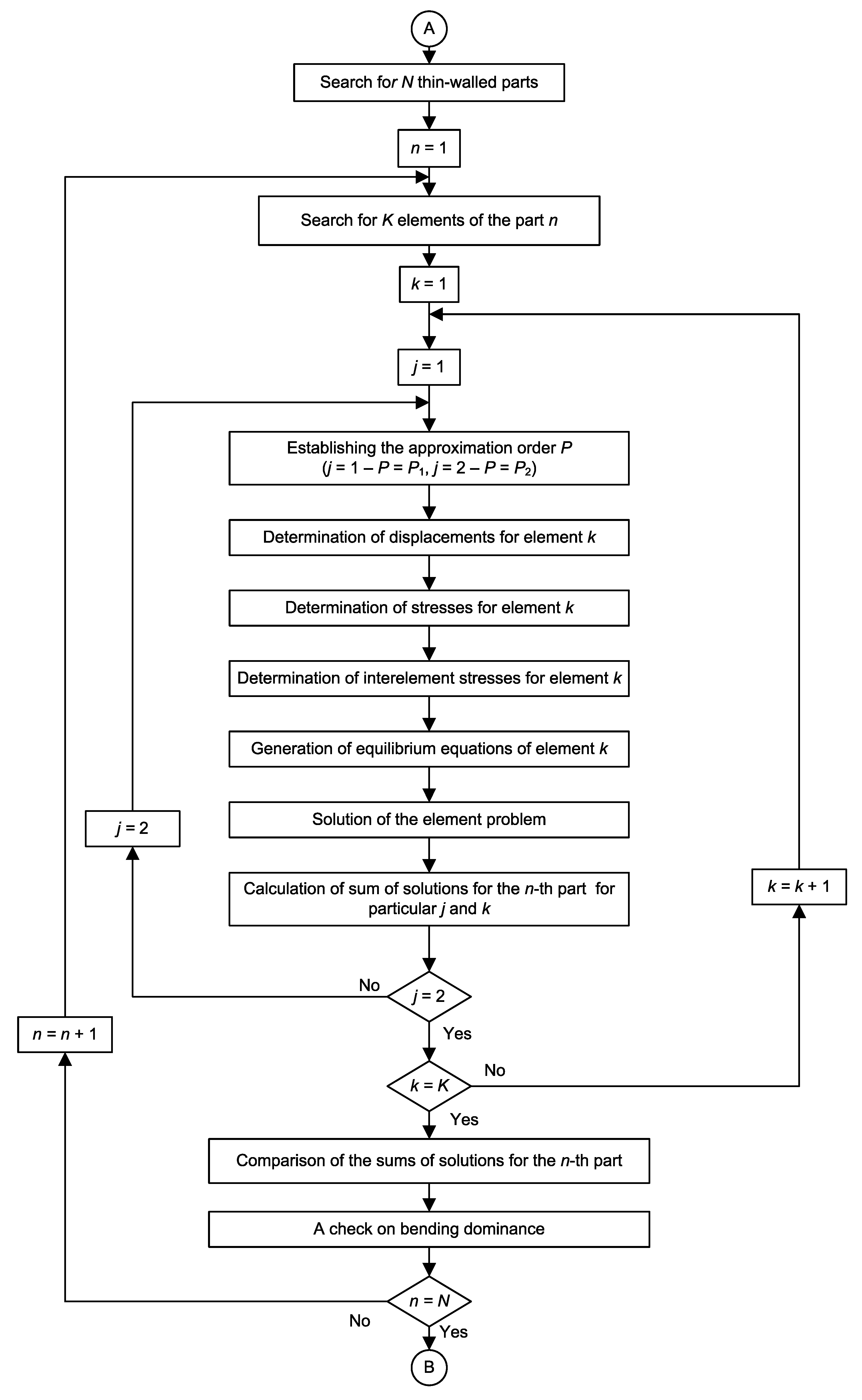
The algorithm of detection of the locking phenomena introduced into the standard three-step adaptive strategy proposed by Oden [40] is presented in Figure 1. The original part of the standard adaptation includes three steps: initial ( i = 1 ), intermediate ( i = 3 ) called also h-step, and final ( i = 4 ) called also the p-step. Either local h-refinement or local p-enrichment is performed within each element of the latter two steps, based on the estimated approximation error values obtained from the equilibrated residual method of Ainsworth and Oden [43,44]. The modification of the initial mesh ( i = 2 ) is performed as the second step when necessary. This additional step is composed of two stages: the detection of the phenomenon, and the changes in the mesh which consist in the global p-enrichment performed within all elements of the thin- or thick-walled structure or such a part of the complex structure.
The details of the additional step modifying the initial mesh are presented in Figure 2. At first, we search for the thick- or thin-walled parts of the generally complex structure. Such a structure can be composed of thick- and thin-walled parts, solid parts, and transition parts joining the previous two types of geometries. Of course, simple geometries composed of a single thin- or thick-walled part are also possible. Then, for each element of such a thin- or thick-walled part, the interelement stresses on the element boundary have to be calculated. Subsequently, for two local problems described with Equations (30) and (31), the terms of these equations are generated and the equations are solved. Next, one has to sum the element energies from (32) and compare two sums for two types of the local problems. Finally, if the criterion for locking detection is met, one has to confirm this result with the criterion for bending dominance detection (29). If it is fulfilled, then the modification of the initial mesh is performed, which is based on p-enrichment of all elements of the thin- or thick-walled part of the structure. Such elements of the modified structure are all equipped with the longitudinal order of approximation equal to p = p m a x = 8 . Next, the standard steps, i = 3 and i = 4 , of h p -adaptation can be performed.
It should be underlined that calculation of the interelement stresses, performed in the above algorithm, is skipped in this paper as it is performed in the standard way presented in [43,44,46,54,55].
We also apply the standard p-enrichment algorithm performed at the modification stage of the additional adaptation step ( i = 2 ). Such modification does not require any additional actions in comparison to the standard p-adaptation [41,42].

3.2. Calculation of the Optimized Value of p

The idea presented in this section lies in making an attempt to assess the locking phenomena strength. This strength is measured with the p value necessary to remove the locking phenomenon. The criterion (32) assumes that the value of p = 8 is necessary for the removal.
This value corresponds to the coarsest mesh possible, composed of one rectangle (hexahedra) or two triangles (prisms). However, depending on the structure thickness t and the initial global discretization characterized by the value of h, the removal may require much lower (more optimal) value of the longitudinal order p. Moreover, in such circumstances, p = p m a x = 8 leads to too rich discretizations. Note also that setting p = 8 in the modified mesh reduces further h p -adaptation to h-adaptation only as the maximum value of the longitudinal order of approximation p = p m a x = 8 is applied in the modified mesh. We address both situations in numerical tests presented in the next sections of the paper.

3.2.1. The Idea

The idea lies in solution of the sequence of the local problems for each element e of a thin- or thick-walled structure or such a part of a complex structure. The sequence can be characterized with
B e ( u H P j Q e , v H P j Q e ) L e ( v H P j Q e ) S e \ ( P W ) ( v H P j Q ) T e r e ( u h p q ) d S e = 0
where P j = P 1 , , P m a x 1 , with P 1 = p and P m a x = 8 . The solutions of the above sequence are compared with the solution to the problem potentially free of locking phenomena, i.e.,
B e ( u H P 2 Q e , v H P 2 Q e ) L e ( v H P 2 Q e ) S e \ ( P W ) ( v H P 2 Q ) T e r e ( u h p q ) d S e = 0
where P 2 = P m a x = 8 . The comparisons are based on the summary criterion
e = 1 E 1 2 B e ( u H P k Q e , u H P k Q e ) a e = 1 E 1 2 B e ( u H P 2 Q e , u H P 2 Q e )
where, as above, one may set a = 0.1 . For all particular orders of approximation P k , fulfilling the above criterion, the adaptive algorithm can obtain the global adapted solution with the standard h p -adaptive algorithm. We choose the solution P l fulfilling (35), such that:
e = 1 E 1 2 B e ( u H P l Q e , u H P l Q e ) = min P k , e = 1 E 1 2 B e ( u H P k Q e , u H P k Q e ) ,
The solution corresponding to P l is enough and the most optimal for removal of the phenomenon. Note that for P l = P 1 removal of the locking is not necessary, as the standard h p -adaptation can be performed without changing the longitudinal order of approximation. This order is equal to its value from the assessed global problem, i.e., P 1 = p . For P l = P m a x , one obtains the same result as for the detection criterion (32). Note that the search for the optimized value of p should be performed if and only if the bending dominance criterion (29) is fulfilled.

3.2.2. The Algorithm

The structure of the algorithm remains the same as for the locking detection algorithm described in Section 3.1.4. In the adaptive algorithm presented in Figure 1, the only difference is that the modified mesh is generated with the optimized value of the longitudinal order of approximation within each element of the thin- or thick-walled part of the structure. This optimized value replaces the maximum value p m a x = 8 applied in the case of the detection without optimization. In the algorithm presented in Figure 2, apart from the problem (31) or (34), the sequence of the local problems (33) is solved instead of the problem (30). After obtaining the solutions, the summary criteria (35) and (36) are checked, and the optimized value of the longitudinal order of approximation is established. If the optimized value is greater than the current value from the initial mesh, the confirmation from the criterion for the detection of bending dominance (29) has to be checked. If it is met, then the mesh is modified by increasing the longitudinal order in any element of the thick- or thin-walled part of the structure. Finally, the standard h p -adaptation ( i = 3 and i = 4 ) can be performed.

4. Verification and Utilization of the Proposed Tools

Our numerical verification of the proposed numerical tools for detection and optimization of the longitudinal order of approximation is based on comparison of the results obtained from the detection and optimization tools and the results from the corresponding global solution of the model problems under consideration. The model problems concern all possible situations of locking existence or not, i.e., shear locking, membrane-shear locking, and the lack of locking. The performed comparisons should confirm that the detection and optimization based on the local, element solutions can replace the corresponding global analysis.

4.1. Model Problems

It is well known from the literature presented in the state-of-the-art section that in the case of the bending-dominated plates, the shear locking may appear, depending on the plate thickness and the applied discretization. In the case of the bending-dominated shells, the shear–membrane locking is possible. On the other hand, in the case of the membrane-dominated shells, the locking phenomena do not appear. This is the reason for our choice of three model problems introduced below.
The first problem concerns a bending-dominated square plate. The plate longitudinal dimensions are equal to l = 3.1415 × 10 2 m, while its basic thickness is t = 0.03 × 10 2 m. A symmetric quarter of the plate can be seen in the Section 5.2.1. The plate is clamped along its edges. The vertical surface traction of the value equal to p = 4.0 × 10 6 N / m 2 is applied to the upper surface of the plate. The traction acts downwards. The plate, as well as the next two shell structures, is made of steel. For this material the Young’s modulus is E = 2.1 × 10 11 N / m 2 , while the Poisson’s ratio equals ν = 0.3 .
The second model problem is a bending-dominated half-cylindrical shell. Its length is equal to l = 3.1415 × 10 2 m, while its semi-circle circumference is π R 3.1415 × 10 2 m, where R = 1.0 × 10 2 m is the radius of the shell middle surface. The shell thickness is t = 0.03 × 10 2 m. A symmetric quarter of the shell is displayed in Section 5.2.3. The shell is clamped along its straight edges, and the curved edges are free. The shell is loaded with the vertical traction of the value p = 4.0 × 10 6 N / m 2 , directed downwards. The third example is a symmetric half of a membrane-dominated cylindrical shell. The shell dimensions are analogous as for the bending-dominated shell, i.e., l = 3.1415 × 10 2 m, π R 3.1415 × 10 2 m, with R = 1.0 × 10 2 m, and t = 0.03 × 10 2 m. A symmetric octant of the shell is presented in Section 5.2.4. The symmetry boundary conditions are applied along the straight edges and one (left) curved edge of the octant, while there are no rotations along the other (right) curved edge. The shell is loaded with the internal pressure p = 4.0 × 10 6 N / m 2 acting outwards.

4.2. Local Problems Solutions Versus Global Solutions

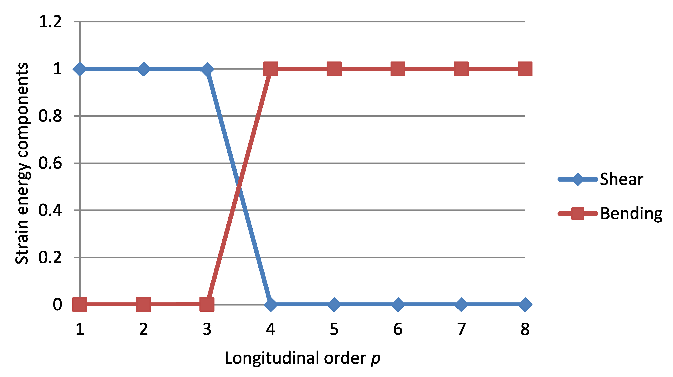
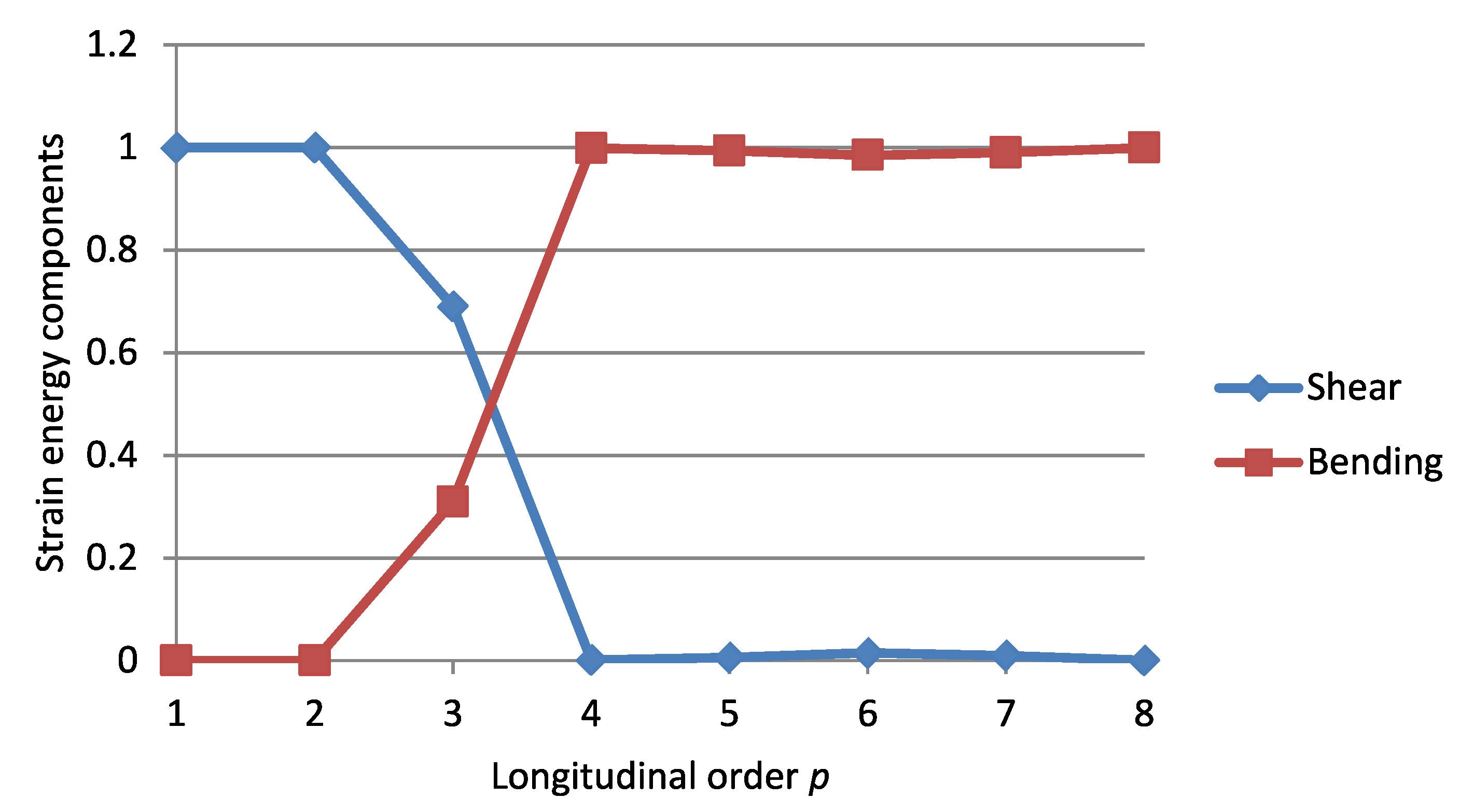
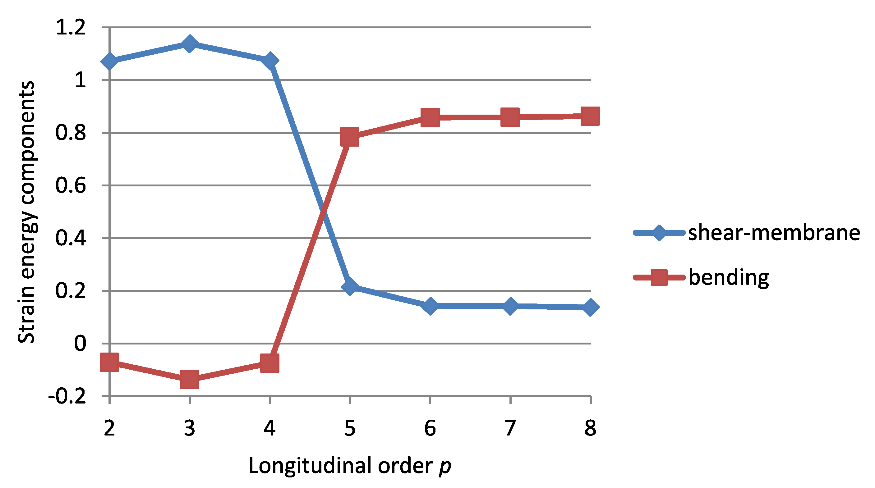
In our tests, we applied the results from the algorithms for the detection of the bending dominance. We calculated sums of elemental strain energy components present in the criterion (29). In the case of the plate problem, the shear and bending energy components were computed, while, in the shell examples, the sum of shear and membrane components and the bending component of the energy were determined. The assessed global plate problem was characterized with p = 1 , while in the shell examples the assessed global problems were characterized with p = 2 . Then, the energy components were calculated for the sequence of problems (30) characterized with P 1 = p , p + 1 , , 8 . The averaged values of the interelement stresses were used in the local problems definition. The transverse order of approximation corresponded to the second-order hierarchical shell model ( Q = q = 2 ) for all examples. The used mesh was characterized with H = h = l / 2 .
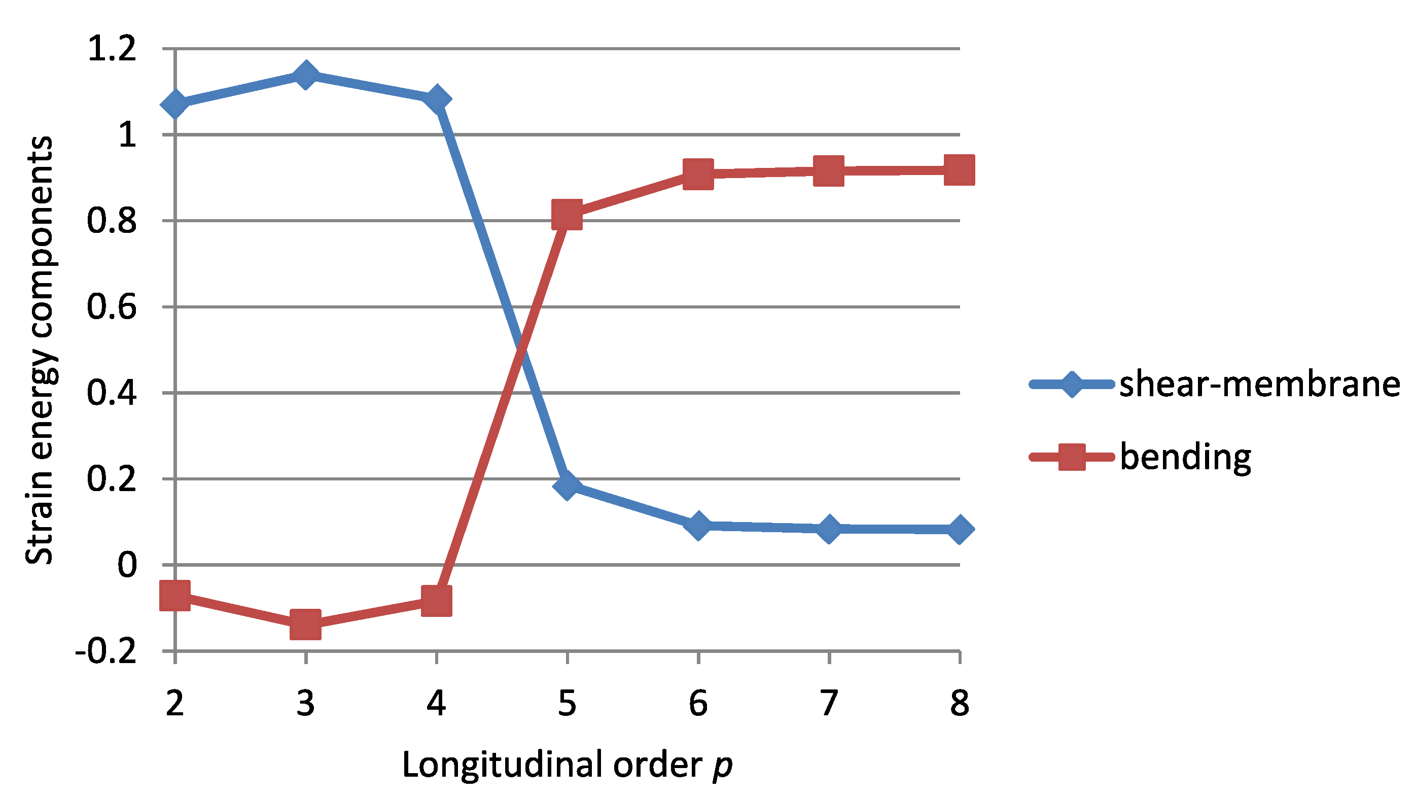
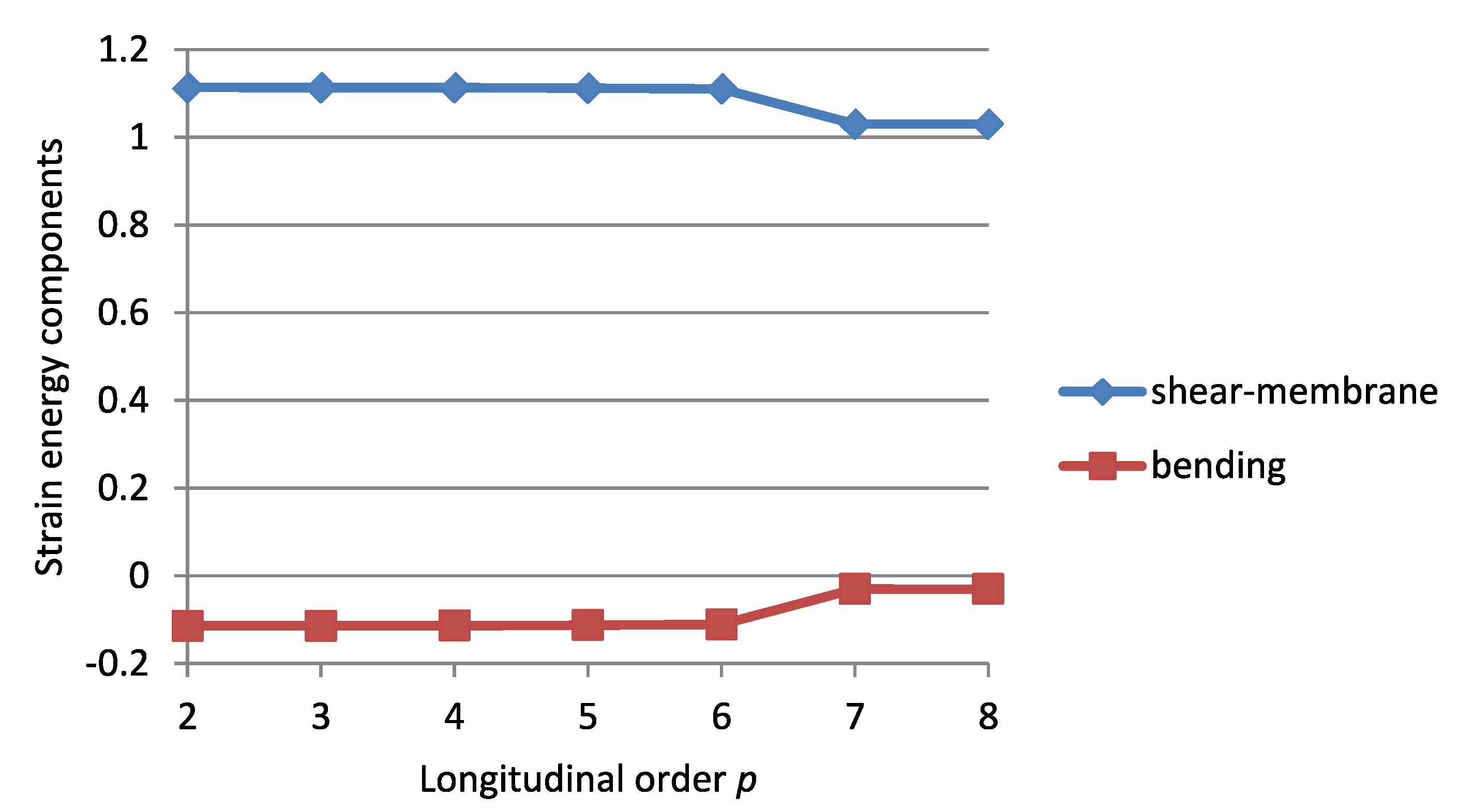
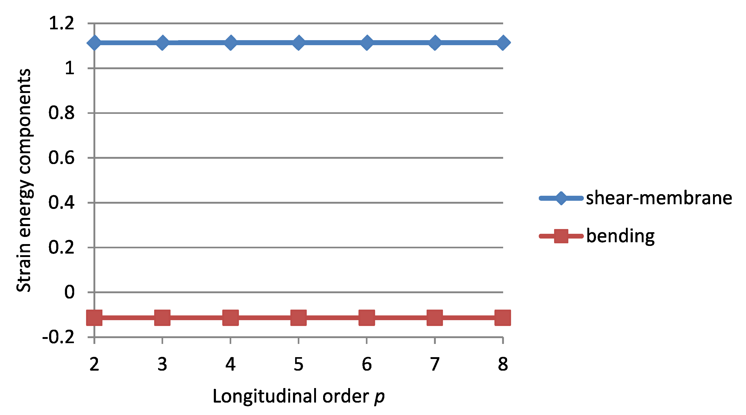
The above results from the sequence of the local problems were compared with the results from the global problems, where q = 2 and h = l / 2 . In the case of the plate, the following longitudinal orders of approximation were applied p = 1 , 2 , , 8 in the global problems, while in the case of two shell examples, the values of p = 2 , 3 , , 8 were taken into account. The results of the comparisons are presented in Figure 3, Figure 4, Figure 5, Figure 6, Figure 7 and Figure 8 for the plate and bending- and membrane-dominated shells, respectively. The figures present the ratios of the shear (the plate) or the sum of shear and membrane (the shells) energies to the entire strain energy and the ratios of the bending energy to the entire strain energy obtained from the local problems (top) and the global problems (bottom). Values of these ratios are presented versus the longitudinal order of approximation.
Comparison of the top and bottom figures for the model problems leads to the conclusion that the detection tools based on solution of the element local problems give practically the same results as the solutions to the global problems, both qualitatively and quantitatively. In both bending-dominated problems, the change of the membrane dominance resulting from the locking phenomena to bending dominance due to removal of the locking is perfectly indicated. In addition, the membrane-dominated problem has been perfectly identified, as shown by the third couple of figures—the membrane energy component dominates over the bending one for all values of the longitudinal order of approximation.

5. Effectivity of the Method in Model Problems

In this section, we present examples of application of the algorithms for detection and/or assessment of the locking phenomena, and the standard mesh modification algorithms as well, in the adaptive analysis of model problems. The adaptive procedure is derived from the three-step strategy [40] composed of the global solution and error estimation for the initial, intermediate (or h-) and final (or p-) steps. The global problems are based on 3D-based hierarchical modelling and approximations for complex structures [45]. Our models and approximations are related, based or derived from [30,31,41,42], respectively. The error estimation is performed using the equilibrated residual method [43,54], adjusted to the 3D-based formulation of the hierarchical models and approximations [46]. The three-step strategy is completed with the modification step performed after the initial one. The algorithms from the previous sections are used within this additional step. The averaged stresses are used instead of the equilibrated ones in the local problems.

5.1. Problems and Methodology

The three model problems in Section 4.1 are applied again. Two model bending-dominated plate examples are considered. In the first one, the data are exactly the same as in the mentioned section. In the second plate problem, we solve the plate of the same dimensions l / 2 and t as for a quarter of the plate from the first plate. In the second problem, all four lateral sides of the plate are clamped. In the first problem, two of them correspond to symmetry boundary conditions, and only two sides are clamped. In the second problem, one deals with the most coarse mesh possible and the lowest longitudinal order of approximation possible. As a result, the strongest possible locking appears for the assumed plate thickness. The third example is the bending-dominated shell from Section 4.1. The only difference is the shell thickness which is now equal to t = 0.003 × 10 2 m. The last example concerns the membrane-dominated shell. In this example, all data are exactly the same as in Section 4.1.

5.2. Numerical Examples

In the analysis of the locking phenomena, the following data were treated as independent: the problem type (the type of the strain dominance), and the structure length l and thickness t resulting in the thinness ratio l / t . In the numerical analysis, also the initial mesh data, the relative value of the target admissible error γ T , and the ratio γ I / γ T of the intermediate (after h-step) error to the target (after p-step) error were treated as independent quantities.
As results of the analysis, we present the meshes corresponding to three performed courses of adaptation: standard h p -adaptation and such adaptations preceded by the modification of the initial mesh with the increased longitudinal order of approximation p, equal either to the maximum or optimized value. The results are completed with the adaptive convergence curves corresponding to these three courses of adaptation. The convergence curves present the approximation error as a function of the number N of degrees of freedom (dofs). The absolute error is defined as a negative difference of the total strain energy U corresponding to the global solution under consideration and the reference energy U r replacing the unknown exact value. The energies are calculated in accordance with the strain energy definition from Section 2. Due to the exponential character of h p -convergence, the curves are plotted as log ( U r U ) versus log N . The reference energy U r is obtained numerically from calculations performed on over-killed meshes with the global discretization parameters equal to: p = 9 , q = 2 , m = 9 , where m = l / 2 h . Apart from the absolute error values, the relative error values ( U r U ) / U r are also presented and discussed.

5.2.1. A Quarter of a Bending Dominated Plate

Data

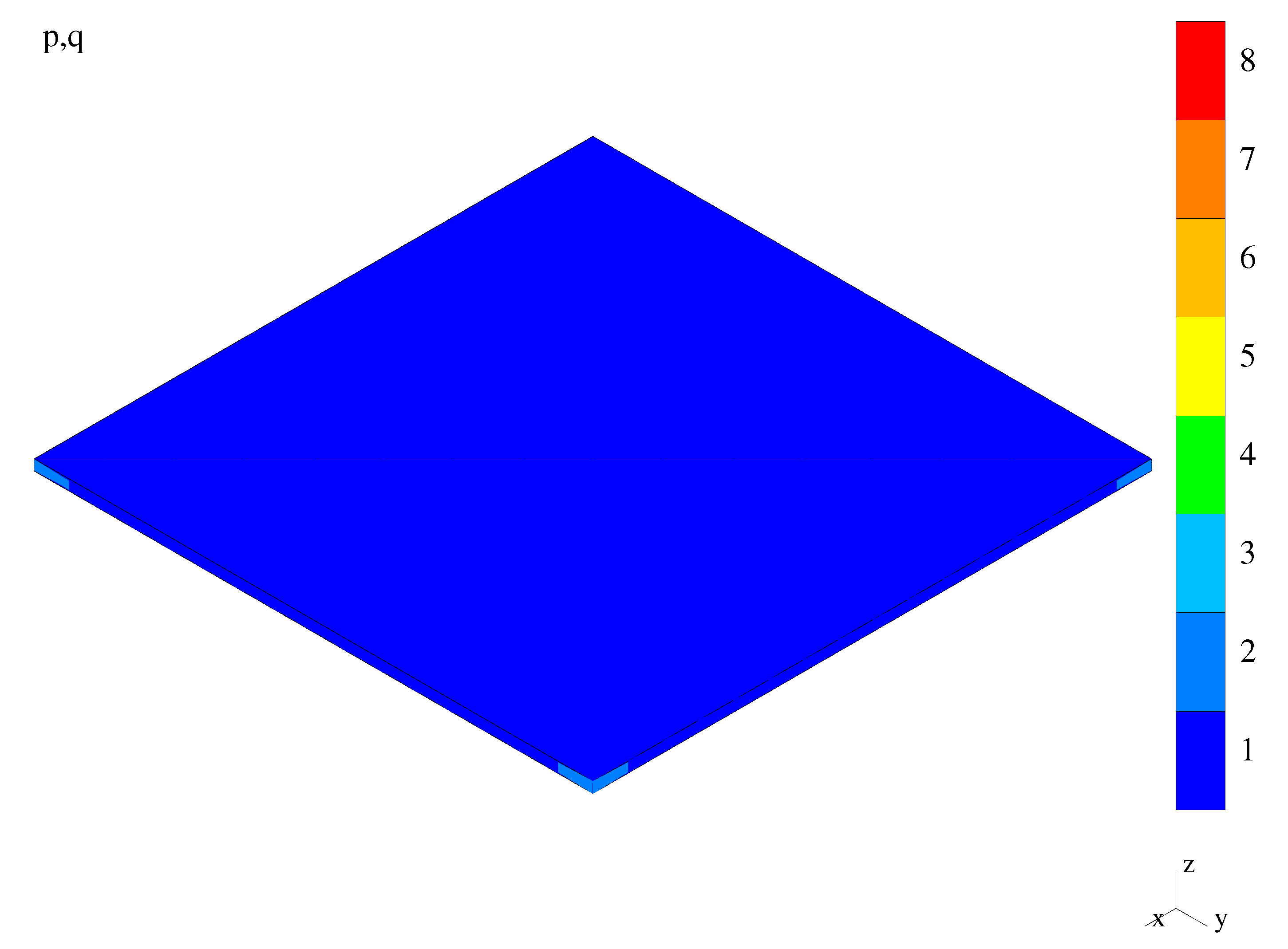
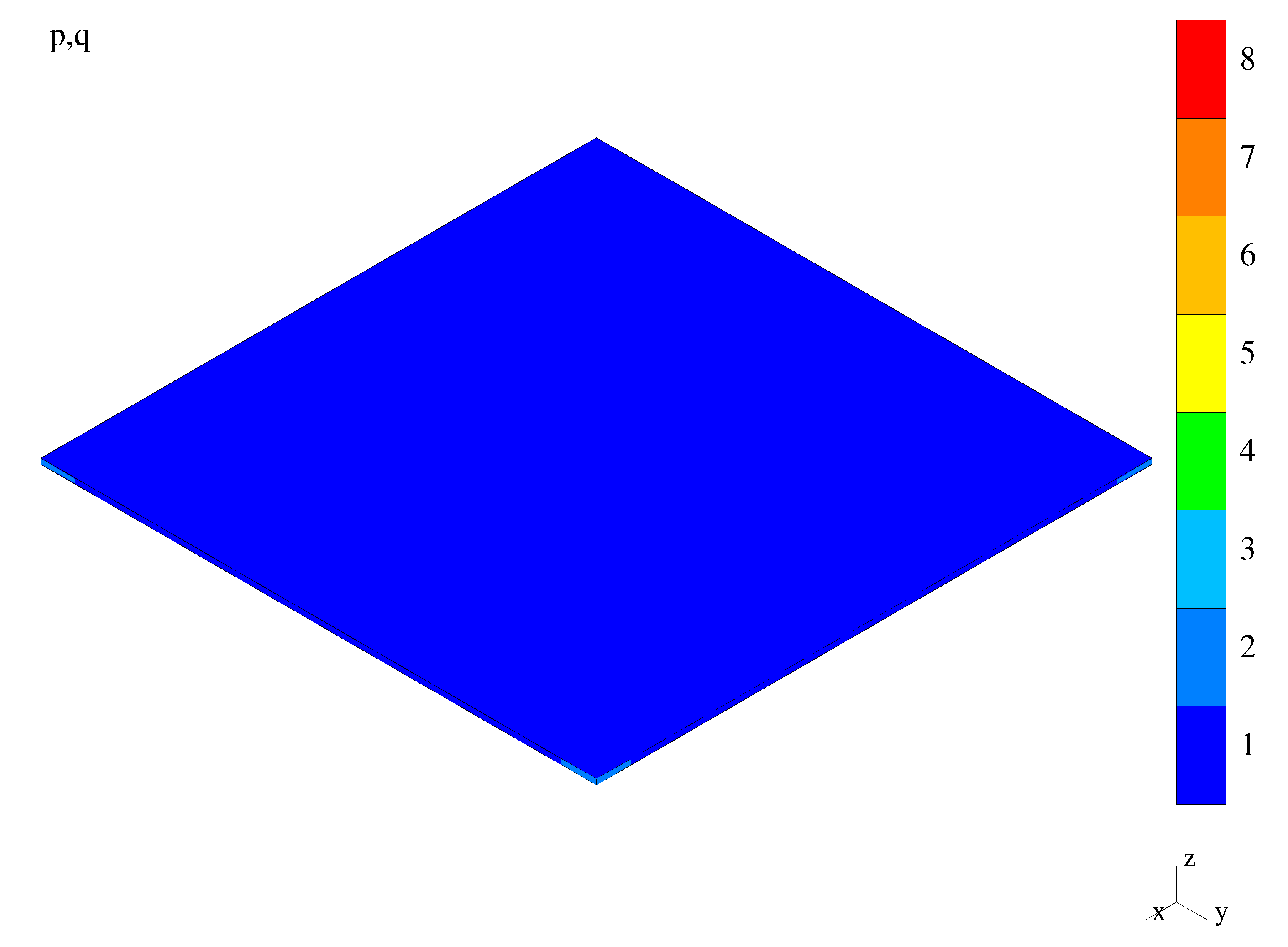
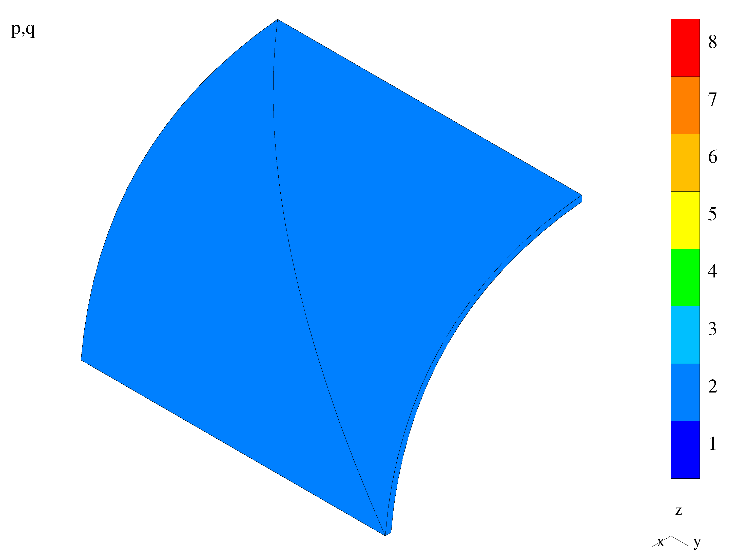
The dimensions of a quarter of the plate are such that the thinness ratio of the plate is l / t = 3.1415 × 10 2 / 0.03 × 10 2 . The initial mesh is coarse. Its data are as follows: the longitudinal approximation order p = 1 , the transverse approximation order q = 2 , and the element size h = l / 2 . This mesh is shown in Figure 9. In the error analysis, the target error γ T = 0.01 and the ratio γ I / γ T = 3 .

Results

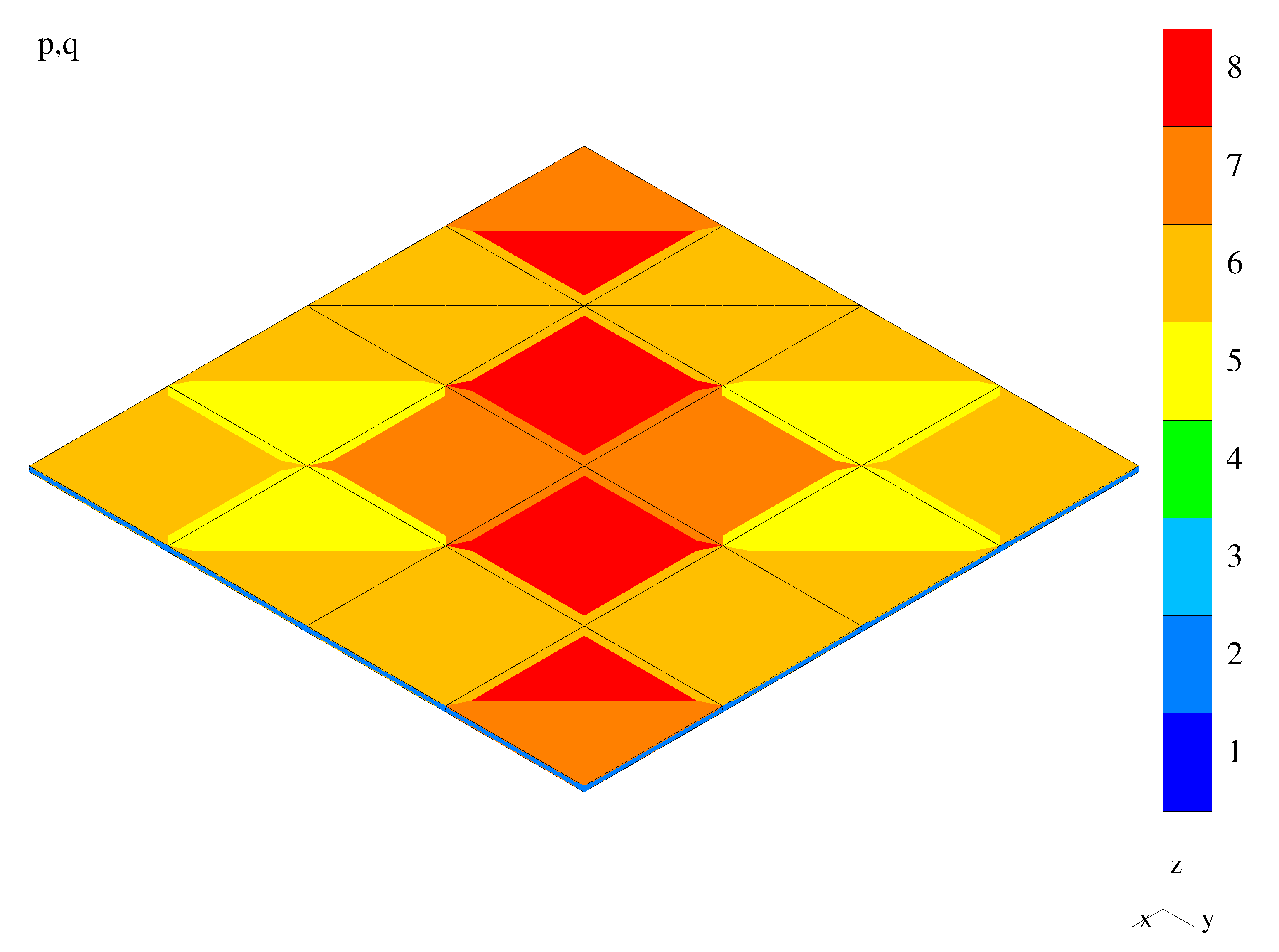
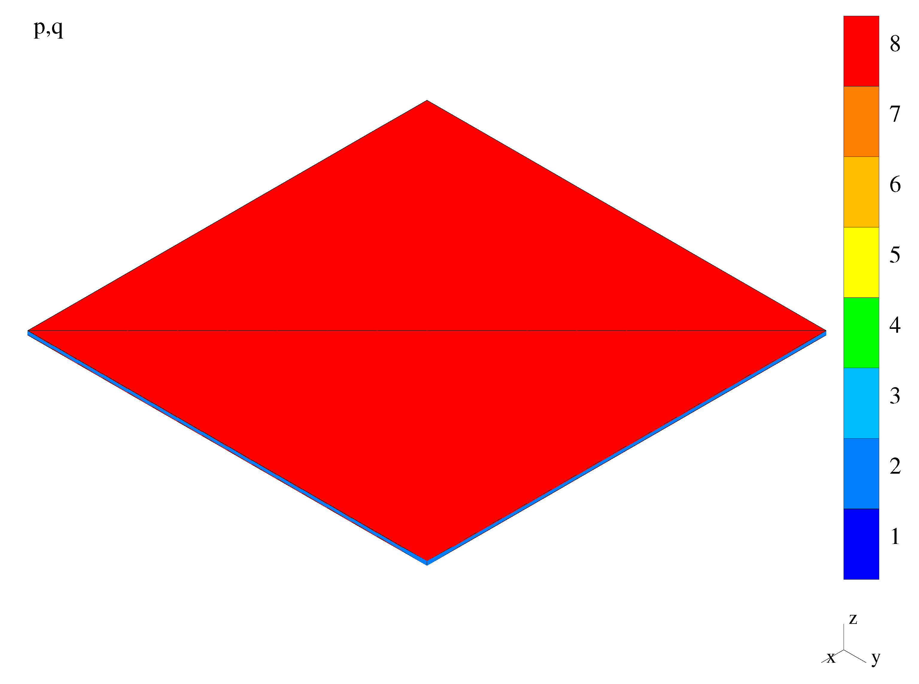
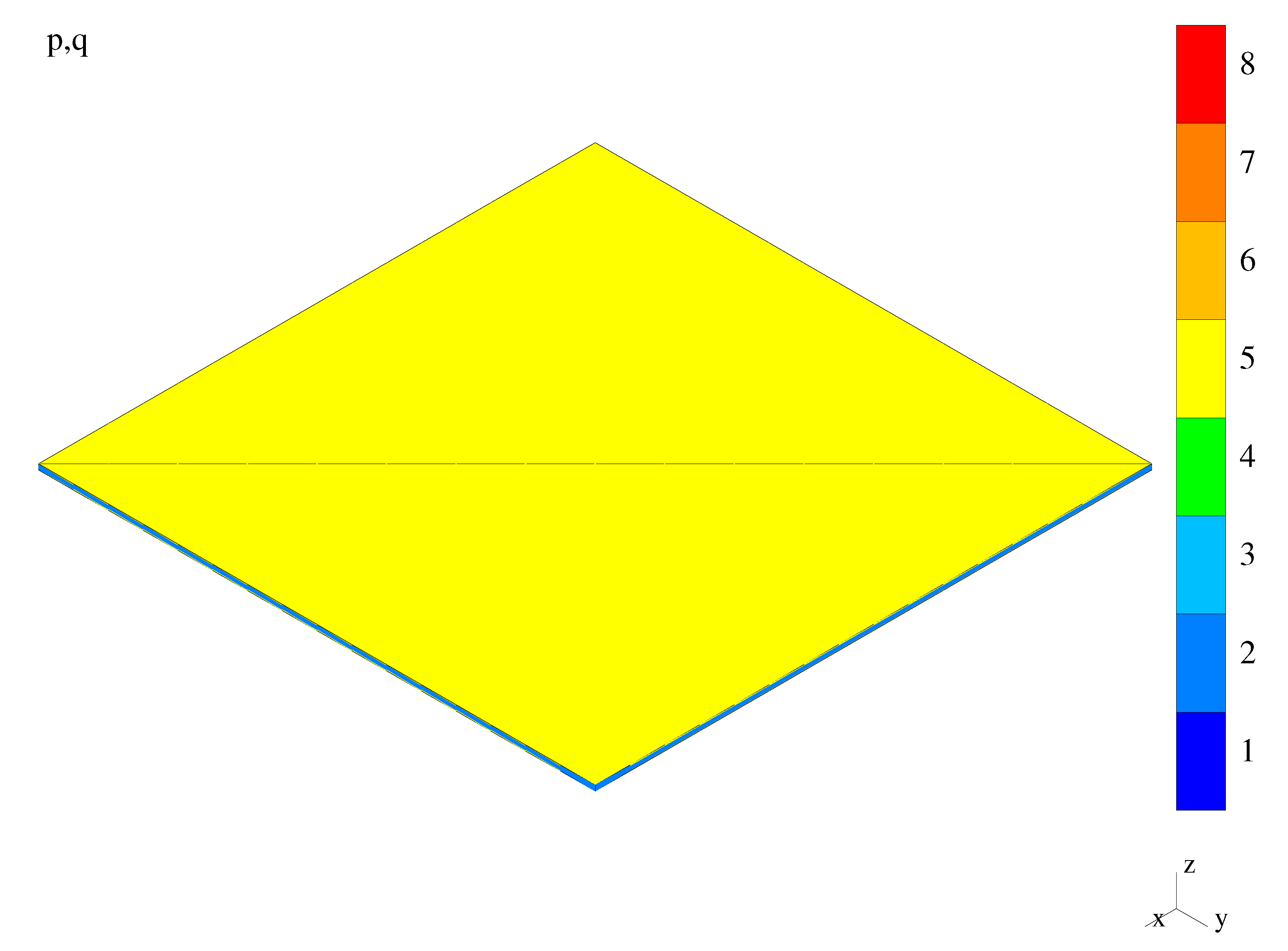
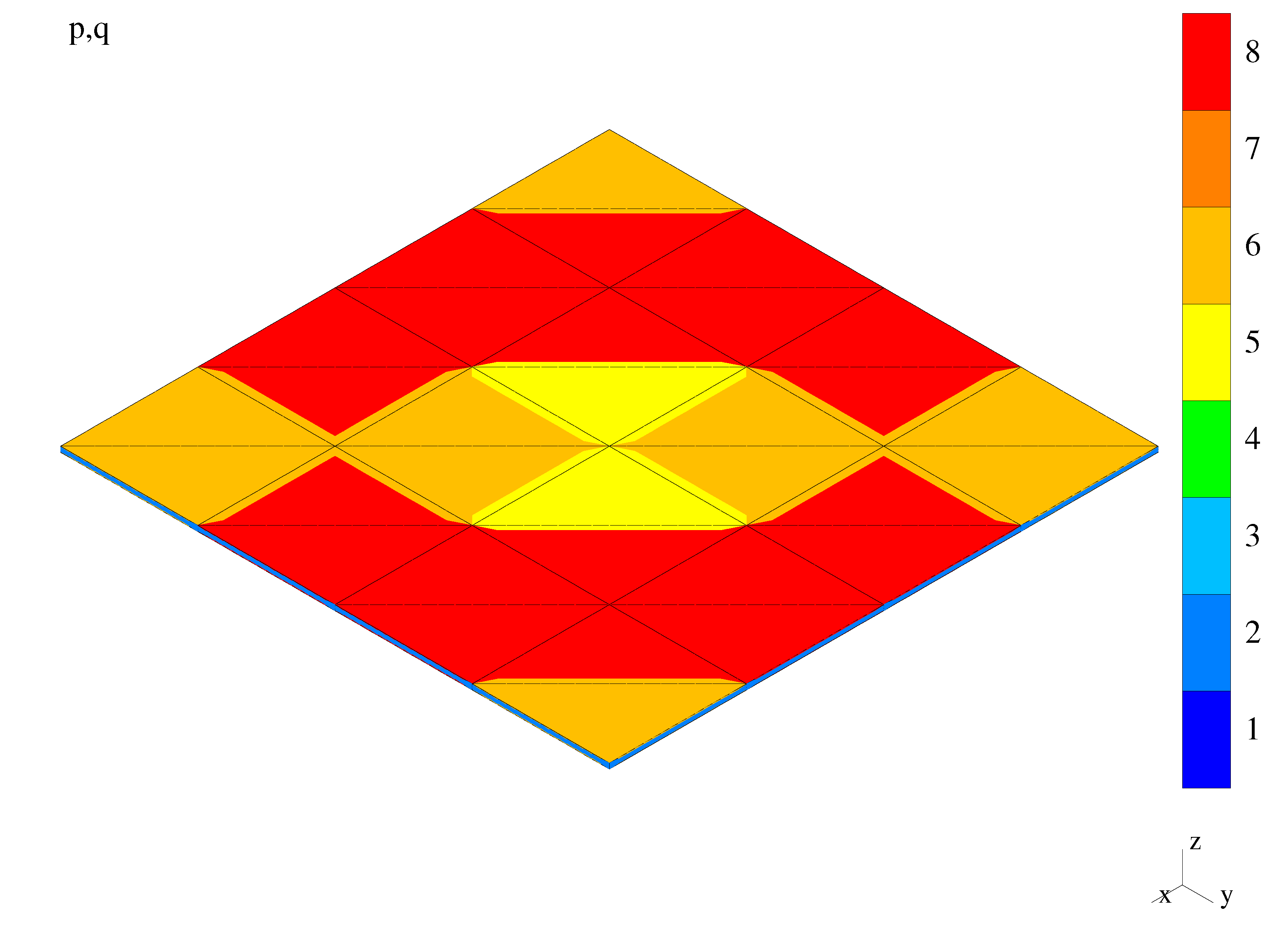
Three different courses of the adaptation are presented for this example. The first one corresponds to the standard h p -adaptivity composed of the h- and p-adaptation steps only. The final mesh for this first course is presented in Figure 10. The second course is the h p -adaptation preceded by the modification step based on the detection algorithm from Section 3.1.3, where, after the detection, the modification of the initial mesh is performed with the maximum setting p = 8 (Figure 11). No further automatic h-adaptation is performed by the adaptivity control algorithm. In addition, no further p-adaptation can be performed due to the maximum value of p applied in the modification step after the detection. The last course is the h p -adaptation performed after the initial mesh modification based on setting the longitudinal order of approximation to its optimized value p = 4 (Figure 12) obtained from the algorithm of Section 3.2.1. The final mesh completing this course of adaptation is presented in Figure 13. The not presented intermediate mesh possesses the same division pattern as the final mesh but the order of approximation is uniform and taken from the modified mesh ( p = 4 ).
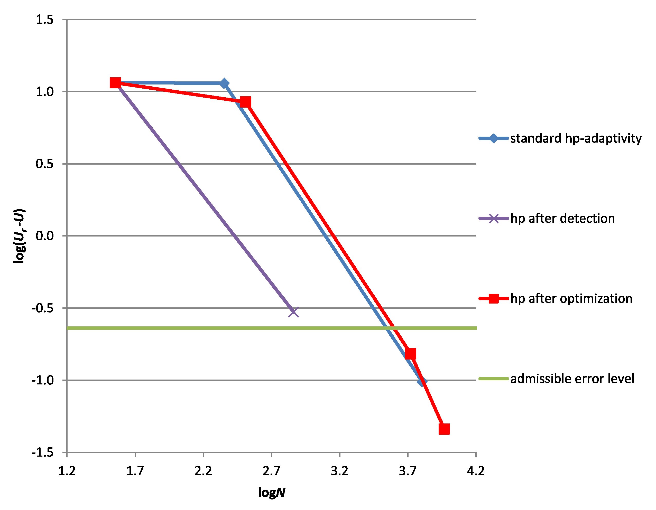
The adaptive convergence curves for three described cases are presented in Figure 14. In the case of the standard h p -adaptivity, the curve consists of two sections and three points corresponding to the initial, intermediate (h-adapted) and final ( h p -adapted) meshes. The influence of the shear locking is visible in the first section of the curve—this section is almost horizontal. In the case of the h p -adaptivity performed after detection of the locking and based on the modified value of p = 8 , two points of the convergence curve correspond to the initial and modified meshes. The locking has been removed—the only section of the curve is not horizontal. In the case of the h p -adaptation performed after the detection and optimization of the value of p, the convergence curve consists of four points (the initial, modified, intermediate, and final meshes) and three sections. The first not horizontal section of the curve reflects locking removal, while the next two sections correspond to h-refinement and p-enrichment.
Finally, it is worth mentioning that the automatic choice of the program may be the two courses with the initial mesh modification. These two automatic courses correspond to either the assumed maximum or determined optimized value of p applied in the modification step. The enforced course corresponds to the standard h p -adaptation.
The relations between the number N of degrees of freedom (dofs) and the absolute U r U and relative ( U r U ) / U r errors are summarized in Table 1 for the consecutive points of the three mentioned convergence curves. The mesh figure numbers corresponding to these points are also indicated.

Discussion

The shear locking has been detected in both cases which include modification of the initial mesh based on the maximum and optimized values of the longitudinal order p. One can see that the standard h p -adaptation leads to the final error value below the desired admissible value of γ T . The same refers to the h p -adaptation preceded by the modification based on the optimized value of the longitudinal order of approximation p = 4 . In the case of the h p -adaptation performed after the modification of the mesh based on the fixed maximum value of p = 8 , the admissible error value has not been reached, even though the error has been diminished. The reason is the discrete character of the possible h-adaptation. For the estimated error level, this adaption has not been performed.

5.2.2. A Bending-Dominated Plate

Data

In this example, the entire plate is considered. Thus, the thinness ratio is equal to l / 2 t = 1.57075 × 10 2 / 0.03 × 10 2 . The discretization parameters of the coarse initial mesh, i.e., the element longitudinal and transverse approximation orders and the element size, are p = 1 , q = 2 , and h = l / 2 , respectively. These parameters can be seen in Figure 15. The data for the error analysis are assumed as: the admissible target error γ T = 0.02 and the ratio of the admissible intermediate to admissible target errors γ I / γ T = 3 .

Results

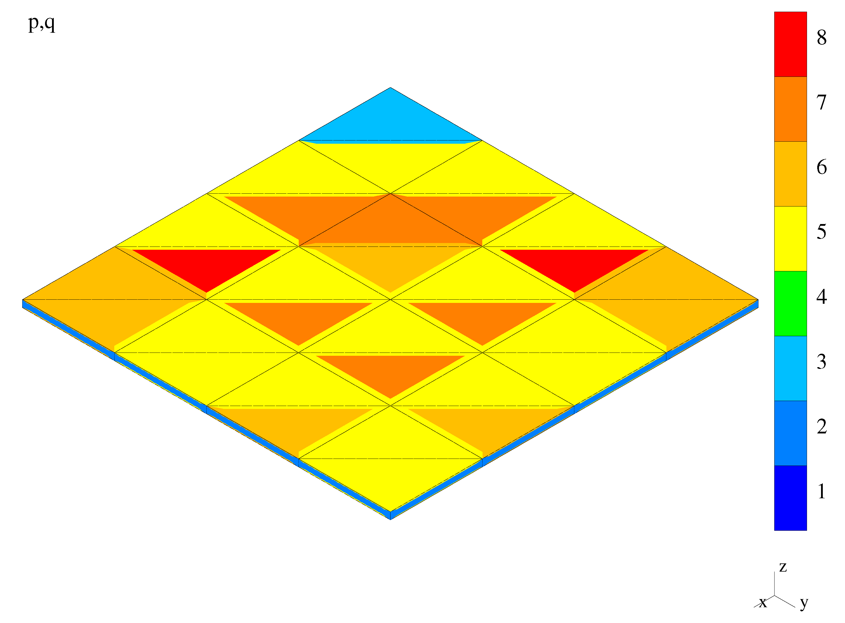
As in the previous test, three courses of adaptation are of our interest. The first course corresponds to the standard h p -adaptivity where the initial mesh is h- and then p-adapted. The h p -adapted final mesh is shown in Figure 16. The next course of the adaptation is based on the h p -adaptation which is preceded by the modification of the initial mesh. This modification (Figure 17) lies in setting the longitudinal order of approximation as equal to the maximum possible value removing the locking, i.e., p = 8 , after the phenomenon has been detected by means of the algorithm of Section 3.1.3. As in the previous example, no further adaptive actions have been performed. The h-division has not been made due to the estimated approximation error level and discretized character of performance of the adaptivity control algorithm. The p-enrichment has not been possible as the maximum value of p = 8 has already been applied in the modified mesh. The third course of adaptation consists of the h p -adaptation following the modification of the initial mesh by adopting the optimized value ( p = 5 ) of the longitudinal order of approximation (Figure 18). This value was established by the algorithm from Section 3.2.1. The final mesh for this adaptation is presented in Figure 19. The not displayed intermediate mesh has the same division pattern as the final mesh and the longitudinal approximation order as in the modified mesh, i.e., p = 5 .
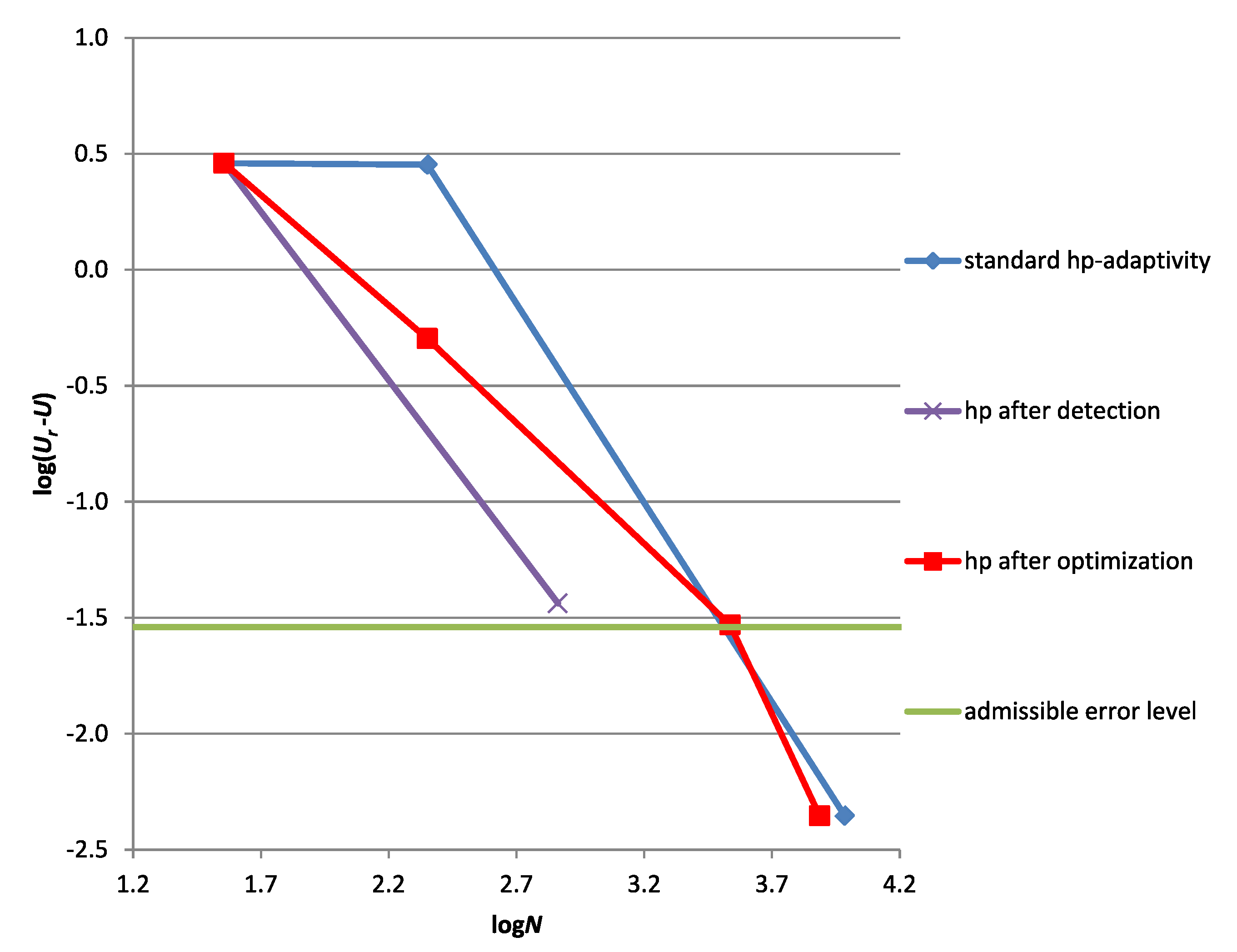
The convergence curves corresponding to the performed adaptations are displayed in Figure 20. In the case of the standard h p -adaptivity, the curve consists of three points and two section. These three points correspond to three meshes generated within this course: the initial, intermediate (or h-adapted), and final (or h p -adapted) ones. The presence of the shear locking is reflected by the first horizontal section of the curve. In the case of the h p -adaptivity performed after detection of the locking and applying the modified maximum value of the longitudinal order of approximation, i.e., p = 8 , the convergence curve consists of two points and one section. These two points correspond to the initial and modified meshes. In the only section of the curve that is not horizontal, he locking has been removed. In the third course of adaptation, based on the modification of the initial mesh by the optimized value of the approximation order p = 5 , the convergence curve consists of three sections and four points—the initial, modified, intermediate, and final meshes have been generated. It can be seen that the locking has been removed as the first section is not horizontal.
It should be stressed that the modes including modification step are the automatic choice of the adaptive algorithm, while the standard h p -adaptivity is the enforced mode.
In Table 2, the relations between the number N of degrees of freedom and the absolute and relative errors, respectively, U r U and ( U r U ) / U r , are presented for the consecutive points of the convergence curves of three adaptation modes. The mesh figure numbers corresponding to these points are also indicated in the table.

Discussion

Firstly, as expected, the shear locking has been detected. Secondly, the adaptation based on modification of the initial mesh by the optimized value of the longitudinal order of approximation leads to final error value below the admissible error value, in contrast to the modification based on the maximum value of the longitudinal order of approximation p = 8 . Again, the discrete values of parameters controlling the adaptation process have resulted in no further adaptation after the initial mesh modification. One can see, however, that the standard h p -adaptation leads to the final error level below the admissible value again. We show in the next example that this is not the rule.

5.2.3. A Quarter of a Bending-Dominated Shell

Data

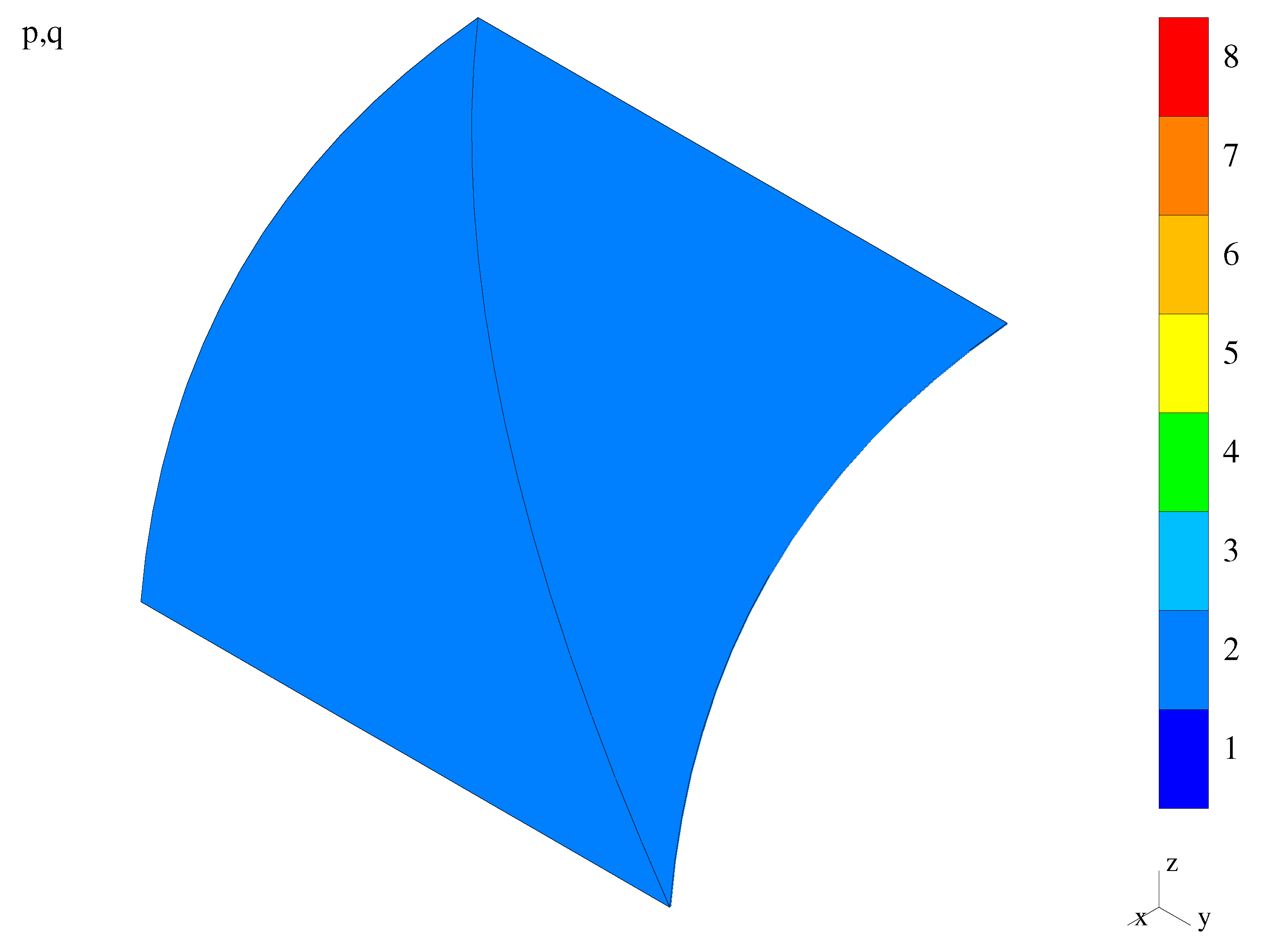
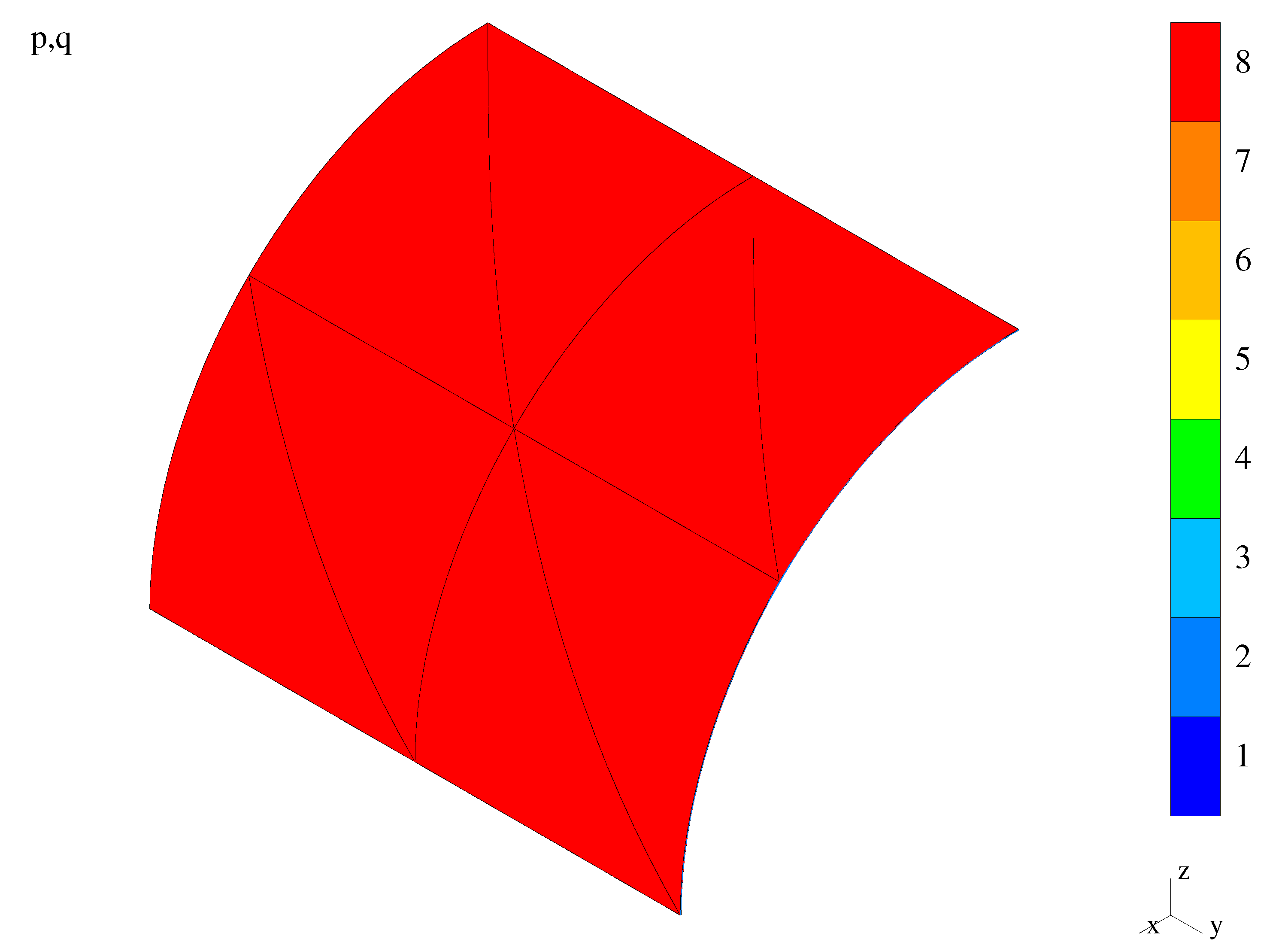
This example concerns a symmetric quarter of the half-cylindrical shell. The thinness ratio for this structure is equal to l / t = 3.1415 × 10 2 / 0.003 × 10 2 . We assume the following discretization parameters: the longitudinal order of approximation p = 2 , the transverse one q = 2 , and the element size h = l / 2 . The shell quarter and its initial discretization is illustrated in Figure 21. The error analysis is based on the following assumptions: γ T = 0.007 and γ I / γ T = 3 .

Results

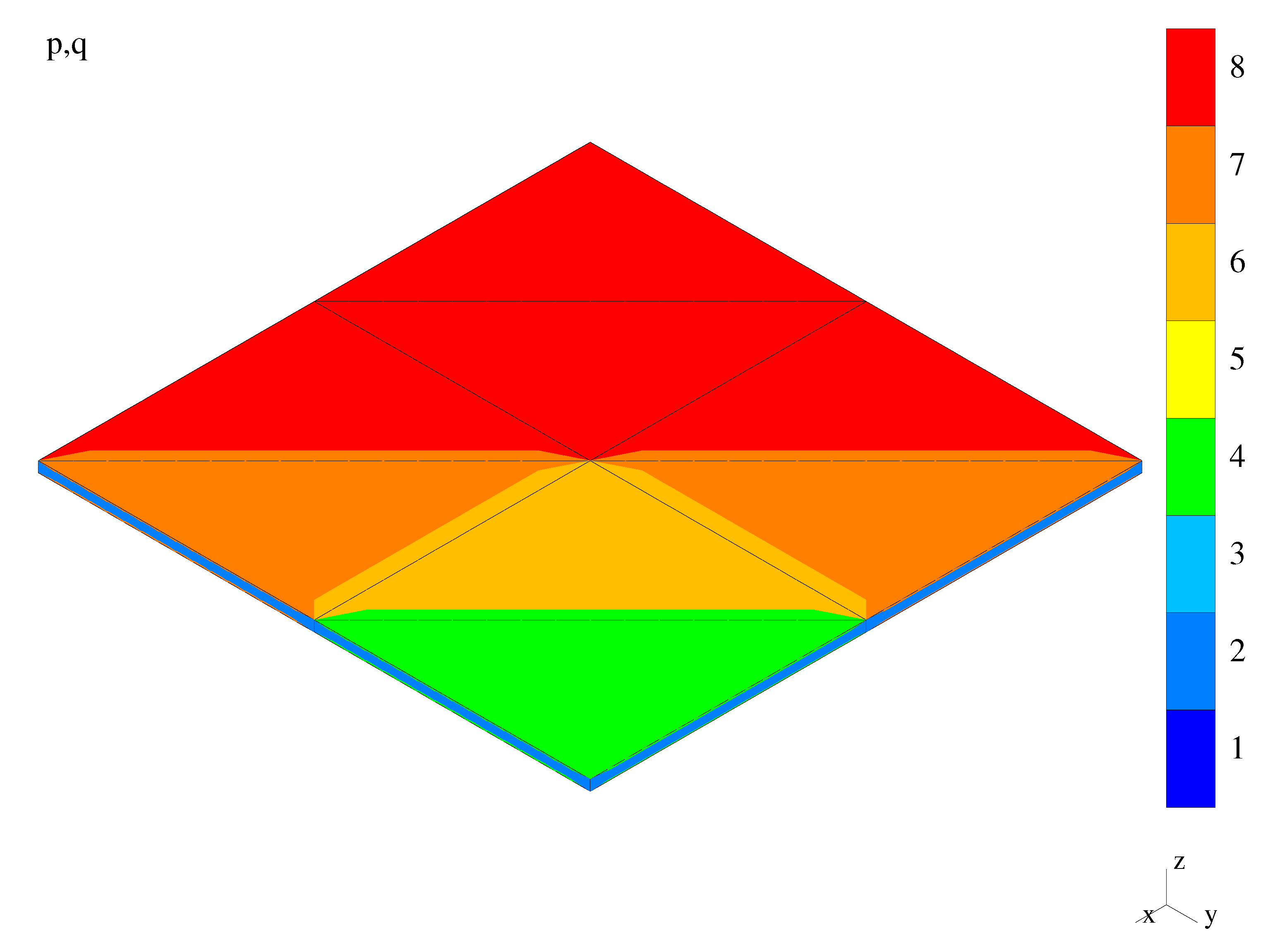
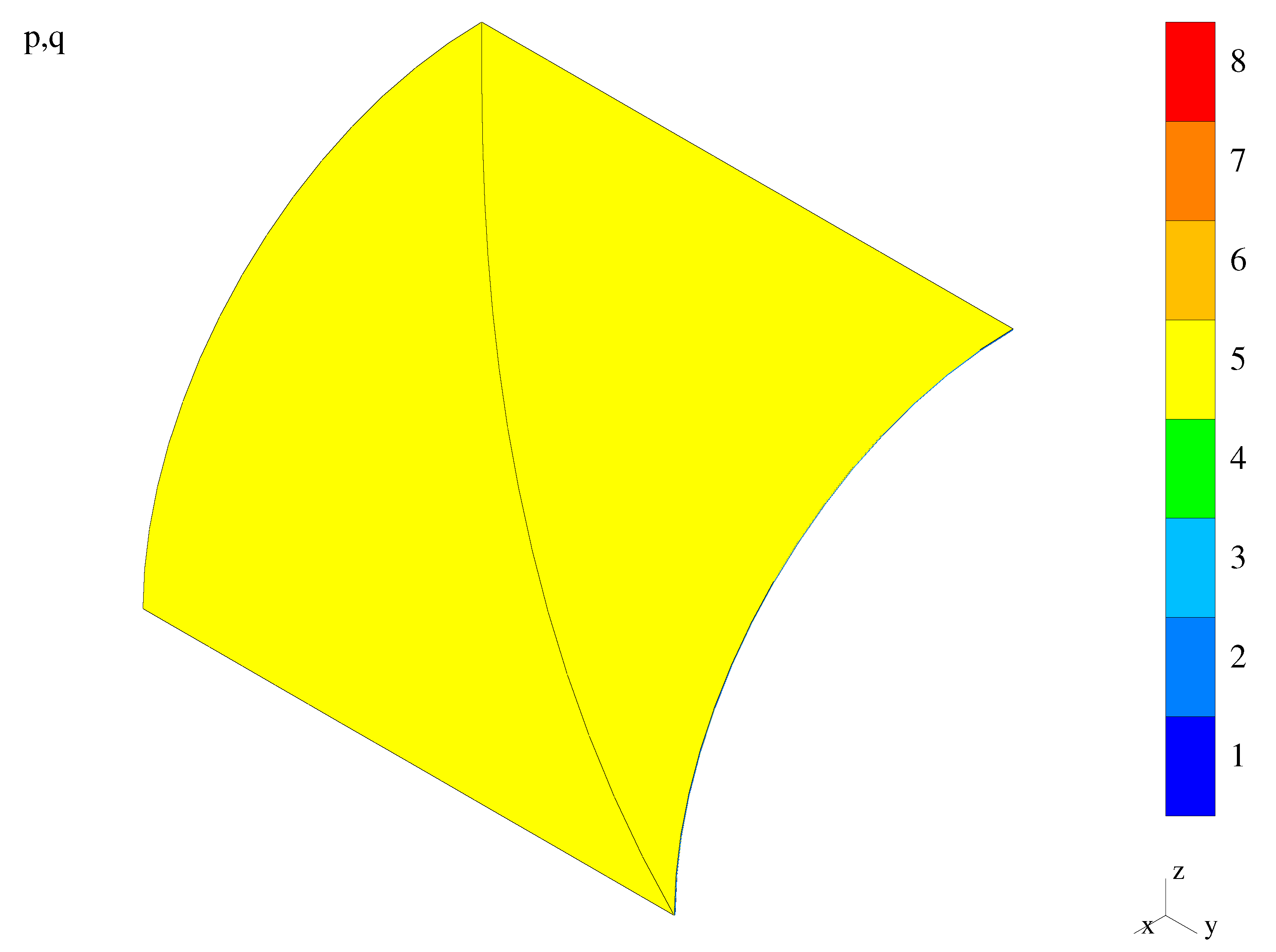
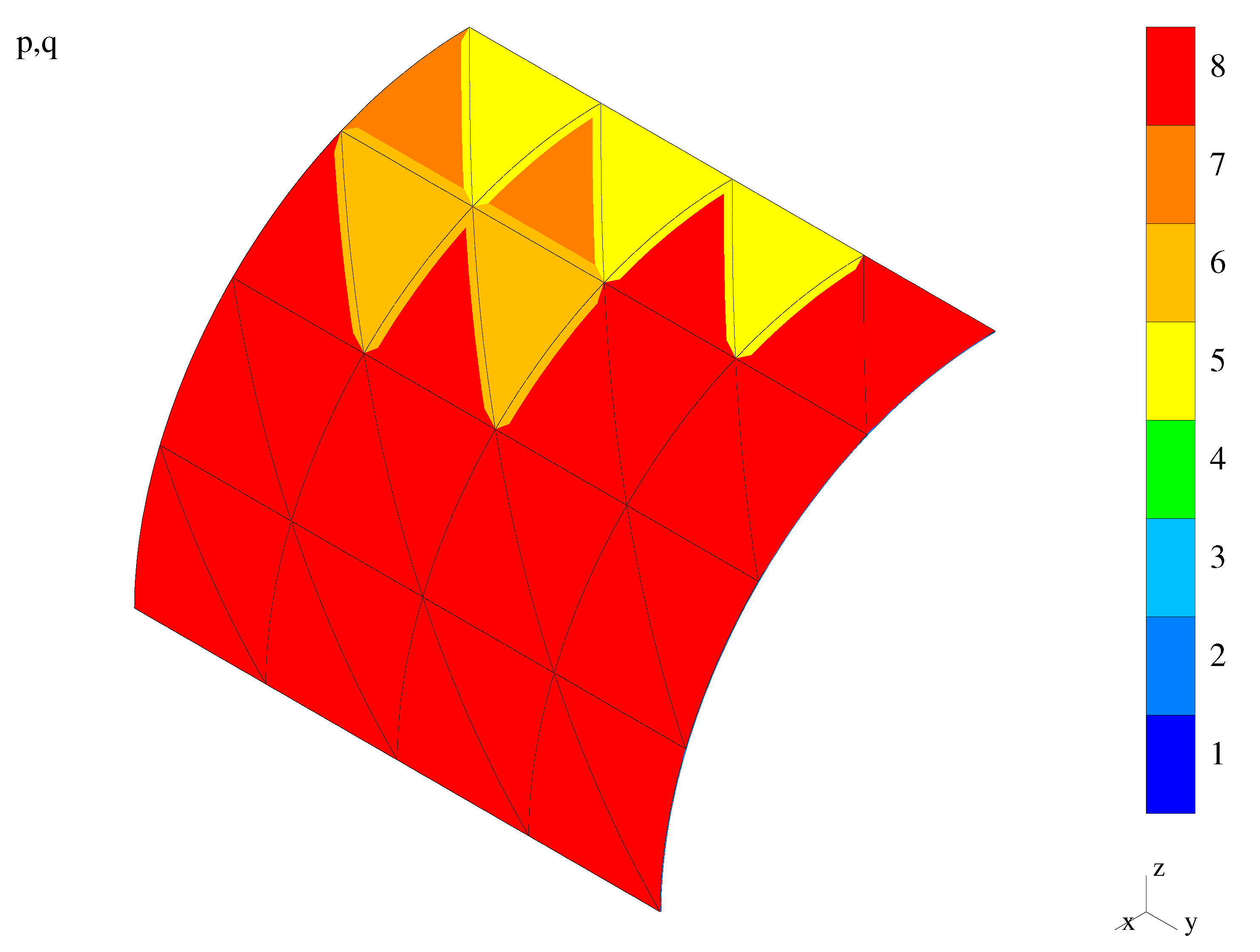
As in the previous two bending-dominated examples, also here three courses of the adaptation are performed. The first adaptation is the standard procedure composed of h- and p-steps. The mesh after h p -adaptation can be seen in Figure 22. The second and third types of the adaptation are composed of the h p -adaptation which follows the modification of the initial mesh. In the second type, the modification is based on the maximum possible value of the longitudinal order of approximation p = 8 (the corresponding figure is not displayed). In the case of the second type of adaptation, the modified mesh has been h-adapted further (see Figure 23). In the third type, the modification takes advantage of the optimized value of p = 5 (Figure 24). In the second type, the p-adaptation has not been possible as the maximum value of p = 8 has already been applied. In the third type of adaptation, the modified mesh has been h p -adapted. The final mesh is presented in Figure 25. The not revealed intermediate mesh possesses the same division pattern as the final mesh and the uniform order of approximation as in the modified mesh, namely p = 5 .
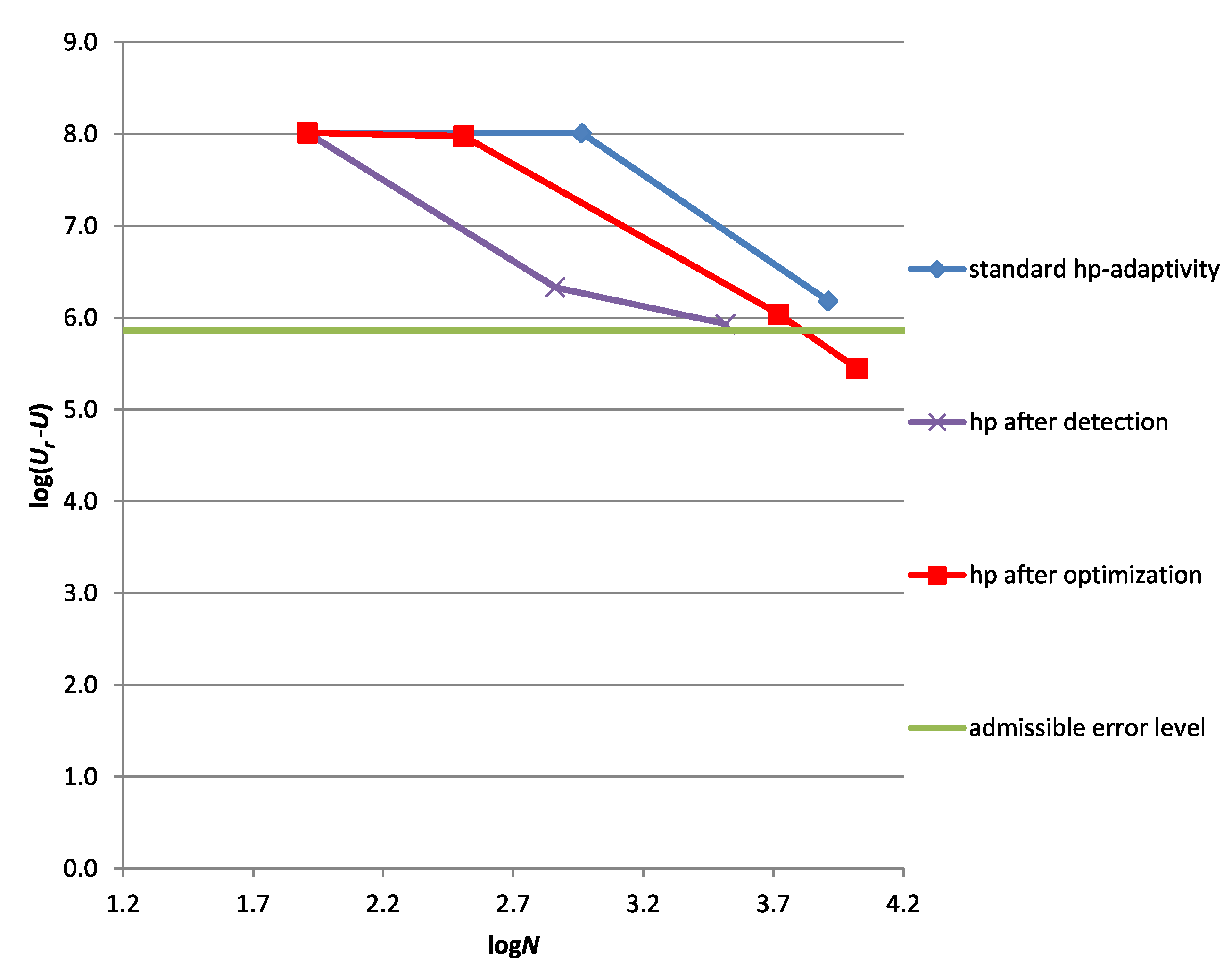
Three convergence curves resulting from the described adaptations are presented in Figure 26. The standard h p -adaptivity convergence curve consists of two sections and three points indicating the estimated error level for the initial, intermediate, and final meshes. In the case of the h p -adaptation following the modification based on the maximum value of p = 8 , the curve consists of two sections and three points corresponding to the initial, modified, and h-adapted (intermediate) meshes. The shear–membrane locking has been removed—the first section of the curve is not horizontal. In the last case of the h p -adaptivity following the modification based on the optimized value of p = 5 , the curve is composed of three sections and four points—the initial, modified, intermediate, and final meshes have been generated. The locking has not been removed from the modified mesh, however the value of p = 5 has appeared sufficient for removal of the locking from the h-adapted (intermediate) mesh—the second section of the convergence curve is not horizontal.
Note that the adaptations including the described mesh modifications, based on either the maximum ( p = 8 ) or optimized ( p = 5 ) values of the longitudinal order of approximation, may be performed automatically by the program, while the standard h p course has to be enforced by a user.
As in the previous numerical examples, the absolute and relative error values, respectively, log ( U r U ) and ( U r U ) / U r , are presented in Table 3 versus the number N of degrees of freedom (dofs). For the points of three adaptive convergence curves, the corresponding mesh figure numbers are included in the table.

Discussion

The anticipated shear–membrane locking has been detected in two adaptation modes including modification of the initial mesh. In the case of the standard h p -adaptation, the admissible error value has not been achieved. This is because the estimated error level and the discretization parameters in the adapted meshes have not been determined accurately due to the locking. In the adaptation with modification based on the maximum p possible, the admissible error value has not been achieved. This is because only further h-adaptation has been performed and further p-adaptation has not been possible as the maximum value of p = 8 has already been adopted. However, the admissible error value has been confidently achieved in the adaptation with the modification of the initial mesh based on the optimized value of p.

5.2.4. An Octant of a Membrane-Dominated Shell

Data

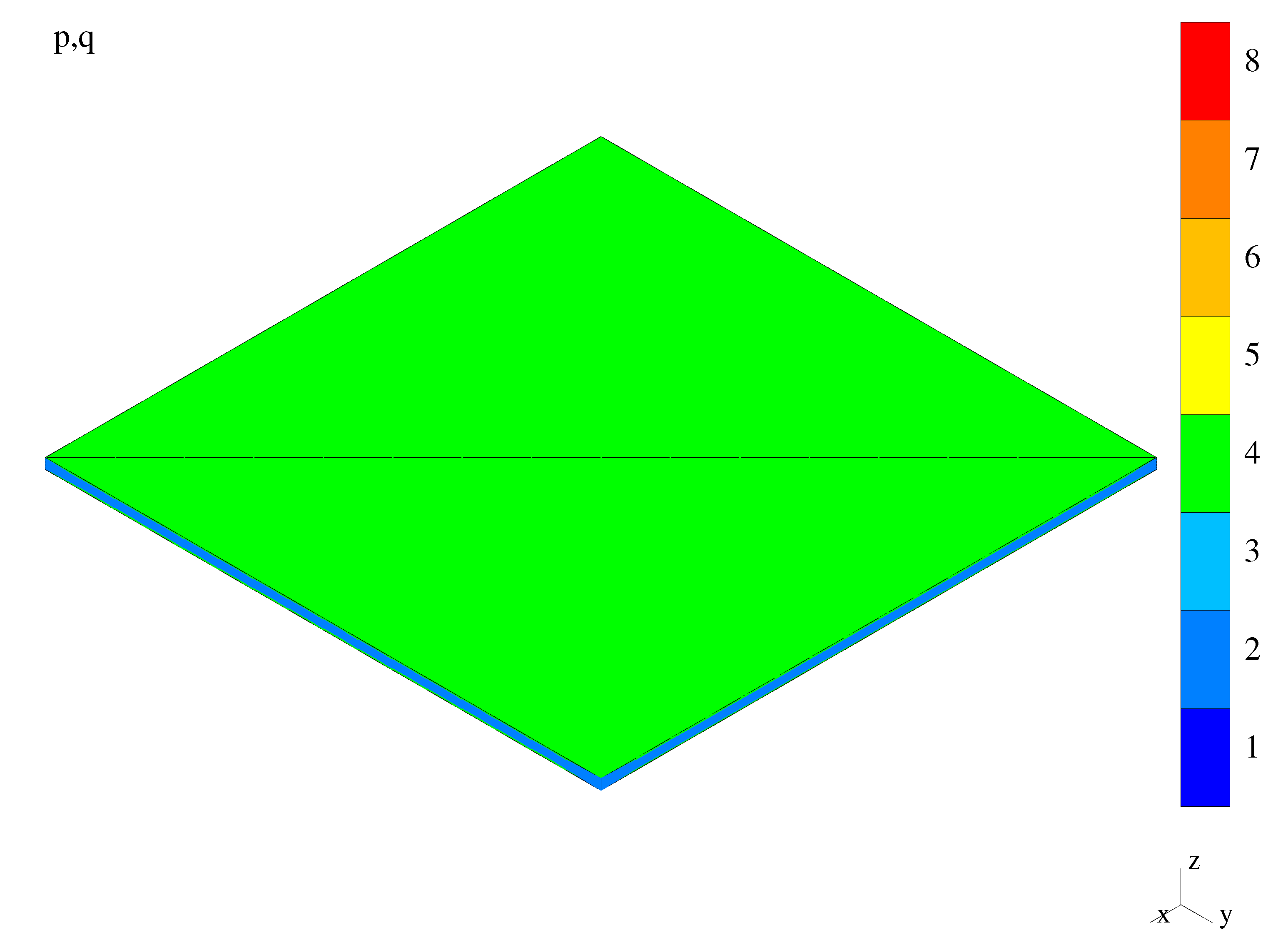
A symmetric octant of the cylindrical shell and its initial discretization, based on p = 2 , q = 2 , and h = l / 2 , are presented in Figure 27. A very coarse initial mesh can be seen in this figure. The thinness ratio equals l / t = 3.1415 × 10 2 / 0.03 × 10 2 . The error data controlling the h p -adaptation are the admissible relative error value on the final mesh γ T = 0.01 and the ratio of the admissible error values on the intermediate and final meshes γ I / γ T = 2 .

Results

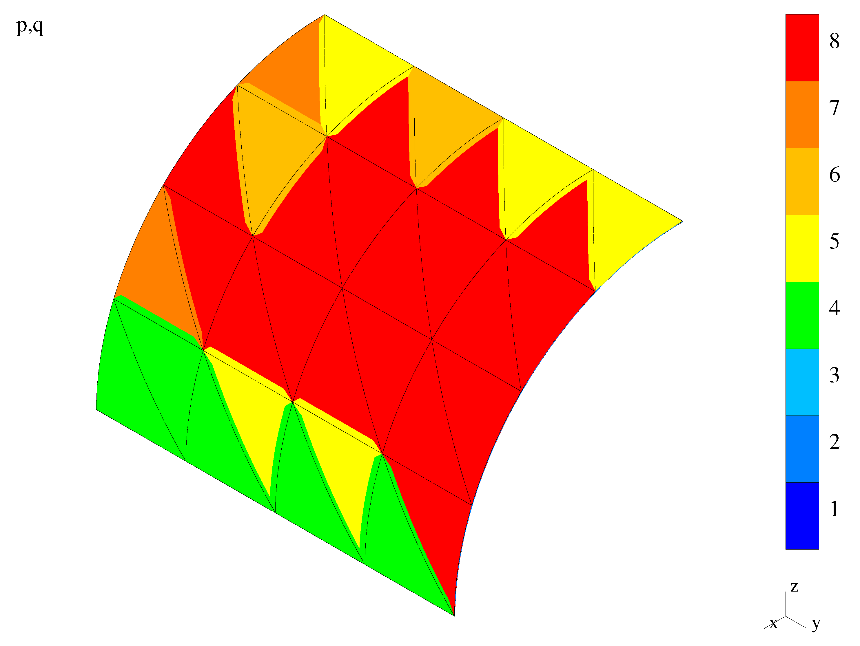
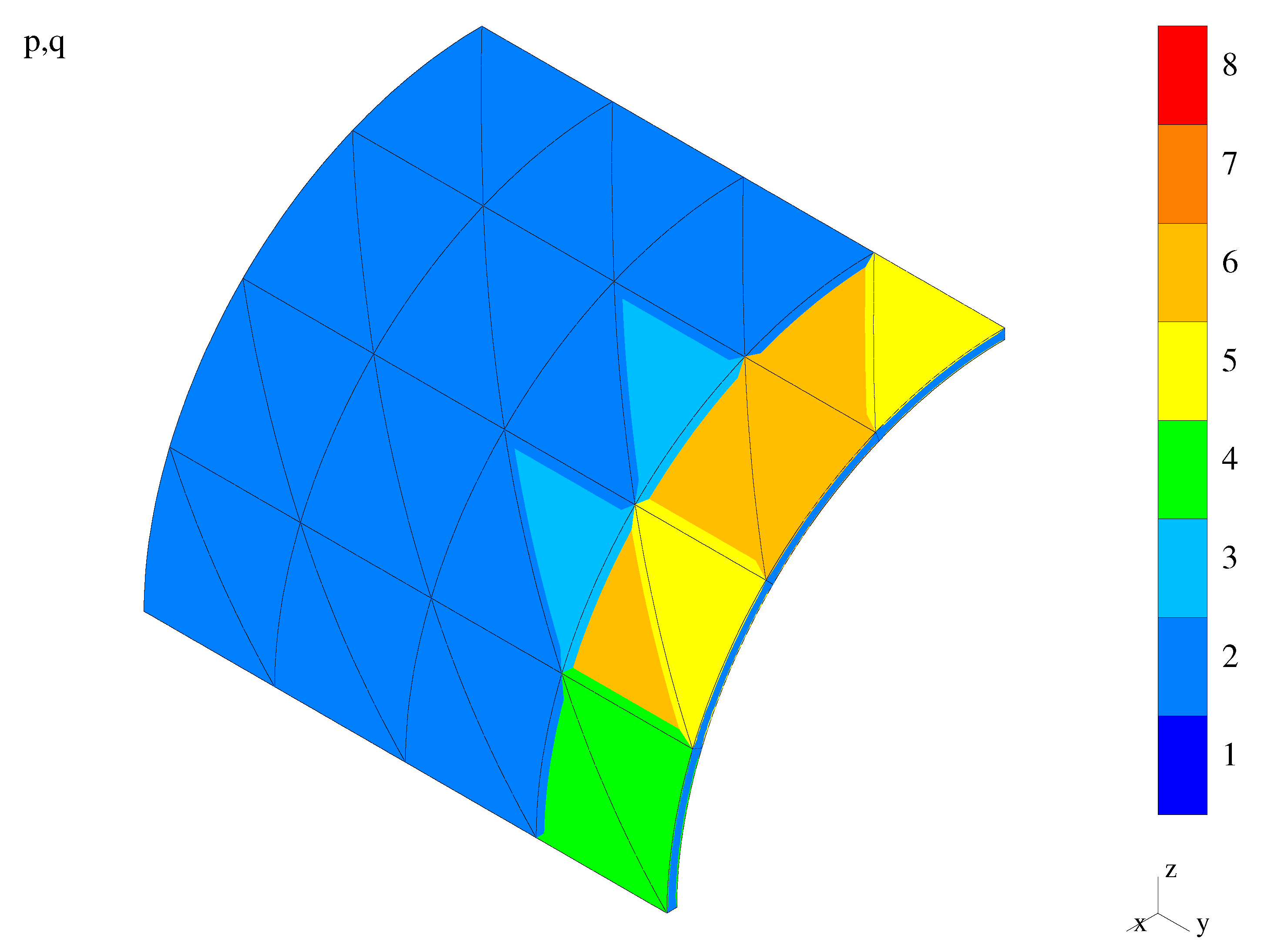
As expected, the automatic tools for detection and/or assessment of the locking have not indicated the appearance of the phenomenon. Because of this, the automatic mode of adaptation corresponds to standard h p -approach. The final, h p -adapted mesh is presented in Figure 28. Note that the intermediate (h-adapted) mesh is not presented but it can easily be obtained from the results in Figure 27 and Figure 28 by taking approximation orders p and h-division pattern from these two figures, respectively. It can be seen in the presented figure that, in the vicinity of the curved edge with the rotations constrained, the higher error level and the resultant higher approximation orders are present due to the local bending along the constrained boundary. The membrane and bending strain energies are of the same order along this boundary. In the rest of the shell octant, the membrane strains dominate over bending ones and the error level is lower and evenly distributed. Because of this, the resultant approximation orders are also lower and evenly distributed.
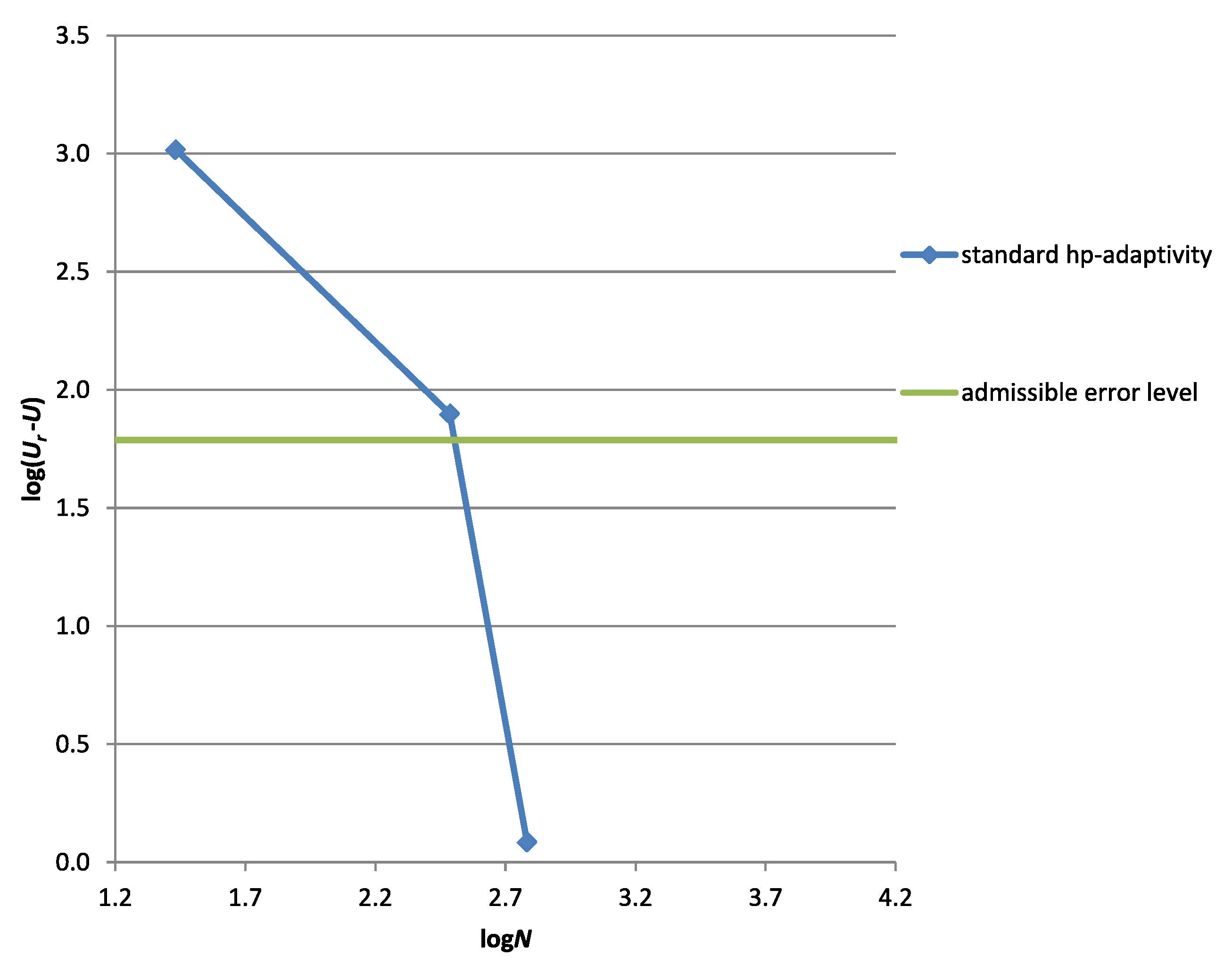
The convergence curve corresponding to the standard three-step h p -adaptivity is shown in Figure 29. The first point on the curve corresponds to the initial mesh. The second point of the curve is for the intermediate mesh, while the third point for the final mesh. The admissible error value was confidently achieved in the corresponding three steps.
Finally, in Table 4, the summarizing results of the absolute error U r U and the relative error ( U r U ) / U r are presented versus the number N of degrees of freedom (dofs) for three points of the convergence curve. The mesh figure numbers corresponding to these points are also included in the presented table.

Discussion

It can seen that the locking detection and/or assessment tools are capable of not only detecting the phenomena but also recognizing the problems where the phenomenon is not present. Such a result of the detection is consistent with theory presented in the literature (compare [32]). In situations such as this, performance of the standard h p -approach is enough to achieve the admissible error value as shown in this example.

5.2.5. Generalizations

Based on the above representative examples, and other analogous examples performed by the authors and not presented here due to their qualitative and quantitative similarity, one can state that:
  • The adaptation mode based on standard h p -adaptivity may fail when applied to the problems where the locking phenomena are present.
  • The adaptation mode which allows modification of the initial mesh with the maximum possible longitudinal order of approximation may lead to underestimation of the final error value.
  • The course of adaptation with the modification of the initial mesh by means of the optimized value of the longitudinal order of approximation is more effective in achieving the admissible error value than the previous two courses of adaptation.

6. Conclusions

The proposed tools for detection and/or assessment of the locking phenomena are capable of the detection of the shear locking and shear–membrane locking as well. These tools are also capable of recognizing the problems without locking phenomena present.
The removal of the locking phenomena by modification of the initial mesh, based on the optimized value of the longitudinal order of approximation p, can effectively lead to the admissible error value in the final mesh. This may be possible neither in the case of mesh modification based on the maximum value of p nor in the case of the standard h p -adaptivity.
The elaborated tools are perfectly suited to the adaptation based on approximation error control employing, e.g., the equilibrated residual method of error estimation and the three-step h p -adaptive strategy. One may also consider application of these tools as the first step of the adaptation based on iterative diminishing the interpolation error.

Author Contributions

Conceptualization, Ł.M. and G.Z.; methodology, Ł.M. and G.Z.; writing and verifying software, Ł.M. and G.Z.; validation, Ł.M. and G.Z.; formal analysis, Ł.M. and G.Z.; investigation, Ł.M. and G.Z.; resources, Ł.M. and G.Z.; writing–original draft preparation, Ł.M. and G.Z.; writing–review and editing, Ł.M. and G.Z.; projects administration, Ł.M. and G.Z.; funding acquisition, Ł.M. and G.Z. All authors have read and agreed to the published version of the manuscript.

Funding

This research was partly funded by Scientific Research Committee Poland under research grants 7 T07A 004 14 and 5 T07A 040 24.

Conflicts of Interest

The authors declare no conflict of interest.

References

  1. Babuška, I.; Suri, M. Locking effects in finite element approximation of elasticity problems. Numer. Math. 1992, 62, 439–463. [Google Scholar] [CrossRef]
  2. Suri, M. Analytical and computational assessment of locking in the hp finite element method. Comput. Methods Appl. Mech. Eng. 1996, 133, 347–371. [Google Scholar] [CrossRef]
  3. Schwab, C.; Suri, M. Locking and boundary layer effects in the finite element approximation of the Reissner-Mindlin plate model. Proc. Symp. Appl. Math. 1994, 48, 367–371. [Google Scholar]
  4. Pitkäranta, J. The problem of membrane locking in finite element analysis of cylindrical shells. Numer. Math. 1992, 61, 523–542. [Google Scholar] [CrossRef]
  5. Cho, J.R.; Oden, J.T. Locking and boundary layer in hierarchical models for thin elastic structures. Comput. Methods Appl. Mech. Eng. 1997, 149, 33–48. [Google Scholar] [CrossRef]
  6. Stolarski, H.; Belytschko, T. Shear and membrane locking in curved C0 elements. Comput. Methods Appl. Mech. Eng. 1983, 41, 279–296. [Google Scholar] [CrossRef]
  7. Pinsky, P.M.; Jasti, R.V. A mixed finite element formulation for Reissner-Mindlin plates based on the use of bubble function. Int. J. Numer. Methods Eng. 1989, 28, 1677–1702. [Google Scholar] [CrossRef]
  8. Kang, D.S.; Pian, T.H.H. A 20-dof hybrid stress general shell element. Comput. Struct. 1988, 30, 789–794. [Google Scholar] [CrossRef]
  9. Ayad, R.; Dhatt, G.; Batoz, J.L. A new hybrid-mixed variational approach for Reissner-Mindlin plates. The MiSP model. Int. J. Numer. Methods Eng. 1998, 42, 1149–1179. [Google Scholar] [CrossRef]
  10. Cohen, G.; Grob, P. Mixed Higher Order Spectral Finite Elements for Reissner-Mindlin Equations. SIAM J. Sci. Comput. 2007, 29, 986–1005. [Google Scholar] [CrossRef]
  11. Guo, Y.H.; Yu, G.Z.; Xie, X.P. Uniform analysis of a stabilized hybrid finite element method for Reissner-Mindlin plates. Sci. China Math. 2013, 56, 1727–1742. [Google Scholar] [CrossRef]
  12. Zienkiewicz, O.C.; Too, J.; Taylor, R.L. Reduced integration technique in general analysis of plates and shells. Int. J. Numer. Methods Eng. 1971, 3, 275–290. [Google Scholar] [CrossRef]
  13. Jacquotte, O.P.; Oden, J.T. Analysis of hourglass instabilities and control in underintegrated finite element methods. Comput. Methods Appl. Mech. Eng. 1984, 44, 339–363. [Google Scholar] [CrossRef]
  14. Reese, S.; Wriggers, P. A stabilization technique to avoid hourglassing in finite elasticity. Int. J. Numer. Methods Eng. 2000, 48, 79–109. [Google Scholar] [CrossRef]
  15. Adam, C.; Bouabdallah, S.; Zarroug, M.; Maitournam, H. Improved numerical integration for locking treatment in isogeometric structural elements. Part II: Plates and shells. Comput. Methods Appl. Mech. Eng. 2015, 284, 106–137. [Google Scholar] [CrossRef]
  16. Abed-Meraim, F.; Combescure, A. A physically stabilized and locking-free formulation of the (SHB8PS) solid-shell element. Eur. J. Comput. Mech. 2007, 16, 1037–1072. [Google Scholar] [CrossRef] [Green Version]
  17. Wempner, G.; Oden, J.T.; Kross, D.A. Finite element analysis of thin shells. J. Engrg. Mech. Div. (ASCE) 1968, 94, 1273–1294. [Google Scholar]
  18. Crisfield, M.A. A four-noded thin-plate bending element using shear constraints–A modified version of Lyon’s element. Comput. Methods Appl. Mech. Eng. 1983, 38, 93–120. [Google Scholar] [CrossRef]
  19. Areias, P.M.A.; Song, J.H.; Belytschko, T. A finite strain quadrilateral shell element based on discrete Kirchhoff-Love constraints. Int. J. Numer. Methods Eng. 2005, 64, 1166–1206. [Google Scholar] [CrossRef]
  20. Kapuria, S.; Kulkarni, S.D. An improved discrete Kirchhoff quadrilateral element based on third order zigzag theory for static analysis of composite and sandwich plates. Int. J. Numer. Methods Eng. 2007, 69, 1948–1981. [Google Scholar] [CrossRef]
  21. Carpenter, N.; Belytschko, T.; Stolarski, H. Improvements in 3-node triangular shell element. Int. J. Numer. Methods Eng. 1986, 23, 1643–1667. [Google Scholar] [CrossRef]
  22. Naganarayana, B.P.; Prathap, G.; Dattaguru, B.; Ramamurty, T.S. A field-consistent and variationally correct representation of transverse shear strains in the nine-noded plate element. Comput. Methods Appl. Mech. Eng. 1992, 97, 355–374. [Google Scholar] [CrossRef]
  23. MacNeal, R.H. Derivation of element stiffness matrices by assumed strain distribution. Nuclear Eng. Des. 1982, 70, 3–12. [Google Scholar] [CrossRef]
  24. Stolarski, H.; Chiang, M.Y.M. Assumed strain formulation for triangular C0 plate elements based on a weak form of the Kirchhoff constraints. Int. J. Numer. Methods Eng. 1989, 28, 2323–2338. [Google Scholar] [CrossRef]
  25. Militello, C.; Felippa, C.A. A variational justification of the assumed natural strain formulation of finite elements–II. The C0 four node plate element. Comput. Struct. 1990, 34, 438–444. [Google Scholar] [CrossRef]
  26. Bui, Q.V.; Papeleux, L.; Ponthot, J.P. Numerical simulation of springback using enhanced assumed strain elements. J. Mater. Process. Technol. 2004, 153–154, 314–318. [Google Scholar] [CrossRef]
  27. Reinoso, J.; Paggi, M.; Linder, C. Phase field modeling of brittle fracture for enhanced assumed strain shells at large deformations: Formulation and finite element implementation. Comput. Mech. 2017, 59, 981–1001. [Google Scholar] [CrossRef]
  28. Dasgupta, S.; Sengupta, D. A high-order triangular plate bending element revisited. Int. J. Numer. Methods Eng. 1990, 30, 419–430. [Google Scholar] [CrossRef]
  29. Scapolla, T.; Della Croche, L. On robustness of hierarchic finite elements for Reissner-Mindlin plates. Comp. Methods Appl. Mech. Eng. 1992, 101, 43–60. [Google Scholar] [CrossRef]
  30. Oden, J.T.; Cho, J.R. Adaptive hpq finite element methods of hierarchical models for plate- and shell-like structures. Comput. Methods Appl. Mech. Eng. 1996, 136, 317–345. [Google Scholar] [CrossRef]
  31. Szabó, B.A.; Sahrmann, G.J. Hierarchic plate and shell models based on p-extension. Int. J. Numer. Methods Eng. 1988, 26, 1855–1881. [Google Scholar] [CrossRef]
  32. Zboiński, G. Application of the three-dimensional triangular-prism hpq adaptive finite element to plate and shell analysis. Comput. Struct. 1997, 65, 497–514. [Google Scholar] [CrossRef]
  33. Echter, R.; Bischoff, M. Numerical efficiency, locking and unlocking of NURBS finite elements. Comput. Methods Appl. Mech. Eng. 2010, 199, 374–382. [Google Scholar] [CrossRef]
  34. Özdemir, Y.I. Development of a higher order finite element on a Winkler foundation. Finite Elem. Anal. Des. 2012, 48, 1400–1408. [Google Scholar] [CrossRef]
  35. Rakowski, J. A critical analysis of quadratic beam finite elements. Int. J. Numer. Methods Eng. 1991, 31, 949–966. [Google Scholar] [CrossRef]
  36. Rakowski, J. A new methodology of evaluation of C0 bending finite elements. Comput. Methods Appl. Mech. Eng. 1991, 91, 1327–1338. [Google Scholar] [CrossRef]
  37. Zboiński, G.; Ostachowicz, W.; Krawczuk, M. Modifications of Adaptive Procedures for Analysis of Complex Structures in the Case of the Improper Solution Limit, Locking and Boundary Layer; Report No. 204/2000; Institute of Fluid Flow Machinery: Gdańsk, Poland, 2000. (In Polish) [Google Scholar]
  38. Zboiński, G. Hierarchical Modeling and Finite Element Approximation for Adaptive Analysis of Complex Structures. D.Sc. Thesis, Institute of Fluid Flow Machinery, Gdańsk, Poland, 2001. (In Polish). [Google Scholar]
  39. Zboiński, G. Numerical tools for a posteriori detection and assessment of the improper solution limit, locking and boundary layers in analysis of thin walled structures. In Adaptive Modeling and Simulation 2005, Proceeding of the Second International Conference on Adaptive Modeling and Simulation; Wiberg, N.-E., Diez, P., Eds.; CIMNE: Barcelona, Spain, 2005; pp. 321–330. [Google Scholar]
  40. Oden, J.T. Error estimation and control in computational fluid dynamics. The O. C. Zienkiewicz Lecture. In Proc. Math. of Finite Elements–MAFELAP VIII; Brunnel Univ.: Uxbridge, UK, 1993; pp. 1–36. [Google Scholar]
  41. Demkowicz, L. Computing with hp-Adaptive Finite Elements. Vol. 1. One- and Two-Dimensional Elliptic and Maxwell problems; Chapman & Hall/CRC: Boca Raton, FL, USA, 2007. [Google Scholar]
  42. Demkowicz, L.; Kurtz, J.; Pardo, D.; Paszyński, M.; Rachowicz, W.; Zdunek, A. Computing with hp-Adaptive Finite Elements. Vol. 2. Three-Dimensional Elliptic and Maxwell Problems with Applications; Chapman & Hall/CRC: Boca Raton, FL, USA, 2008. [Google Scholar]
  43. Ainsworth, M.; Oden, J.T. A Posteriori Error Estimation in Finite Element Analysis; Wiley: New York, NY, USA, 2000. [Google Scholar]
  44. Ainsworth, M.; Oden, J.T.; Wu, W. A posteriori error estimation for hp approximation in elastostatics. Appl. Numer. Math. 1994, 14, 23–55. [Google Scholar] [CrossRef]
  45. Zboiński, G. Adaptive hpq finite element methods for the analysis of 3D-based models of complex structures. Part 1. Hierarchical modeling and approximation. Comput. Methods Appl. Mech. Eng. 2010, 199, 2913–2940. [Google Scholar] [CrossRef]
  46. Zboiński, G. Adaptive hpq finite element methods for the analysis of 3D-based models of complex structures. Part 2. A posteriori error estimation. Comput. Methods Appl. Mech. Eng. 2013, 267, 531–565. [Google Scholar] [CrossRef]
  47. Cho, J.R.; Oden, J.T. A priori error estimations of hp-finite element approximations for hierarchical models of plate- and shell-like structures. Comput. Methods Appl. Mech. Eng.. 1996, 132, 135–177. [Google Scholar] [CrossRef]
  48. Zboiński, G. 3D-based hierarchical models and hpq-approximations for adaptive finite element method of Laplace problems as exemplified by linear dielectricity. Comput. Math. Appl. 2019, 78, 2468–2511. [Google Scholar] [CrossRef]
  49. Pietraszkiewicz, W. Finite Rotations and Lagrangean Description in the Non-Linear Theory of Shells; Polish Scientific Publishers: Warsaw, Poland, 1979. [Google Scholar]
  50. Ciarlet, P.G. Plates and Junctions in Elastic Multi-Structures; Springer: Berlin, Germany, 1990. [Google Scholar]
  51. Rachowicz, W.; Oden, J.T.; Demkowicz, L. Towards a universal hp adaptive finite element strategy. Part 3. Design of h-p meshes. Comp. Methods Appl. Mech. Eng. 1989, 77, 181–212. [Google Scholar] [CrossRef]
  52. Oden, J.T. The best FEM. Finite Elem. Anal. Des. 1990, 7, 103–114. [Google Scholar] [CrossRef]
  53. Rachowicz, W.; Pardo, D.; Demkowicz, L. Fully automatic hp-adaptivity in three dimensions. Comput. Methods Appl. Mech. Eng. 2006, 195, 4816–4842. [Google Scholar] [CrossRef]
  54. Ainsworth, M.; Oden, J.T. A posteriori error estimators for second order elliptic systems: Part 1. Theoretical foundations and a posteriori error analysis. Comput. Math. Appl. 1993, 25, 101–113. [Google Scholar] [CrossRef] [Green Version]
  55. Ainsworth, M.; Oden, J.T. A posteriori error estimators for second order elliptic systems: Part 2. An optimal order process for calculating self-equilibrating fluxes. Comput. Math. Appl. 1993, 26, 75–87. [Google Scholar] [CrossRef] [Green Version]
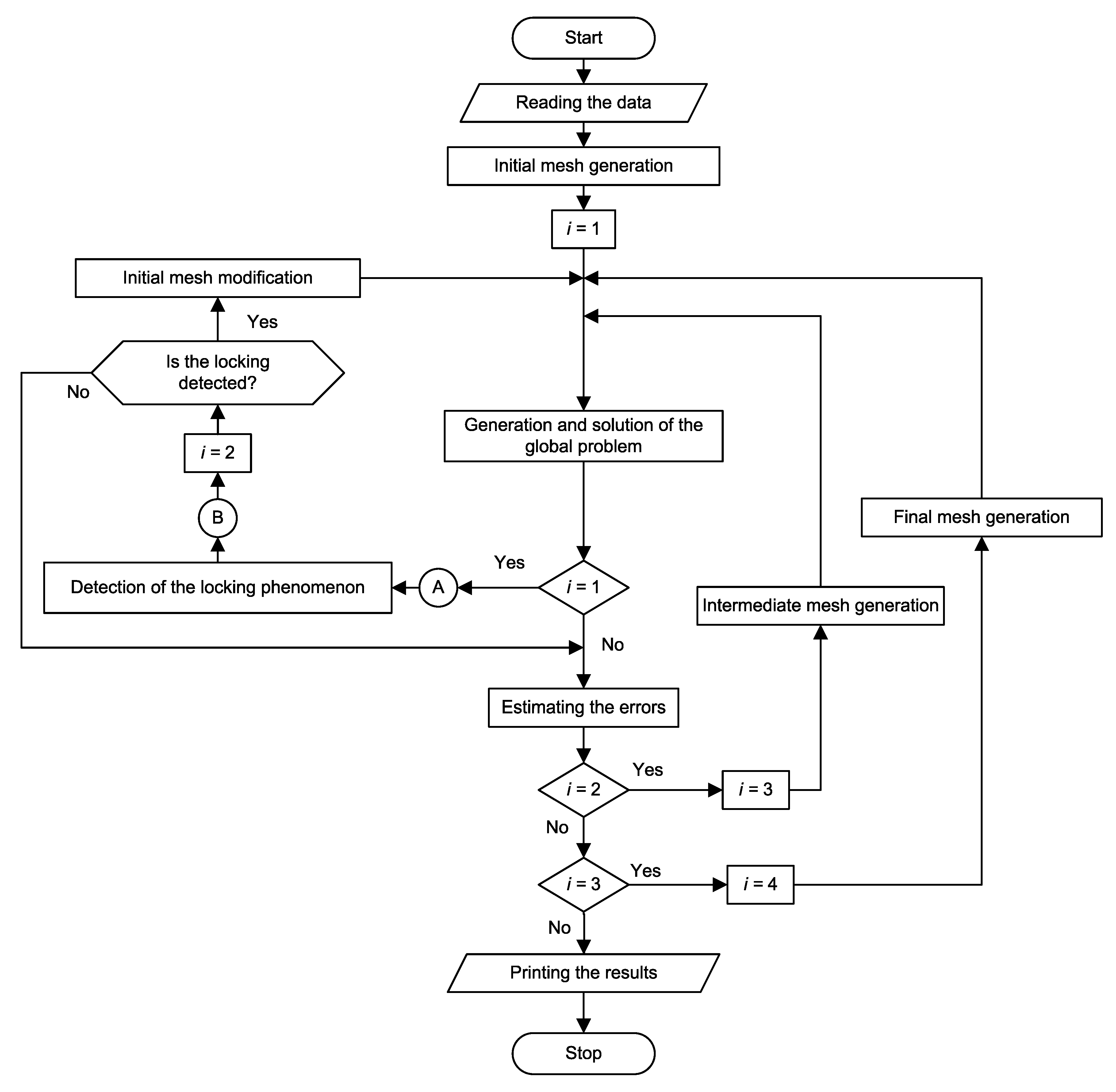
Figure 1. Three-step adaptive procedure extended with the fourth modification step.
Applsci 10 08247 g001
Figure 2. Flow diagram of the overall algorithm for the locking detection.
Applsci 10 08247 g002
Figure 3. The sum of local energies—the bending-dominated plate.
Applsci 10 08247 g003
Figure 4. The global energy—the bending-dominated plate.
Applsci 10 08247 g004
Figure 5. The sum of local energies—the bending-dominated shell.
Applsci 10 08247 g005
Figure 6. The global energy—the bending-dominated shell.
Applsci 10 08247 g006
Figure 7. The sum of local energies—the membrane-dominated shell.
Applsci 10 08247 g007
Figure 8. The global energy—the membrane-dominated shell.
Applsci 10 08247 g008
Figure 9. A quarter of a bending-dominated plate—initial mesh.
Applsci 10 08247 g009
Figure 10. A quarter of a bending-dominated plate—hp-adapted (final) mesh.
Applsci 10 08247 g010
Figure 11. A quarter of a bending-dominated plate—after simple detection, no hp-adaptation.
Applsci 10 08247 g011
Figure 12. A quarter of a bending-dominated plate—mesh after optimized modification.
Applsci 10 08247 g012
Figure 13. A quarter of a bending-dominated plate—after optimization and hp-adaptation.
Applsci 10 08247 g013
Figure 14. A quarter of a bending-dominated plate—convergence for three adaptation cases.
Applsci 10 08247 g014
Figure 15. A bending-dominated plate—initial mesh.
Applsci 10 08247 g015
Figure 16. A bending-dominated plate—hp-adapted (final) mesh.
Applsci 10 08247 g016
Figure 17. A bending-dominated plate—mesh after simple detection, no hp-adaptation.
Applsci 10 08247 g017
Figure 18. A bending-dominated plate—mesh after optimized modification.
Applsci 10 08247 g018
Figure 19. A bending-dominated plate—mesh after optimization and hp-adaptation.
Applsci 10 08247 g019
Figure 20. A bending-dominated plate—convergence for three adaptation cases.
Applsci 10 08247 g020
Figure 21. A quarter of a bending-dominated shell—initial mesh.
Applsci 10 08247 g021
Figure 22. A quarter of a bending-dominated shell—hp-adapted (final) mesh.
Applsci 10 08247 g022
Figure 23. A quarter of a bending-dominated shell—after simple detection and h-adaptation
Applsci 10 08247 g023
Figure 24. A quarter of a bending-dominated shell—mesh after optimized modification.
Applsci 10 08247 g024
Figure 25. A quarter of a bending-dominated shell—after optimization and hp-adaptation.
Applsci 10 08247 g025
Figure 26. A quarter of a bending-dominated shell—convergence for three adaptation cases.
Applsci 10 08247 g026
Figure 27. An octant of a membrane-dominated shell—initial mesh.
Applsci 10 08247 g027
Figure 28. An octant of a membrane-dominated shell—hp-adapted (final) mesh.
Applsci 10 08247 g028
Figure 29. An octant of a membrane-dominated shell—convergence for hp-adaptation.
Applsci 10 08247 g029
Table 1. Result summary—a quarter of the bending-dominated plate.
Adaptive MethodResult QuantityMesh Type
InitialModifiedIntermediateFinal
mesh figure no.Figure 9Figure 10
standarddofs number N [1]362259648
h p -adaptivitylog ( U r U ) [N/m] 0.459481 0.452821 2.352724
( U r U ) / U r [%] *99.998.40.15
mesh figure no.Figure 9Figure 11
standard h p dofs number N [1]36729
after detectionlog ( U r U ) [N/m]0.459481−1.43770
( U r U ) / U r [%] *99.91.27
mesh figure no.Figure 9Figure 12Figure 13
standard h p dofs number N [1]3653134387704
after optimizationlog ( U r U ) [N/m]0.459481−0.297250−1.531051−2.354113
( U r U ) / U r [%] *99.917.51.020.15
* admissible relative error value γ T = 1.0 %.
Table 2. Result summary—the bending-dominated plate.
Adaptive MethodResult QuantityMesh Type
InitialModifiedIntermediateFinal
mesh figure no.Figure 15Figure 16
standarddofs number N [1]362256381
h p -adaptivitylog ( U r U ) [N/m] 1.060969 1.059175 1.010223
( U r U ) / U r [%] *100.99.60.85
mesh figure no.Figure 15Figure 17
standard h p dofs number N [1]36729
after detectionlog ( U r U ) [N/m]1.060969−0.527871
( U r U ) / U r [%] *100.2.58
mesh figure no.Figure 15Figure 18Figure 19
standard h p dofs number N [1]3632452659279
after optimizationlog ( U r U ) [N/m]1.0609690.927962−0.817269−1.338752
( U r U ) / U r [%] *100.73.61.320.40
* admissible relative error value γ T = 2.0 %.
Table 3. Result summary—a quarter of the bending-dominated shell.
Adaptive MethodResult QuantityMesh Type
InitialModifiedIntermediateFinal
mesh figure no.Figure 21Figure 22
standarddofs number N [1]819188145
h p -adaptivitylog ( U r U ) [N/m] 8.015996 8.014184 6.184208
( U r U ) / U r [%] *99.999.51.47
mesh figure no.Figure 21Figure 23
standard h p dofs number N [1]817293294
after detectionlog ( U r U ) [N/m]8.0159966.3308425.930839
( U r U ) / U r [%] *99.92.060.82
mesh figure no.Figure 21Figure 24Figure 25
standard h p dofs number N [1]81324526510,512
after optimizationlog ( U r U ) [N/m]8.0159967.9787756.0391045.449802
( U r U ) / U r [%] *99.991.731.050.27
* admissible relative error value γ T = 0.7 %.
Table 4. Result summary—an octant of the membrane-dominated shell.
Adaptive MethodResult QuantityMesh Type
InitialModifiedIntermediateFinal
mesh figure no.Figure 27Figure 28
standarddofs number N [1]27306606
h p -adaptivitylog ( U r U ) [N/m] 3.017413 1.898823 0.086034
( U r U ) / U r [%] *16.91.290.02
* admissible relative error value γ T = 1.0 %.
Publisher’s Note: MDPI stays neutral with regard to jurisdictional claims in published maps and institutional affiliations.