Article

Environmental Impacts of Cement Production: A Statistical Analysis

by
Claudio Durastanti
1 and
Laura Moretti
2,*
1
Department of Basic and Applied Sciences for Engineering, Sapienza University of Rome, Via Antonio Scarpa 16, 00161 Rome, Italy
2
Department of Civil, Constructional and Environmental Engineering, Sapienza University of Rome, Via Eudossiana 18, 00184 Rome, Italy
*
Author to whom correspondence should be addressed.
Appl. Sci. 2020, 10(22), 8212; https://doi.org/10.3390/app10228212
Submission received: 6 November 2020 / Revised: 13 November 2020 / Accepted: 17 November 2020 / Published: 19 November 2020
(This article belongs to the Special Issue Sustainable and Durable Building Materials)

Abstract

:
The attention to environmental impacts of cement production has grown fast in recent decades. The cement industry is a significant greenhouse gases emitter mainly due to the calcinations of raw materials and the combustions of fuels. This paper investigates on the environmental performances of cement production and on the identification of factors driving emissions. For this purpose, a sample of 193 different recipes of gray cement produced in Italy from 2014 to 2019 according to the European standard EN 197-1. This paper identifies the consumption impact categories (e.g., fossil fuels, renewable and non-renewable secondary fuels) that explain the assessment of the Global Warming Potential, one of the most crucial impacts of cement production. Having regard to the overall examined dataset and each cement type, a set of predictive models is implemented and evaluated. A similar approach has been adopted to produce accurate predictive models for further environmental impact categories that quantify emissions to air. The obtained results provide important information that can support cement producers to develop low-impacting cement recipes.

1. Introduction

In recent years, the interest for environmental protection has grown faster, becoming an important criterion for public policy in social and political contexts [1,2]. The most pursued objective is to reduce emissions of greenhouse gases (e.g., carbon dioxide, nitrous oxide and methane), which are responsible for the greenhouse effect [3]. In particular, the cement industry contributes about 5% of global anthropogenic CO2 emissions excluding land-use change [4,5], as the production of the binder is a highly energy-intensive and emitting process. Calcination of raw materials for the cement production (e.g., limestone, clay, calcareous marl and other clay-like materials) and burning (fossil) fuels to maintain high temperature in the kiln are the processes with highest environmental impact. The former is a chemical emission, the latter a physical emission. Indeed, raw materials are heated inside large rotating furnaces at 1400 °C to form a solid substance called clinker [6]. During this process, chemical emissions mainly come from calcium carbonate (CaCO3) and magnesium carbonate (MgCO3) calcination according to Equations (1) and (2) [7,8]:
CaCO3(s) + heat → CaO(s) + CO2 (g)
MgCO3(s) + heat → MgO(s) + CO2 (g)
Clinker is then ground or milled with gypsum and other constituents (e.g., products, raw materials, additives, recycled waste) to produce cement [9]. According to [9], 5 main types of cement (CEM I to CEM V) and 27 products in the family of common cements are defined. They differ for composition (proportion by mass) of the main constituents, but all contain clinker. Therefore, its production affects the environmental performances of the final product and cannot be overlooked in this study. The chemical process described in Equations (1) and (2) implies more than 60% of total CO2 emissions due to clinker production, as confirmed by the mass balance published in the last Environmental Product Declaration (EPD) of the Italian cement production [10]. Chemical emissions are not reducible, but physical emissions resulting from fuel combustion for kiln firing can be managed and reduced using alternative/waste fuels [11] and/or by adopting energy-saving technologies [12]. However, these changes in production processes have to turn out in agreement with the required quality of the obtained products, related to construction or industrial uses [13], or with some special performances to obtain [14,15,16]. Moreover, in order to reduce the impacts of cement production, in the last decade the content of clinker in cement has decreased [17] using supplementary cementitious materials (e.g., gypsum, ground limestone, coal fly ash or blast furnace slag) [18,19,20]. Therefore, the cement industry is making efforts to reduce its environmental impacts in terms of greenhouse gases that reflect on other environmental performances. The standard EN 15804 “Sustainability of construction works, environmental product declarations, core rules for the product category of construction products” [21] defines the core rules for the product category of construction Products in order to assess the life cycle impact and develop a Type III environmental declaration (i.e., EPD) for any construction product and construction service [22].
According to [21], different parameters describe the environmental performances of a product, such as environmental impacts, resource use, waste categories, and output flows [23,24,25,26,27]. In the literature, several studies assessed the impacts of cement production considering its upstream processes (i.e., production of commodities, raw materials, transport to the factory plant, production process) [28]. The obtained results allow the cement industry to identify the best strategies to reduce its environmental impact. More in detail, the authors have Life Cycle Analysis (LCA) results of the Italian cement production from 2014 to 2019; this data refers to the environmental performances of one of the most important cement industries in Europe with over 19 million of Mg produced in 2019 [29]. The impacts of more than 190 cement powders produced according to [9] have been assessed with a “from cradle to gate” boundary approach using the database Ecoinvent 2.2 (Version 2.2, Ecoinvent, Zurich, Switzerland, 2007) and the software package SimaPro 8.0.5.13 (Version 8.0.5.13, Pré Consultants: Amersfoort, The Netherlands, 2016) [30]. 15 different impact categories were assessed to describe the characteristics of each cement powder recipe.
The goal of this work is to identify among these features the most relevant variables to predict the behavior of Global Warming Potential (GWP). To obtain these results, different models have been implemented, by means of linear regression and variable selection procedures, more specifically, the Akaike Information Criterion. Analogous models are developed also for the other impact categories that quantify emissions to air. A comparative analysis shows that the most important impact category to control GWP and other emissions is represented by the Abiotic depletion-fossil fuels (ADPf).

2. Data and Methods

After a quick introduction of the available dataset, this section provides the reader with the key concepts to investigate the behavior of the Global Warming Potential (GWP) and its connections with the production parameters, as well as a short summary of the statistical methods here employed.
The examined impact categories (ICs) comply with the standard EN 15804 [21]; Table 1 lists their name and units of measure.
ICs in Table 1 are available for a sample of 193 different recipes to produce 1 kg of gray cement, which can be classified into four types of cement (from CEM I to CEM IV according to [9]):
  • CEM I (i.e., Portland cement). It is the most impacting type because it contains at least 95% by mass of clinker and gypsum as minor additional constituent to control the “setting of cement”.
  • CEM II (i.e., Portland composite cement). It is composed of clinker with different proportion by mass (65–94%), main constituents (e.g., bastfurnace slag, silica fume, pozzolana, fly ash, burnt shale or limestone), and gypsum as minor additional constituent. In the examined panel, CEM II A-LL and CEM II-BLL (i.e., portland limestone cements) are taken into account. The former has 80–94% clinker, 6–20% limestone and 0–5% gypsum by mass, the latter has 65–79% clinker, 21–35% limestone and 0–5% gypsum by mass:
  • CEM III (i.e., blastfurnace cement) is composed of 35–64% clinker, 36–65% blastfurnace slag, 0–5% gypsum by mass; and
  • CEM IV (i.e., pozzolanic cement). It is composed of clinker and pozzolanic constituents (i.e., bastfurnace slag, silica fume, pozzolana, and fly ash). Two types of CEM IV are in the panel: CEM IV/A (65–89% clinker, 11–35% pozzolanic materials, 0–5% gypsum) and CEM IV/B (45–64% clinker, 11–35% pozzolanic materials, 0–5% gypsum).
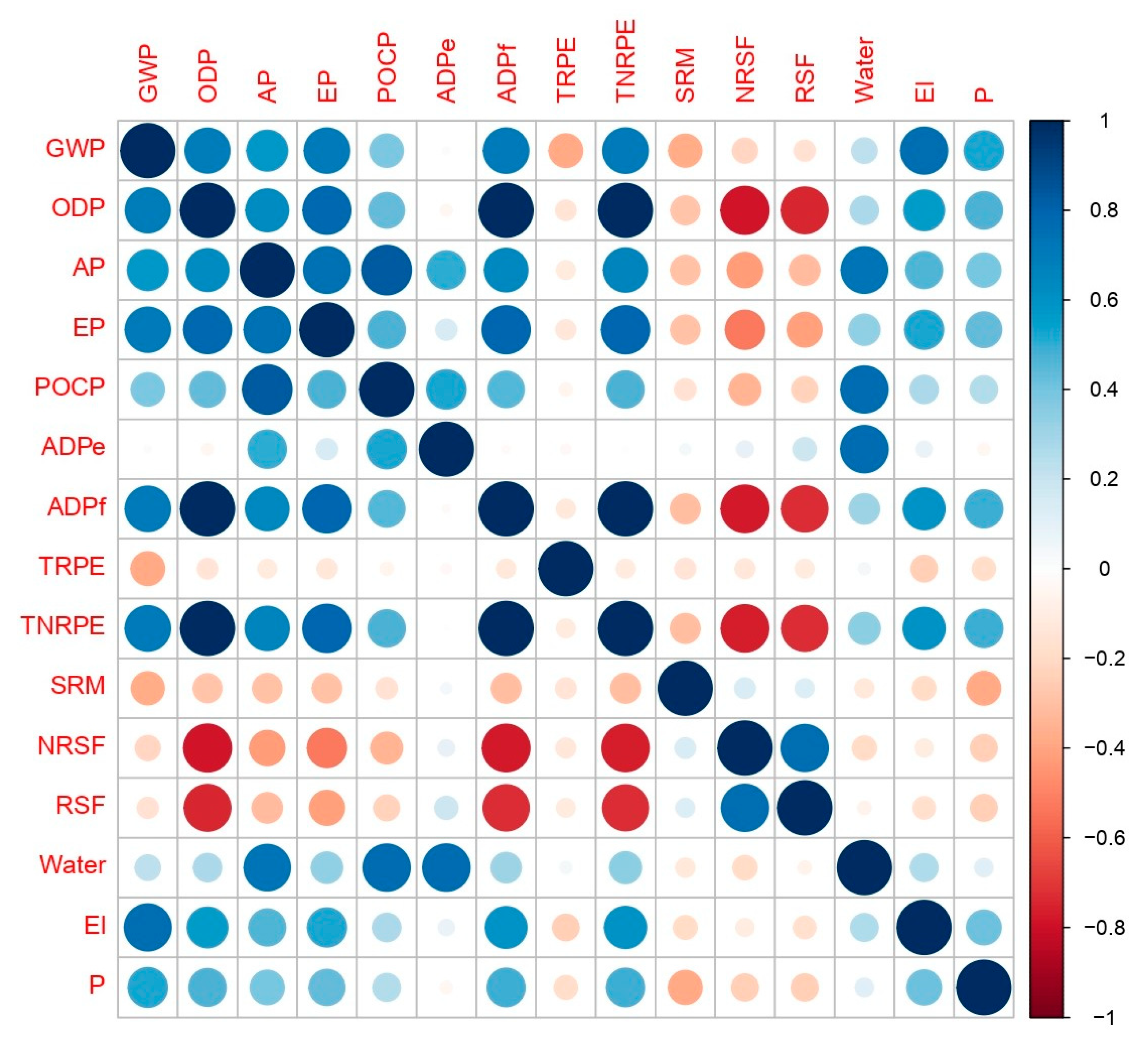
A preliminary analysis on the correlation matrix, performed to study relations between variables, is given in Figure 1. Positive and negative correlations are displayed in blue and red color, respectively, while the intensity of the color of each circle and its size is proportional to the absolute value of the corresponding correlation coefficient. Figure 1 shows that ODP, ADPf and TNRPE are pairwise perfectly correlated, that is, the corresponding correlation coefficient is equal to 1. This implies that these variables match deterministically, up to a multiplicative factor. For this reason, ODP and TNRPE are discarded in the further analysis. The remaining ICs have been used as independent variables and split into two groups, “Emissions” and “Consumption” (Table 2).
This work will focus on the following questions:
  • Which ones are the most relevant variables among the Consumption ICs in order to explain the behavior of GWP?
  • Are different variables important to predict GWP for the four types of cement?
  • Are the relevant variables to predict GWP also useful to predict other Emission ICs?
The answer to the first question is given by fitting and evaluating a linear regression model linking GWP to the Consumption ICs, (Equation (3)):
GWP = βADPe ADPe + βADPf ADPf + βTRPE TRPE + βSRM SRM + βnonRSF nonRSF + βRSF RSF + βWater Water + βEl El + ε
where ε is the so-called noise, a vector of size n = 193 of independent and identically distributed random variables, while (βADPe, βADPf, βTRPE, βSRM, βnonRSF, βRSF, βWater, βEl) is the vector of parameters to be estimated [31]. In statistics, linear regression is a widely used approach to establish the relationship between the so-called response (in our case GWP for Section 3.2 and Section 3.3, the other Emission ICs in Section 3.4) and a set of explanatory variables (here the Consumption ICs) [32]. The relationship between the response and the explanatory variables is modeled by means of a linear predictor function whose unknown model parameters are estimated from the data. In this work, all the linear models are fit by means of the so-called least squares approach, which minimizes the sum of the squared residuals (the differences between the observed value and the one predicted by the model. In our case, solving the regression problem produces a vector of estimators ( β ^ A D P e , β ^ A D P f , β ^ T R P E , β ^ S R M , β ^ n S R M , β ^ S R M , β ^ W a t e r , β ^ E l ) . The most relevant estimators can be then selected by means of the so-called Akaike Information Criterion (AIC) [32]. This procedure results in a model where only statistically significant variables in terms of the highest variances are selected, while the others are iteratively discarded. A model validation is then performed by means of a 10-fold cross validation procedure [31] to assess and compare the accuracy of the two models. Cross validation evaluates the accuracy of a predictive model, estimating its ability to predict new data. In the k-fold cross validation, the original dataset is randomly partitioned into k subsamples of equal size. Then, one subsample (the validation data) is used to test the model obtained by using the remaining k-1 subsamples (the so-called training data). This procedure is then repeated k times and averaged, so that all the observations are used for both validation and testing. The measure of the accuracy of each method is provided by the root mean square error, the risk function which measures the square root of the average squared difference between observations and the estimated values [31].
As far as the second question is concerned, it is now investigated if different types of cement influence GWP in different ways and, consequently, if the statistical model’s accuracy can be improved by fitting a separate regression model for each class. These regression models can be expressed as Equation (4):
GWP = βADPe;i ADPei + βADPf;i ADPfi + βTRPE;i TRPEi + βSRM;i SRMi + βnonRSF;i nonRSFi + βRSF;i RSFi + βWater;i Wateri + βEl;i Eli + εi
where i = I, II, III, IV and solving the regression model produces estimates for the set of parameters ( β A D P e ; i , β A D P f ; i , β T R P E ; i , β S R M ; i , β n o n R S F ; i , β W a t e r ; i , β E l ; i ) , i = I, …, IV. It is also relevant to check if some types of cement behave differently in terms of the regression models and relevant variables. Again, 10-fold cross validation procedures [31] are used to compare the results and to verify how accurate each predictive model is.
Regarding the third question, a multiple linear regression using the full set of Consumption ICs is performed and used to evaluate two alternative models. The first alternative model uses as input variables only the ones selected for GWP. The other alternative model develops different variables for each Emission IC, by means of the AIC criterion. If sufficiently accurate, the first model would allow the producer to focus on the same subset of variables to control jointly all the emissions. If it is not the case, the second model establishes which Consumption ICs are relevant to predict other emissions than GWP. Also in this case, a 10-fold cross validation procedure has been applied to compare the accuracy of the models. The statistical analysis has been performed within the R Cran environment [33] and the support of additional packages [34,35].

3. Results

In this section, details concerning the performed data analysis are presented and discussed to answer the questions introduced in Section 2. In particular, Section 3.1 includes some preliminary exploratory analysis. Section 3.2 concentrates on Question 1, by studying and comparing two models to predict GWP, the first model obtained by fitting a linear regression, and the second model by selecting the most relevant variables by means of the AIC criterion. Section 3.3 is concerned with Question 2. For each type of cement, a linear regression is fit and then the most important Consumption ICs are selected by the AIC criterion. Analogies and differences shown by the models here developed and the ones in Section 3.1 are then investigated. Section 3.4 is focused on the other Emission ICs and, then, on Question 3. For each type of Cement and for each Emission, three different models are studied and then compared. The first model is a linear regression which uses all the available Consumption ICs to predict each emission. The second model is a linear regression where only the relevant variables to GWP established in Section 3.2 are used. The third model selects the relevant variables for each Emission by the AIC criterion. The three models are then examined and compared to establish whether the same Consumption ICs can be used to predict accurately all the Emissions or not.

3.1. Exploratory Analysis

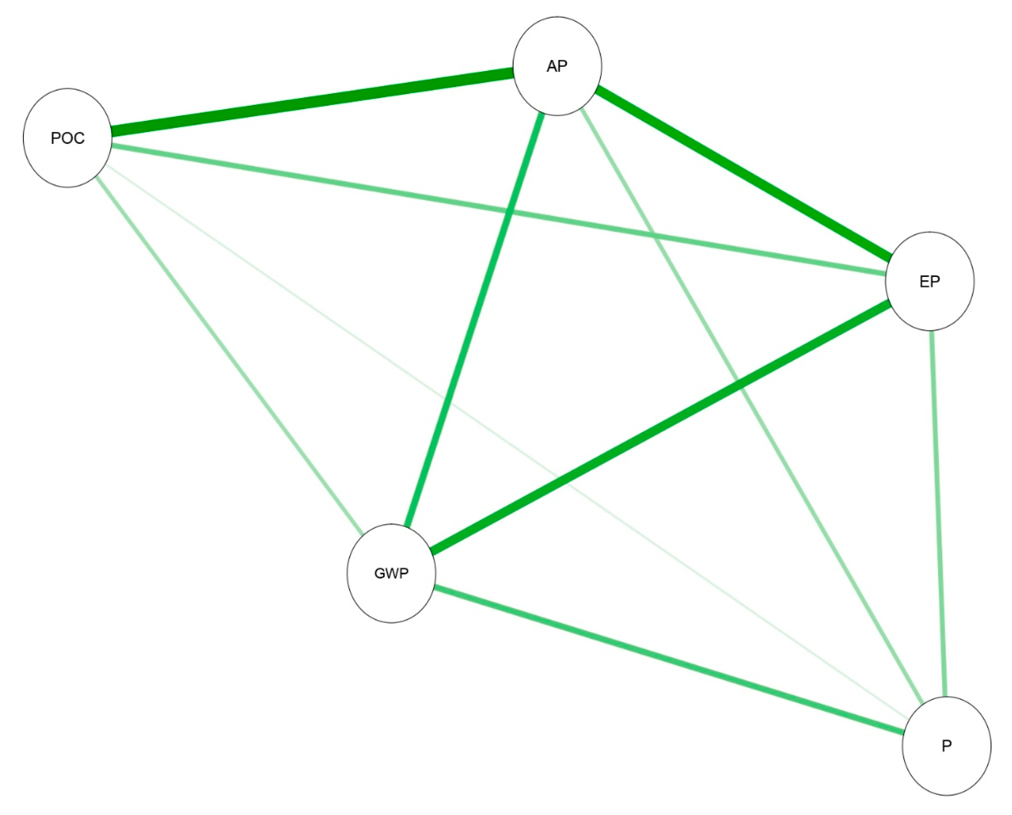
First, it is investigated if there is some relation linking GWP with the other Emission ICs, and it can be observed that all the Emission variables are positively correlated (i.e., green lines) with GWP, as shown in Table 3 and described in Figure 2.
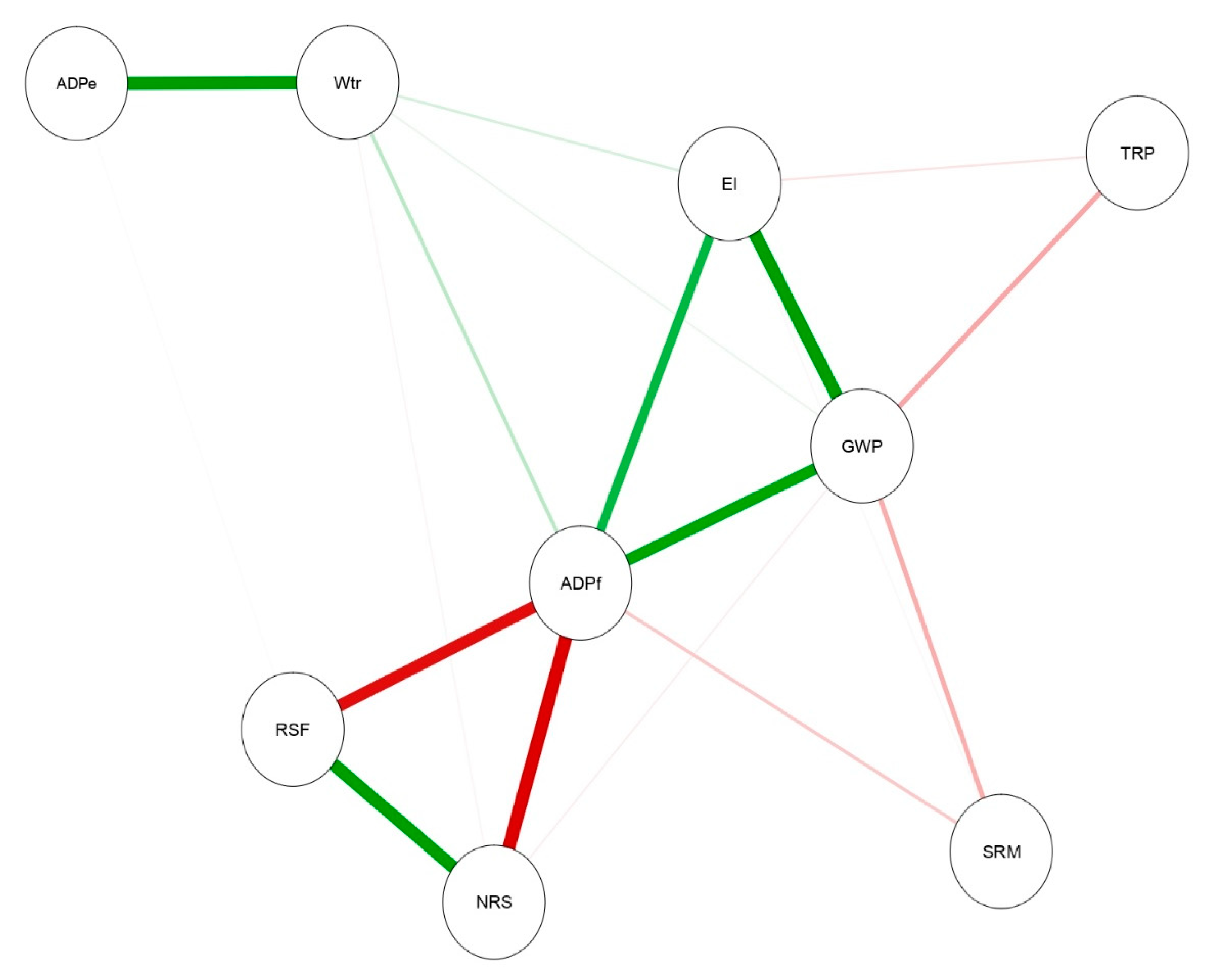
Table 4 presents the correlation coefficients of GWP with the Consumption variables, presented in Figure 4.
Having regard to the correlation coefficients, Figure 2 shows that all Emission ICs are positively correlated.
Figure 3 shows the correlation between GWP and the Consumption ICs. GWP is strongly positively correlated to ADPf and El and mildly negatively correlated to TRP and SRM. The results about GWP, El and ADPf comply with the physical meaning of these ICs. Indeed, the more fossil fuels and electricity are consumed, more greenhouse gases are emitted. On the other hand, the use of secondary fuels (both renewable and non-renewable) reduces the consumption of fossil fuels. Correlation between ADPe and water is due to the upstream processes (i.e., quarry extraction) of the cement production.
Therefore, the most relevant variables among the Consumption ICs that could explain the behavior of GWP are electricity and fossil fuels consumption. This complies with the Italian energy mix, whose main energy consumption is driven by petroleum and other liquids and natural gas [36]. On the other hand, the correlations between GWP and other Emission ICs (Table 3) and GWP and the Consumption ICs (Table 4) justify the international approach to protect the environment reducing greenhouse gas emissions. At this purpose, in 2003 the European Parliament and the Council established the Emissions Trading Scheme [37] to limit or reduce greenhouse gas emissions.
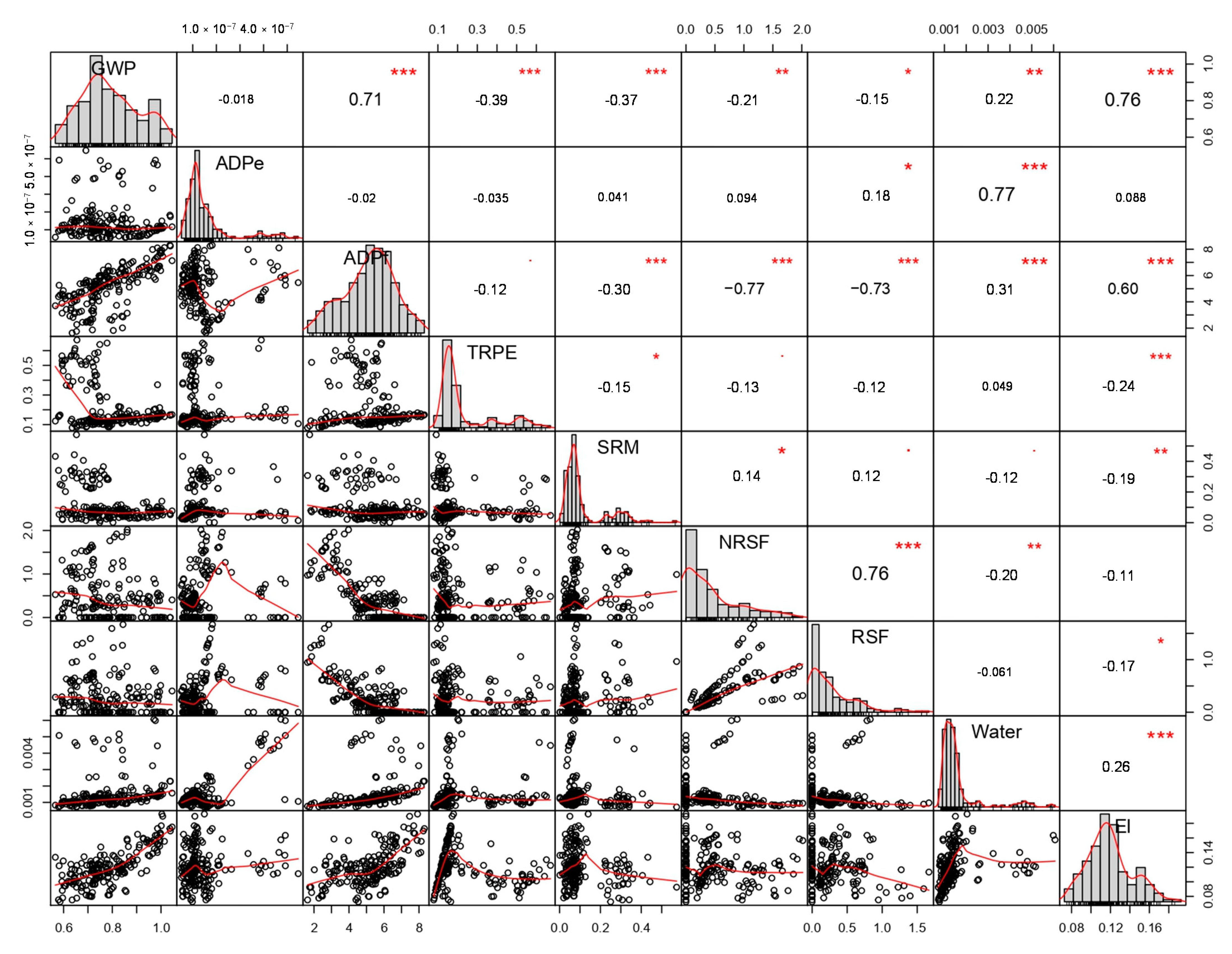
Figure 4 provides the reader with explicit correlation coefficients (in the top-right cells with respect to the main diagonal), an estimation of the density function by a histogram and a kernel density estimation (KDE) (in the main diagonal) and, finally, scatterplots with fitted nonparametric regression lines to stress the relationship between pairs of different variables (in the bottom-left cells with respect to the main diagonal). In the first column, each plot displays values for GWP paired with all the Consumption ICs, while in the first row the correlation coefficients between GWP and the Consumption ICs are listed.
In Figure 4 both x- and y- axis labels refer to the corresponding iCs listed in the main diagonal; their units comply with those listed in Table 1. Therefore, GWP values obtained in the LCA range between 0.6 and 1.0 kg CO2 eq./1 kg of produced cement; ADPe ranges between 1.0 × 10⁻⁷ and 5.0 × 10⁻⁷ kg Sb eq./1 kg of produced cement.

3.2. Linear Regression and Variable Selection for GWP

In this Section two predictive models for GWP are fit. The first model is a linear regression where GWP is the scalar response and the Consumption ICs are the input variables. All variables have been preliminarily normalized to simplify the interpretation. The estimated coefficients are listed in Table 5, together with the related standard deviations (St. dev.) and the corresponding significance for the p-values associated to the significance test of the model.
To develop the second model, an AIC backward selection procedure is then performed on the linear regression, to find the best subset of Consumption ICs to accurately predict GWP, leading to the model described in Table 6.
Then, a 10-fold cross-validation procedure is performed to compare the two models. The root mean square errors (RMSE) are computed by Equations (5) and (6):
R M S E l i n = ( 1 n i = 1 n ( G W P i β ^ A D P e l i n A D P e i β ^ A D P f l i n A D P f i β ^ T R P E l i n T R P E i β ^ S R M l i n S R M i β ^ N R S F l i n N R S F i β ^ R S F l i n R S F i β ^ W a t e r l i n W a t e r i β ^ E L l i n E L i ) 2 ) 1 / 2
R M S E A I C = ( 1 n i = 1 n ( G W P i β ^ A D P e A I C A D P e i β ^ A D P f A I C A D P f i β ^ T R P E A I C T R P E i β ^ S R M A I C S R M i β ^ N R S F A I C N R S F i β ^ R S F A I C R S F i β ^ W a t e r A I C W a t e r i β ^ E L A I C E L i ) 2 ) 1 / 2
for the linear and AIC model, respectively. The sample size n = 193 is the number of observations, while ( β ^ A D P e l i n , β ^ A D P f l i n , β ^ T R P E l i n , β ^ S R M l i n , β ^ N R S F l i n , β ^ R S F l i n , β ^ W a t e r l i n , β ^ E l i n ) , and ( β ^ A D P e A I C , β ^ A D P f A I C , β ^ T R P E A I C , β ^ S R M A I C , β ^ N R S F A I C , β ^ R S F A I C ) are the estimated parameters with the linear model and then selected by the AIC criterion, respectively. Recall that the RMSE is a risk function aimed to measure the discrepancy between the observations and the corresponding estimated values. In Table 7 R M S E l i n is higher than R M S E A I C , thus the variable reduction produces a more accurate model.
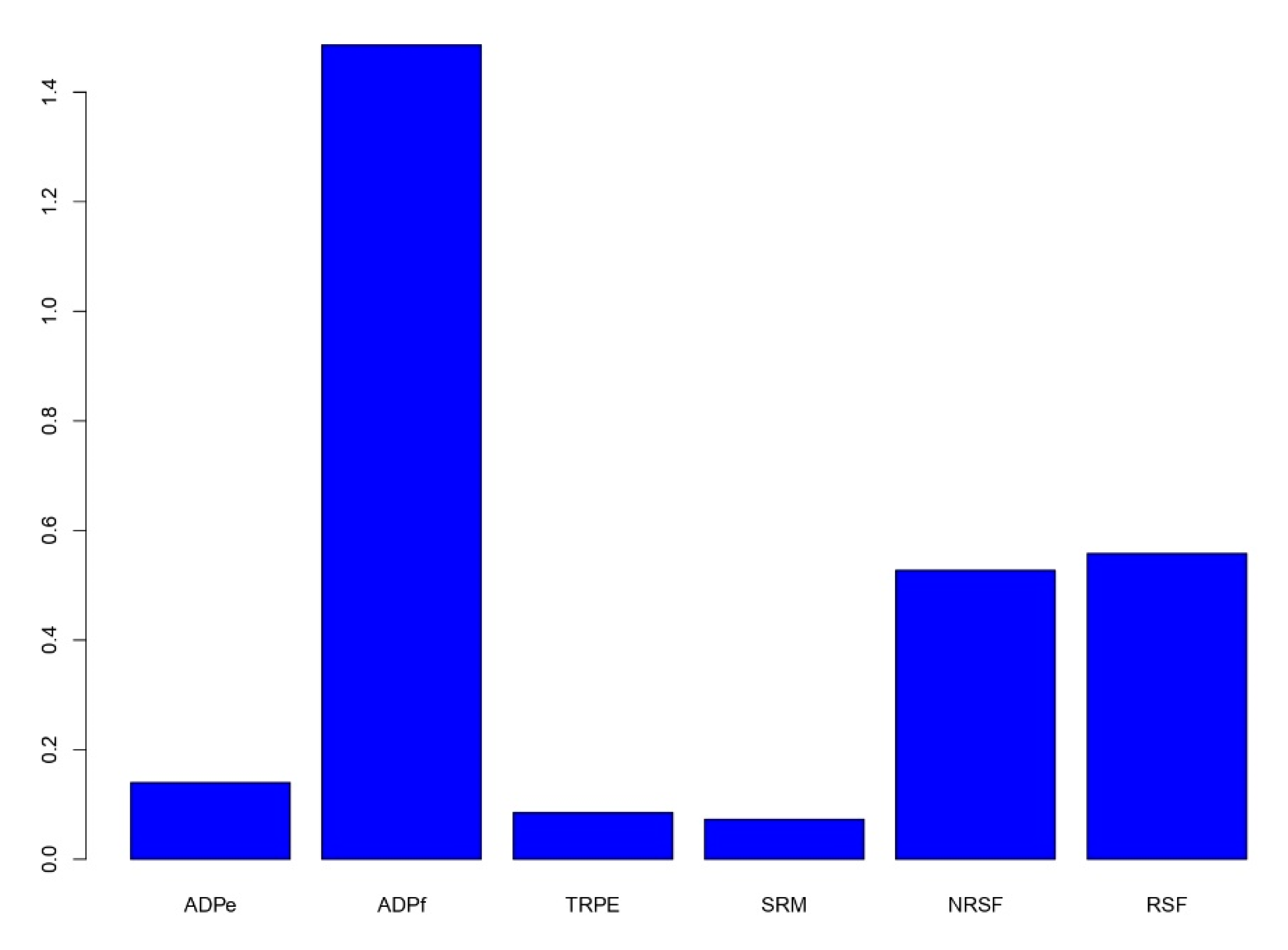
Finally, Figure 5 describes the size of each regression slope coefficient, after the variable selection. The highest contribution to GWP is given by ADPf. This result complies with the release of carbon dioxide into the atmosphere by burning of fossil fuels [38,39,40].
In answer to Question 1, the most relevant variables among the Consumption ICs to predict GWP are ADPf, NRSF and RSF. The energy-intensive industry of cement manufacturing can motivate this variable selection: all these ICs quantify the energy, mainly fossil but also alternative, spent in the process. This result complies with the efforts to implement in the cement sector different management systems, process-integrated techniques and end-of-pipe measures identified as Best Available Techniques (BAT) to have environmental benefits (e.g., thermal energy optimization techniques in the kiln system; reduction of electrical energy use; recovery of excess heat from the process and cogeneration of steam and electrical power) [41].

3.3. Linear Regression and Variable Selection for Each Type of Cement

The different types of cement are now studied separately to evaluate their impact on GWP. 
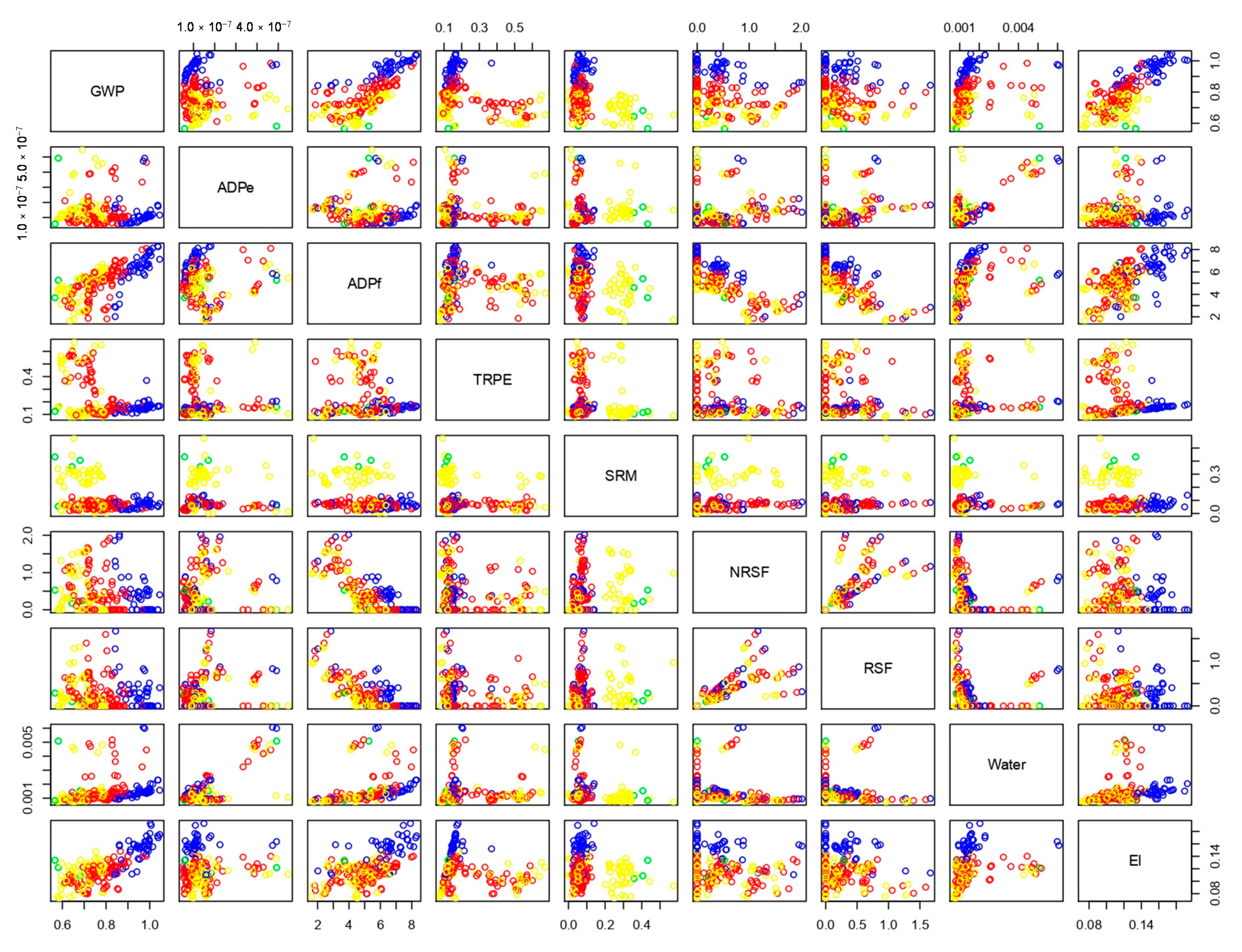
Figure 6, which contains the scatterplots related to GWP and the Consumption ICs, shows that the points associated to the class CEM I (in blue) are isolated in the GWP scatterplots with respect to the data belonging to the other types. Moreover, the environmental impacts of CEM I are higher than other investigated cement types: both the qualitative and the quantitative observed trends suggest investigating whether predictive models built separately for each class (type of cement) could achieve more accurate predictions for GWP. Furthermore, it is of extreme interest to check if different variables result to be important for each separate class with respect to the ones selected for the whole dataset. Figure 6 contains a matrix of scatterplots used to visualize the relationship between pairs of variables, all listed in the main diagonal. For each scatterplot, the variables in the x-axis (y-axis, respectively) can be found in the entry belonging to the main diagonal in the same column (row, respectively). The units of each axis label are listed in Table 1.
The dimensions of each class are given in Table 8.
Due to the small number of observations, CEM III is filtered out.
For each class, a linear regression is fit, where GWP corresponds to the scalar response and the ICs to the explanatory variables. The estimated regression coefficients for CEM I, II, and IV are listed in Table 9, Table 10 and Table 11, respectively.
Then, AIC backward selection procedures yield the models for the classes CEM I, II and IV described in Table 12, Table 13 and Table 14, respectively.
A 10-fold cross-validation procedure shows that the root mean square error (RMSE) related to the AIC selection model, is lower than the one computed for the full linear regression model (Table 15).
To answer to Question 2, also in this case a variable selection procedure leads to a more accurate model. Furthermore, different variables are selected as relevant depending on the type of cement. It can be observed that while for the class CEM I, the ICs TRPE and NRSF are discarded, for the classes CEM II and CEM IV the ones rejected by the AIC criterion are Water and El and the same ICs are selected. These ICs are also consistent also with the ones chosen for the whole dataset (except to SRM). The model for the class CEM I is characterized by a different set of variables and associated sizes, including Water and El (Figure 7 shows the size of the coefficients for each class and for the aggregate data, Figure 7a–d, respectively). It also confirms the qualitative interpretation of Figure 6, where data belonging to CEM I was mostly isolated.
The results of CEM I (Figure 7b) differ from CEM II and CEM IV (Figure 7c,d) due to its composition (i.e., at least 95% by mass of clinker and not more than 5% by mass of gypsum according to [9]), while other cement types contain less clinker and other main constituents.

3.4. Other Emission Variables

This section focuses on producing accurate models for the other Emission ICs. The first model here fit is a multiple linear regression model containing as target variables all the emissions. The results are collected in Table 16, Table 17 and Table 18 for CEM I, II and IV, respectively. Since in Section 3.3, subsampling data with respect to the type of cement has led to a more accurate model, also in this Section each type of cement is examined separately.
For each class, the second model consists in a linear model, which exploits only the variables established in Section 3.3 as relevant to predict GWP. The models are summarized in Table 19, Table 20 and Table 21 for CEM I, II, and IV, respectively.
A third model is finally produced applying the AIC criterion separately to each Emission IC for each class. Then, each of this model selects the most important variables for the corresponding IC. The results are summarized in the Table 22, Table 23 and Table 24 for CEM I, II, and IV, respectively.
A 10-fold cross-validation procedure shows that the root mean square error (RMSE) computed for AIC selection model built for each emission IC is lower than the one related to the full linear regression model and to the one associated to the variables selected to predict GWP. The two last RMSEs are among them comparable (Table 25).
In answer to Question 3, the results in Table 25 highlight that, while in general using the same subset of Consumption IC relevant to predict GWP does not improve the accuracy of the linear model, performing separately for each Emission IC a variable selection procedure leads to a meaningful enhancement in terms of predictive assessment of the model.
In Figure 8, all the important variables related to each Emission IC listed in Table 19, Table 20 and Table 21 are represented proportionally to their size.
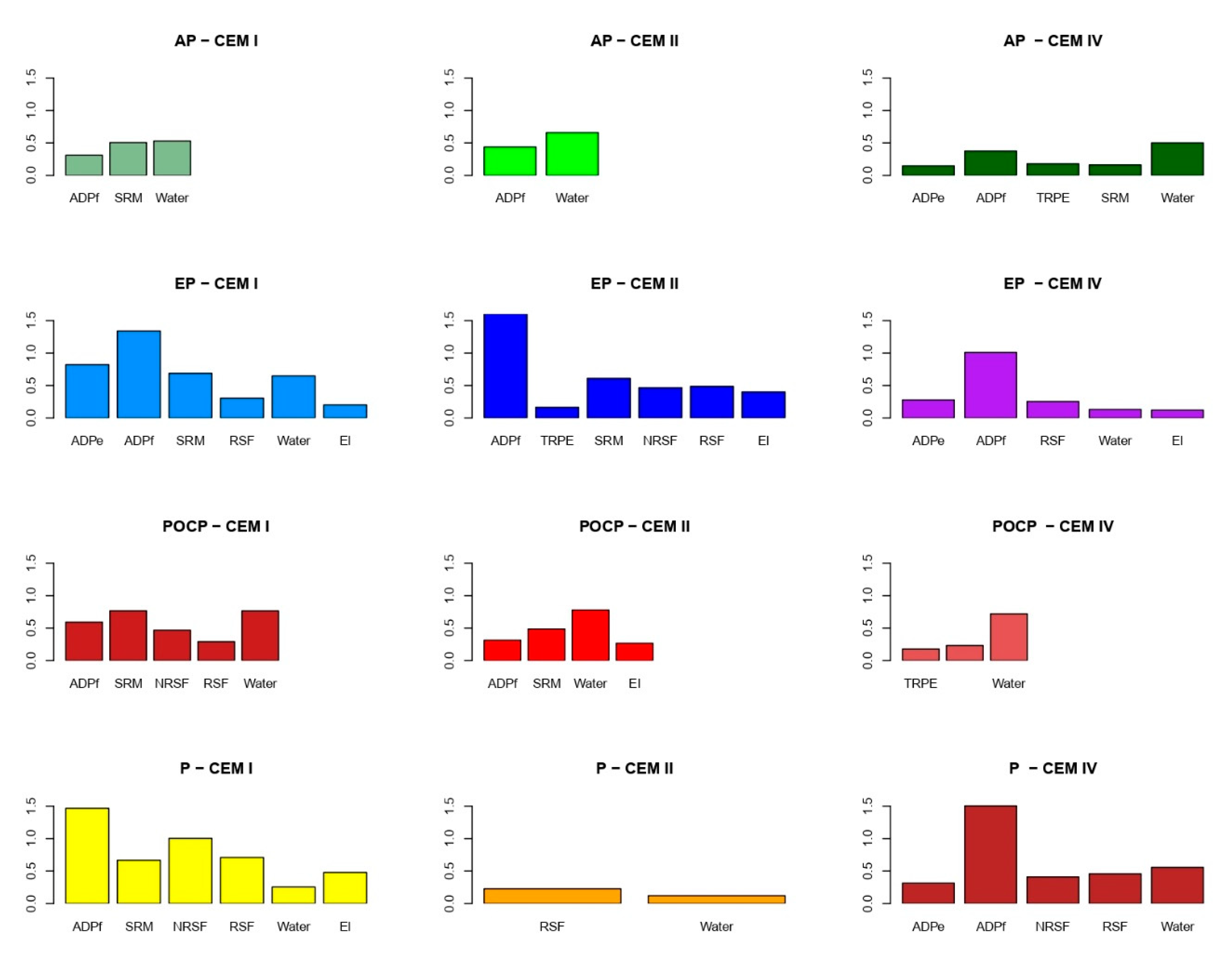
Figure 8 confirms that ADPf plays a pivotal role for the majority of IC emissions, that is, AP, EP, POCP and P (CEM I and CEM IV). CEM II differs from CEM I and CEM IV due to its limestone-based composition; particularly, POCP CEM II has its highest correlation with the Water consumption IC. It is confirmed by the upstream processes necessary to quarry natural raw materials.

4. Discussion

Due to a dependence on fossil fuels and the calcination of raw materials, the cement industry generates about 5% of global greenhouse gas emissions. Within this framework, several efforts are on-going to protect the environment and increase energy efficiency using renewable resources or alternative fuels. In order to analyze comparable environmental performances, cement companies are conducting life cycle assessment of their “from cradle to gate” processes in order to identify the best strategies to meet the need for sustainable development.
In this study, having regard to the European approach compliant with the standard EN 15804, the environmental impacts of 193 different recipes of gray cement produced in Italy from 2014 to 2019 have been assessed. Fifteen different impact categories have been considered and split into two classes, “Emissions” and “Consumption”. One of the main results of this work concerns the identification of the significant Consumption ICs to predict the behavior of Emission ICs, In particular, the target of this paper consists in answering to the following questions:
  • Which ones are the most relevant variables among the Consumption ICs in order to explain the behavior of GWP?
  • Are different variables important to predict GWP for the four types of cement?
  • Are the relevant variables to predict GWP also useful to predict other Emission ICs?
As far as Question 1 is concerned, it is shown that the most important variable to predict the behavior of GWP is ADPf (Figure 8), while NRSF and RSF are the two other most relevant consumption variables. To answer Question 2, a more accurate model is produced by fitting a linear regression and applying the AIC criterion for different types of cement (i.e., CEM I, CEM II, CEM IV) separately. Also in this case, ADPf is proved to be the most important Consumption IC. However, scatterplots related to GWP and the Consumption ICs show that the environmental performances of CEM I differ from those of the other types, and their values are higher. Predictive models built separately for each type of cement revealed more accurate predictions for GWP. Finally, concerning Question 3, the authors investigated if the relevant variables to predict GWP could predict other Emission ICs. In this case, it is shown that fitting separately regression models and selecting the most important variables leads to more accurate predictions for all the other Emissions ICs (Table 25) in comparison to the standard linear model or the one which uses the same Consumption ICs for GWP. Also in this case, ADPf is confirmed to be a strong predictor in the models related to the emission variables AP, EP, POCP (for CEM I and CEM II), and P (for CEM I and CEM IV). Therefore, the obtained results underline the need for policies and strategies that could reduce consumption of energy, both fossil and secondary fuels, and justify the European policies about Emission trading and Best Available Techniques to be implemented in the cement industry.

Author Contributions

Conceptualization, C.D. and L.M.; methodology, C.D.; software, C.D. and L.M.; validation, L.M. and C.D.; formal analysis, C.D.; data curation, L.M.; writing—original draft preparation, C.D. and L.M.; review and editing, C.D. and L.M. All authors have read and agreed to the published version of the manuscript.

Funding

This research received no external funding.

Conflicts of Interest

The authors declare no conflict of interest.

References

  1. Miccoli, S.; Finucci, F.; Murro, R. Assessing project quality: A multidimensional approach. Adv. Mater. Res. 2014, 1030–1032, 2519–2522. [Google Scholar] [CrossRef]
  2. Miccoli, S.; Finucci, F.; Murro, R. Criteria and procedures for regional environmental regeneration: A European strategic project. Appl. Mech. Mater. 2014, 675–677, 401–405. [Google Scholar] [CrossRef]
  3. Anderson, T.R.; Hawkins, E.; Jones, P.D. CO2, the greenhouse effect and global warming: From the pioneering work of Arrhenius and callendar to today’s Earth system models. Endeavour 2016, 40, 178–187. [Google Scholar] [CrossRef] [PubMed] [Green Version]
  4. Flower, D.J.M.; Sanjayan, J.G. Handbook of Low Carbon Concrete; Butterworth-Heinemann: Oxford, UK, 2017. [Google Scholar]
  5. Mahasenan, N.; Smith, S.; Humphreys, K. The cement industry and global climate change: Current and potential future cement industry CO2 emissions. Greenhouse gas control technologies. In Proceedings of the 6th International Conference on Greenhouse Gas Control Technologies, Kyoto, Japan, 1–4 October 2002. [Google Scholar]
  6. Gagg, C.R. Cement and concrete as an engineering material: An historic appraisal and case study analysis. Eng. Fail. Anal. 2014, 40, 114–140. [Google Scholar] [CrossRef]
  7. Olivier, J.G.J.; Peters, J.A.H.W.; Janssens-Maenhout, G. Trends in Global CO2 Emissions 2016 Report; PBL Netherlands Environmental Assessment Agency: The Hague, The Netherlands.
  8. Worrell, E.; Price, L.; Martin, N.; Hendriks, C.; Ozawa Meida, L. Carbon dioxide emissions from the global cement industry. Annu. Rev. Energy Environ. 2001, 26, 303–329. [Google Scholar] [CrossRef]
  9. European Committee for Standardization. EN 197-1: 2000, Cement—Part 1: Composition, Specifications and Conformity Criteria for Common Cements; European Committee for Standardization: Brussels, Belgium, 2000. [Google Scholar]
  10. AITEC. Dichiarazione Ambientale Cementi Grigi Medi Italia. Available online: https://gryphon4.environdec.com/system/data/files/6/18430/S-P-00880%20EPD%20(2020).pdf (accessed on 28 October 2020).
  11. Sonebi, M.; Ammar, Y.; Diederich, P. Sustainability of cement, concrete and cement replacement materials in construction. Sustain. Constr. Mater. 2016, 371–396. [Google Scholar] [CrossRef]
  12. Mokhtar, A.; Nasooti, M. A decision support tool for cement industry to select energy efficiency measures. Energy Strategy Rev. 2020, 28, 100458. [Google Scholar] [CrossRef]
  13. Loprencipe, G.; Cantisani, G. Evaluation methods for improving surface geometry of concrete floors: A case study. Case Stud. Struct. Eng. 2015, 4, 14–25. [Google Scholar] [CrossRef] [Green Version]
  14. Cantisani, G.; D’Andrea, A.; Moretti, L. Natural lighting of road pre-tunnels: A methodology to assess the luminance on the pavement—Part, I. Tunn. Undergr. Space Technol. 2018, 73, 37–47. [Google Scholar] [CrossRef]
  15. Cantisani, G.; D’Andrea, A.; Moretti, L. Natural lighting of road pre-tunnels: A methodology to assess the luminance on the pavement—Part II. Tunn. Undergr. Space Technol. 2018, 73, 170–178. [Google Scholar] [CrossRef]
  16. Loprencipe, G.; Cantisani, G.; Di Mascio, P. Global assessment method of road distresses. Life-Cycle of Structural Systems: Design, Assessment, Maintenance and Management. In Proceedings of the 4th International Symposium on Life-Cycle Civil Engineering (IALCCE) 2014, Tokyo, Japan, 16–19 November 2014; pp. 1113–1120. [Google Scholar]
  17. PBL Netherlands Environmental Assessment Agency. Trends in Global CO2 Emissions: 2012 Report. Available online: https://ec.europa.eu/jrc/en/publication/eur-scientific-and-technical-research-reports/trends-global-co2-emissions-2012-report (accessed on 28 October 2020).
  18. Mohammadi, J.; South, W. Effect of up to 12% substitution of clinker with limestone on commercial grade concrete containing supplementary cementitious materials. Constr. Build. Mat. 2016, 115, 555–564. [Google Scholar] [CrossRef]
  19. Staněk, T.; Sulovský, P.; Boháč, M. Berlinite substitution in the cement clinker. Cem. Concr. Res. 2017, 92, 21–28. [Google Scholar] [CrossRef]
  20. Halbiniak, J.; Katzer, J.; Major, M.; Major, I. A Proposition of an in situ production of a blended cement. Materials 2020, 13, 2289. [Google Scholar] [CrossRef] [PubMed]
  21. European Committee for Standardization. EN 15804:2012+A1:2013. Sustainability of Construction Works—Environmental Product Declarations—Core Rules for the Product Category of Construction Products; European Committee for Standardization: Brussels, Belgium, 2013. [Google Scholar]
  22. International Organization for Standardization (ISO). ISO 14025:2006. Environmental Labels and Declarations—Type III Environmental Declarations—Principles and Procedures; International Organization for Standardization (ISO): Geneva, Switzerland, 2006. [Google Scholar]
  23. Stafford, F.N.; Raupp-Pereira, F.; Labrincha, J.A.; Hotza, D. Life cycle assessment of the production of cement: A Brazilian case study. J. Clean. Prod. 2016, 137, 1293–1299. [Google Scholar] [CrossRef]
  24. Moretti, L.; Caro, S. Critical analysis of the life cycle assessment of the Italian cement industry. J. Clean. Prod. 2017, 152, 198–210. [Google Scholar] [CrossRef]
  25. Rosyid, A.; Boedisantoso, R.; Iswara, A.P. Environmental impact studied using life cycle assessment on cement industry. IOP Conf. Ser. Earth Environ. Sci. 2020, 506, 012024. [Google Scholar] [CrossRef]
  26. Tun, T.Z.; Bonnet, S.; Gheewala, S.H. Life cycle assessment of Portland cement production in Myanmar. Int. J. Life Cycle Assess. 2020, in press. [Google Scholar] [CrossRef]
  27. Song, D.; Lin, L.; Wu, Y. Extended exergy accounting for a typical cement industry in China. Energy 2019, 174, 678–686. [Google Scholar] [CrossRef]
  28. Vázquez-Rowe, I.; Ziegler-Rodriguez, K.; Laso, J.; Quispe, I.; Aldaco, R.; Kahhat, R. Production of cement in Peru: Understanding carbon-related environmental impacts and their policy implications. Resour. Conserv. Recycl. 2019, 142, 283–292. [Google Scholar] [CrossRef]
  29. Federbeton. Rapporto di Filiera. 2019. Available online: https://www.aitecweb.com/Portals/0/pubdoc/pubblicazioni/Rapporti/Federbeton_Rapporto_di_Filiera_2019.pdf (accessed on 29 October 2020).
  30. SimaPro 8.0.5.13; Software SimaPro. Pré; Consultants: Amersfoort, The Netherlands, 2016.
  31. Wasserman, L. All of Statistics: A Concise Course on Statistical Inference; Springer: Cham, Switzerland, 2013. [Google Scholar]
  32. Giraud, C. Introduction to High-Dimensional Statistics; CRC Press: Boca Raton, FL, USA, 2015. [Google Scholar]
  33. R Core Team. A Language and Environment for Statistical Computing; R Foundation for Statistical Computing: Vienna, Austria, 2017. [Google Scholar]
  34. Peterson, B.G.; Carl, P. PerformanceAnalytics: Econometric Tools for Performance and Risk Analysis. R Package Version 2.0.4. Available online: https://CRAN.R-project.org/package=PerformanceAnalytics (accessed on 18 November 2020).
  35. Jackson, S. Corrr R: Correlations in R. R Package. 2016. Available online: https://github.com/drsimonj/corrr (accessed on 18 November 2020).
  36. Cantisani, G.; Moretti, L.; Carrarini, L.; Bezzi, F.; Cherubini, V.; Nicotra, S. Italian road tunnels: Economical and environmental effects of an on-going project to reduce lighting consumption. Sustainability 2019, 11, 4631. [Google Scholar]
  37. European Union. Directive 2003/87/EC of the European Parliament and the Council of 13 October 2003 Establishing a Scheme for Greenhouse Gas Emission Allowance Trading within the Community and Amending Council Directive 96/61/EC.; European Union: Brussels, Belgium, 2003. [Google Scholar]
  38. Chen, K.; Winterb, R.C.; Bergman, M.K. Carbon dioxide from fossil fuels: Adapting to uncertainty. Energy Policy 1980, 8, 318–330. [Google Scholar] [CrossRef] [Green Version]
  39. von Hippel, D.; Raskin, P.; Subak, S.; Stavisky, D. Estimating greenhouse gas emissions from fossil fuel consumption Two approaches compared. Energy Policy 1993, 21, 691–702. [Google Scholar] [CrossRef]
  40. Shurpali, N.; Agarwal, A.K.; Srivastava, V.K. Greenhouse Gas. Emissions. Challenges, Technologies and Solutions; Springer: Singapore, 2019; ISBN 978-981-13-3271-5. [Google Scholar]
  41. European Commission. Best Available Techniques (BAT) Reference Document for the Production of Cement, Lime and Magnesium Oxide: Industrial Emissions Directive 2010/75/EU (Integrated Pollution Prevention and Control.); European Commission: Brussels, Belgium, 2013. [Google Scholar]
Figure 1. Correlation matrix of ICs.
Applsci 10 08212 g001
Figure 2. Correlation among Emission ICs.
Applsci 10 08212 g002
Figure 3. Correlation between GWP and the Consumption ICs.
Applsci 10 08212 g003
Figure 4. Correlation matrix analysis (GWP vs. Consumption ICs). “***” (p-value ≤ 0.001), “**” (p-value ≤ 0.01), “*” (p-value ≤ 0.05), “.” (p-value ≤ 0.1), and “ ” otherwise. This notation is valid throughout the article.
Applsci 10 08212 g004
Figure 5. Size of the coefficients (AIC selected components—absolute values).
Applsci 10 08212 g005
Figure 6. Data and types of cement. (CEM I = blue, CEM II = red, CEM III = green, CEM IV = yellow).
Applsci 10 08212 g006
Figure 7. Size of the coefficients (AIC selected components) for each type of cement (absolute values). (a) aggregated data; (b) CEM I; (c) CEM II; (d) CEM IV.
Applsci 10 08212 g007
Figure 8. Size of the coefficients (AIC selected components) for each class and for all the remaining Emission ICs. (absolute values).
Applsci 10 08212 g008
Table 1. Assessed impact categories.
Impact CategoryICUnit
Global Warming PotentialGWPkg CO2 eq
Ozone layer Depletion PotentialODPkg CFC-11 eq
Acidification PotentialAPkg SO2 eq
Eutrophication PotentialEPkg PO4 eq
Photochemical oxidation PotentialPOCPkg C2H4 eq
Abiotic depletion-elementsADPekg Sb eq
Abiotic depletion-fossil fuelsADPfMJ
Total Use of Renewable Primary Energy TRPEMJ
Total Use of non-Renewable Primary energyTNRPEMJ
Use of secondary raw materialsSRMkg
Non-renewable secondary fuelsnonRSFMJ
Renewable secondary fuelsRSFMJ
Water depletionWaterm3
ElectricityElkWh
ParticulatesPkg PTS
Table 2. Classes of ICs.
EmissionConsumption
GWP, AP, EP, POCP, PADPe, ADPf, TRPE, SRM, nonRSF, RSF, Water, El
Table 3. Correlation of GWP with Emission ICs.
ICAPEPPOCPP
Correlation coefficients0.5750.7030.3810.529
Table 4. Correlation of GWP with Consumption ICs.
ICADPeADPfTRPESRMNRSFRSFWaterEl
Correlation coefficients−0.0180.706−0.387−0.372−0.213−0.1520.2210.757
Table 5. Linear regression summary (GWP vs. Consumption ICs).
ICsLinear Regression (GWP vs. Consumption ICs)
CoefficientsSt. Dev.p-Value
ADPe−0.1270.038**
ADPf1.5030.077***
TRPE−0.0820.026**
SRM0.5320.025**
NRSF0.5310.052***
RSF0.5630.039***
Water−0.0170.041
El−0.0060.043
“***” (p-value ≤ 0.001), “**” (p-value ≤ 0.01) and “ ” otherwise.
Table 6. Linear regression model summary (after variable selection).
ICsLinear Regression (GWP vs. Selected Consumption ICs)
CoefficientsSt. Dev.p-Value
ADPe−0.1400.022***
ADPf1.4860.044***
TRPE−0.0850.025***
SRM0.5270.024**
NRSF0.5270.040***
RSF0.5580.037***
“***” (p-value ≤ 0.001), “**” (p-value ≤ 0.01).
Table 7. Comparison of RMSE between the two models.
ModelRMSE
Linear0.313
AIC0.305
Table 8. Dimensions of datasets related to each type of cement.
Cement TypeDimension of Classes
CEM I44
CEM II84
CEM III4
CEM IV61
Table 9. Linear regression summary (GWP vs. Consumption ICs)—CEM I.
ICsLinear Regression (GWP vs. Consumption ICs) CEM I
CoefficientsSt. Dev.p-Value
ADPe0.2170.115
ADPf0.7010.128***
TRPE0.1050.115
SRM0.0460.111
NRSF0.0900.079
RSF0.1810.061**
Water−0.1650.092.
El0.0520.050
“***” (p-value ≤ 0.001), “**” (p-value ≤ 0.01), “.” (p-value ≤ 0.1), and “ ” otherwise.
Table 10. Linear regression summary (GWP vs. Consumption ICs)—CEM II.
ICsLinear Regression (GWP vs. Consumption ICs) CEM II
CoefficientsSt. Dev.p-Value
ADPe−0.0520.099
ADPf1.2370.156***
TRPE−0.1320.044**
SRM0.0520.148
NRSF0.3890.104***
RSF0.4140.077***
Water−0.0290.089
El−0.0520.081
“***” (p-value ≤ 0.001), “**” (p-value ≤ 0.01) and “ ” otherwise.
Table 11. Linear regression summary (GWP vs. Consumption ICs)—CEM IV.
ICsLinear Regression (GWP vs. Consumption ICs) CEM IV
CoefficientsSt. Dev.p-Value
ADPe−0.0490.045
ADPf1.2340.157***
TRPE−0.0950.037*
SRM−0.0070.032
NRSF0.4200.091***
RSF0.4120.082***
Water−0.0160.062
El−0.0380.064
“***” (p-value ≤ 0.001), “*” (p-value ≤ 0.05), and “ ” otherwise.
Table 12. AIC selection model (GWP vs. Consumption ICs)—CEM I.
ICsLinear Regression (GWP vs. Consumption ICs) CEM I
CoefficientsSt. Dev.p-Value
ADPe0.2670.103*
ADPf0.5980.069***
RSF0.1630.053**
Water−0.1900.085*
El0.0940.041*
“***” (p-value ≤ 0.001), “**” (p-value ≤ 0.01), “*” (p-value ≤ 0.05).
Table 13. AIC selection model (GWP vs. Consumption ICs)—CEM II.
ICsLinear Regression (GWP vs. Consumption ICs) CEM II
CoefficientsSt. Dev.p-Value
ADPe−0.0820.043.
ADPf1.180.117***
TRPE−0.1330.042**
NRSF0.3640.075***
RSF0.4090.072***
“***” (p-value ≤ 0.001), “**” (p-value ≤ 0.01), “.” (p-value ≤ 0.1).
Table 14. AIC selection model (GWP vs. Consumption ICs)—CEM IV.
ICsLinear Regression (GWP vs. Consumption ICs) CEM IV
CoefficientsSt. Dev.p-Value
ADPe−0.0570.059
ADPf1.1730.035***
TRPE−0.1000.114**
NRSF0.3870.073***
RSF0.3940.075***
“***” (p-value ≤ 0.001), “**” (p-value ≤ 0.01), and “ ” otherwise.
Table 15. Comparison of RMSE between the two models.
ModelRMSE
linear0.275
AIC0.266
Table 16. Linear regression summary—CEM I.
ICsLinear Regression (AP vs. Consumption ICs) CEM I
CoefficientsSt. Dev.p-Value
ADPe0.1990.314
ADPf0.1840.349
TRPE0.4240.313
SRM0.4240.302
NRSF−0.1480.217
RSF−0.0570.166
Water0.3800.251
El−0.0700.135
ICsLinear Regression (EP vs. Consumption ICs) CEM I
CoefficientsSt. Dev.p-Value
ADPe0.7440.409
ADPf1.5710.454**
TRPE0.0850.408
SRM0.7320.394.
NRSF0.1870.283
RSF0.3550.216
Water−0.6150.327.
El−0.2730.176
ICsLinear Regression (POCP vs. Consumption ICs) CEM I
CoefficientsSt. Dev.p-Value
ADPe−0.0340.427
ADPf−0.5670.474
TRPE0.3640.425
SRM0.7980.410.
NRSF−0.4400.295
RSF−0.3140.226
Water0.7860.341*
El−0.1050.183
ICsLinear Regression (P vs. Consumption ICs) CEM I
CoefficientsSt. Dev.p-Value
ADPe−0.3410.471
ADPf−1.3250.523*
TRPE−0.5140.469
SRM−0.5040.453
NRSF−0.8730.325*
RSF−0.5900.249*
Water0.5140.376
El0.5200.203*
“**” (p-value ≤ 0.01), “*” (p-value ≤ 0.05), “.” (p-value ≤ 0.1), and “ ” otherwise.
Table 17. Linear regression summary—CEM II.
ICsLinear Regression (AP vs. Consumption ICs) CEM II
CoefficientsSt. Dev.p-Value
ADPe0.0670.180
ADPf0.6380.284*
TRPE−0.0030.079
SRM0.1750.269
NRSF0.1160.189
RSF0.0170.140
Water0.6050.160***
El−0.1600.147
ICsLinear Regression (EP vs. Consumption ICs) CEM II
CoefficientsSt. Dev.p-Value
ADPe0.0840.187
ADPf1.7090.296***
TRPE0.1450.083.
SRM0.6270.281*
NRSF0.4110.197*
RSF0.4270.146**
Water−0.0250.168
El−0.3940.153*
ICsLinear Regression (POCP vs. Consumption ICs) CEM II
CoefficientsSt. Dev.p-Value
ADPe−0.1780.199
ADPf−0.2890.314
TRPE−0.0330.088
SRM0.4950.298.
NRSF0.0940.209
RSF−0.0650.155
Water0.9500.178***
El−0.2960.162.
ICsLinear Regression (P vs. Consumption ICs) CEM II
CoefficientsSt. Dev.p-Value
ADPe−0.0100.249
ADPf−0.0450.393
TRPE−0.0840.110
SRM−0.0220.372
NRSF0.0220.261
RSF−0.2870.193
Water0.1410.222
El−0.0280.203
“***” (p-value ≤ 0.001), “**” (p-value ≤ 0.01), “*” (p-value ≤ 0.05), “.” (p-value ≤ 0.1), and “ ” otherwise.
Table 18. Linear regression summary—CEM IV
ICsLinear Regression (AP vs. Consumption ICs) CEM IV
CoefficientsSt. Dev.p-Value
ADPe0.1990.314*
ADPf0.1850.349
TRPE0.4240.313
SRM0.4240.302
NRSF−0.1480.217
RSF−0.0570.166
Water0.3800.251
El−0.0700.135
ICsLinear Regression (EP vs. Consumption ICs) CEM IV
CoefficientsSt. Dev.p-Value
ADPe0.7440.409.
ADPf1.5710.454**
TRPE0.0840.408
SRM0.7320.394.
NRSF0.1870.283
RSF0.3550.216
Water−0.6150.327.
El−0.2730.176
ICsLinear Regression (POCP vs. Consumption ICs) CEM IV
CoefficientsSt. Dev.p-Value
ADPe−0.0330.427
ADPf−0.5680.474
TRPE0.3640.425
SRM0.7980.411
NRSF−0.4400.295.
RSF−0.3140.226
Water0.7850.341*
El−0.1050.184
ICsLinear Regression (P vs. Consumption ICs) CEM IV
CoefficientsSt. Dev.p-Value
ADPe−0.3400.471
ADPf−1.3250.523*
TRPE−0.5140.470
SRM−0.5050.453
NRSF−0.8730.326*
RSF−0.5890.249*
Water0.5140.376
El0.5200.202*
“**” (p-value ≤ 0.01), “*” (p-value ≤ 0.05), “.” (p-value ≤ 0.1), and “ ” otherwise.
Table 19. AIC selection for GWP regression summary—CEM I.
ICsLinear Regression (AP vs. Consumption ICs) CEM I
CoefficientsSt. Dev.p-Value
ADPe0.3400.288
ADPf0.4780.191*
RSF0.0310.148
Water0.2620.237
El−0.0510.115
ICsLinear Regression (EP vs. Consumption ICs) CEM I
CoefficientsSt. Dev.p-Value
ADPe1.0800.370**
ADPf1.4110.247***
RSF0.3020.190
Water−0.8500.306**
El−0.1700.149
ICsLinear Regression (POCP vs. Consumption ICs) CEM I
CoefficientsSt. Dev.p-Value
ADPe0.1580.407
ADPf0.1470.270
RSF−0.1490.209
Water0.5880.335.
El−0.1670.163
ICsLinear Regression (P vs. Consumption ICs) CEM I
CoefficientsSt. Dev.p-Value
ADPe−0.8160.462
ADPf−0.2780.307.
RSF−0.3650.237
Water0.7590.381.
El0.1640.186
“***” (p-value ≤ 0.001), “**” (p-value ≤ 0.01), “*” (p-value ≤ 0.05), “.” (p-value ≤ 0.1), and “ ” otherwise.
Table 20. AIC selection for GWP regression summary—CEM II.
ICsLinear Regression (AP vs. Consumption ICs) CEM II
CoefficientsSt. Dev.p-Value
ADPe0.6710.084
ADPf0.3680.231***
TRPE−0.0410.083
NRSF−0.2050.147
RSF−0.0980.142
ICsLinear Regression (EP vs. Consumption ICs) CEM II
CoefficientsSt. Dev.p-Value
ADPe0.0550.085
ADPf1.2720.235***
TRPE0.1300.084
NRSF0.1730.150
RSF0.3720.145*
ICsLinear Regression (POCP vs. Consumption ICs) CEM II
CoefficientsSt. Dev.p-Value
ADPe0.7660.101
ADPf−0.1760.278***
TRPE−0.0910.100
NRSF−0.4290.178*
RSF−0.2460.171
ICsLinear Regression (P vs. Consumption ICs) CEM II
CoefficientsSt. Dev.p-Value
ADPe0.1320.107
ADPf−0.1030.293
TRPE−0.0940.105
NRSF−0.0490.187
RSF−0.3150.181.
“***” (p-value ≤ 0.001), “*” (p-value ≤ 0.05), “.” (p-value ≤ 0.1), and “ ” otherwise.
Table 21. AIC selection for GWP regression summary—CEM IV.
ICsLinear Regression (AP vs. Consumption ICs) CEM IV
CoefficientsSt. Dev.p-Value
ADPe0.3790.071***
ADPf0.8280.235***
TRPE−0.0150.063
NRSF0.0940.150
RSF0.1350.154
ICsLinear Regression (EP vs. Consumption ICs) CEM IV
CoefficientsSt. Dev.p-Value
ADPe0.2110.059***
ADPf0.8580.195***
TRPE−0.0370.052
NRSF−0.0060.124
RSF0.1780.129
ICsLinear Regression (POCP vs. Consumption ICs) CEM IV
CoefficientsSt. Dev.p-Value
ADPe0.3790.096
ADPf0.3570.314***
TRPE−0.0280.084
NRSF−0.1150.200
RSF0.0400.207
ICsLinear Regression (P vs. Consumption ICs) CEM IV
CoefficientsSt. Dev.p-Value
ADPe0.0710.095
ADPf1.0210.314**
TRPE−0.1720.084*
NRSF0.2920.200
RSF0.2310.206
“***” (p-value ≤ 0.001), “**” (p-value ≤ 0.01), “*” (p-value ≤ 0.05), and “ ” otherwise.
Table 22. AIC selection regression summary—CEM I.
ICsLinear Regression (AP vs. Consumption ICs) CEM I
CoefficientsSt. Dev.p-Value
ADPf0.3100.71***
SRM0.5050.260.
Water0.5300.68***
ICsLinear Regression (EP vs. Consumption ICs) CEM I
CoefficientsSt. Dev.p-Value
ADPe0.8210.387*
ADPf1.3380.243***
SRM0.6870.379.
RSF0.3050.185
Water−0.6490.317*
El−0.2030.146
ICsLinear Regression (POCP vs. Consumption ICs) CEM I
CoefficientsSt. Dev.p-Value
ADPe−0.5930.344.
SRM0.7660.355*
NRSF−0.4700.225*
RSF−0.2920.196
Water0.7650.114***
ICsLinear Regression (P vs. Consumption ICs) CEM I
CoefficientsSt. Dev.p-Value
ADPf−1.4650.502**
SRM−0.6670.414
NRSF−1.0040.307**
RSF−0.7090.231**
Water0.2550.128.
El0.4790.199*
“***” (p-value ≤ 0.001), “**” (p-value ≤ 0.01), “*” (p-value ≤ 0.05), “.” (p-value ≤ 0.1), and “ ” otherwise.
Table 23. GWP significant—AIC selection regression summary—CEM II.
ICsLinear Regression (AP vs. Consumption ICs) CEM II
CoefficientsSt. Dev.p-Value
ADPf0.4370.068***
Water0.6600.061***
ICsLinear Regression (EP vs. Consumption ICs) CEM II
CoefficientsSt. Dev.p-Value
ADPf1.8190.251***
TRPE0.1650.077*
SRM0.6110.278*
NRSF0.4680.166**
RSF0.4860.120***
El−0.4030.148**
ICsLinear Regression (POCP vs. Consumption ICs) CEM II
CoefficientsSt. Dev.p-Value
ADPf0.3130.083***
SRM0.4860.292
Water0.7780.070***
El−0.2680.118*
ICsLinear Regression (P vs. Consumption ICs) CEM II
CoefficientsSt. Dev.p-Value
RSF−0.2250.078**
Water0.1200.078
“***” (p-value ≤ 0.001), “**” (p-value ≤ 0.01), “*” (p-value ≤ 0.05), and “ ” otherwise.
Table 24. AIC selection regression summary—CEM IV.
ICsLinear Regression (AP vs. Consumption ICs) CEM IV
CoefficientsSt. Dev.p-Value
ADPe0.1480.075*
ADPf0.3750.080***
TRPE−0.1790.053**
SRM−0.1620.053**
Water0.5000.97
ICsLinear Regression (EP vs. Consumption ICs) CEM IV
CoefficientsSt. Dev.p-Value
ADPe0.2800.071***
ADPf1.0090.147***
RSF0.2540.122*
Water−0.1320.090
El−0.1220.087
ICsLinear Regression (POCP vs. Consumption ICs) CEM IV
CoefficientsSt. Dev.p-Value
TRPE−0.1780.065**
NRSF−0.2330.081**
Water0.7210.092***
ICsLinear Regression (P vs. Consumption ICs) CEM IV
CoefficientsSt. Dev.p-Value
ADPe0.3140.107**
ADPf1.5040.272***
NRSF0..4110.172*
RSF0.4580.180*
Water−0.5570.134***
“***” (p-value ≤ 0.001), “**” (p-value ≤ 0.01), “*” (p-value ≤ 0.05), and “ ” otherwise.
Table 25. Comparison of RMSE between the two models.
ICModelRMSE
APlinear0.54
AIC (GWP variables)0.53
AIC0.44
EPlinear0.59
AIC (GWP variables)0.61
AIC0.56
POCPlinear0.61
AIC (GWP variables)0.67
AIC0.54
Plinear0.73
AIC (GWP variables)0.75
AIC0.71
Publisher’s Note: MDPI stays neutral with regard to jurisdictional claims in published maps and institutional affiliations.

