Aerodynamic Study of the NASA’s X-43A Hypersonic Aircraft

Abstract

A 2D aerodynamic study of the NASA’s X-43A hypersonic aircraft is developed using two different approaches. The first one is analytical and based on the resolution of the oblique shock wave and Prandtl–Meyer expansion wave theories supported by an in-house program and considering a simplified aircraft’s design. The second approach involves the use of a Computational Fluid Dynamics (CFD) package, OpenFOAM and the real shape of the aircraft. The aerodynamic characteristics defined as the lift and drag coefficients, the aerodynamic efficiency and the pitching moment coefficient are calculated for different angles of attack. Evaluations are made for an incident Mach number of 7 and an altitude of 30 km. For both methodologies, the required angles of attack to achieve a Vertical Force Balance (VFB) and a completely zero pitching moment conditions are considered. In addition, an analysis to optimise the nose configuration of the aircraft is performed. The mass flow rate throughout the scramjet as a function of the angle of attack is also presented in the CFD model in addition to the pressure, density, temperature and Mach fields. Before presenting the corresponding results, a comparison between the aerodynamic coefficients in terms of the angle of attack of both models is carried out in order to properly validate the CFD model. The paper clarifies the requirements needed to make sure that both oblique shock waves originating from the leading edge meet just at the scramjet inlet clarifying the advantages of fulfilling such condition.

1. Introduction

NASA X-43A, also known as a Hyper-X Research Vehicle (HXRV), was one of the different NASA’s uncrewed hypersonic aircraft designed with the innovative scramjet propulsion technology to fly at high speeds and high altitudes. Hyper-X was also the experimental hypersonic flight research program of X-43A managed by NASA whose main objective was to demonstrate, validate and implement the technology, the experimental techniques and the computational methods and tools for design and performance predictions of a hypersonic aircraft with an airframe-integrated, scramjet propulsion system. In order to obtain the required data, NASA designed and fabricated three similar X-43A vehicles; two of them were designed to fly at Mach 7 and the other one at Mach 10. All of them measured around 3.66 m in length and weighted roughly 1361 kg.

Since the aerospace industry that is focused on hypersonic flight vehicles such as X-43A is very demanding in terms of high performance, a large amount of profound studies based on experimental techniques or computational algorithms on each technological part of those aircraft are extremely necessary. Among the first studies undertaken on such hypersonic flight vehicles, it is interesting to highlight the one carried out by Frendi [1], where three-dimensional inviscid CFD results in support of the Hyper-X vehicle aerodynamic database were presented. Frendi considered two geometric configurations of the aircraft and focused on the effects of Mach number, sideslip and angle of attack disturbances on the vehicle stability and control. A prediction of integrated vehicle aero-propulsive performance including an integration of aerodynamic and propulsion flow fields was introduced by Cockrell et al. [2]. They used CFD simulations supported by ground test data. Buning et al. [3] described the use of several computational methods for investigating the aerodynamics of the research and launch vehicles in close proximity under the hypothesis of unsteady effects. Aerodynamic database extrapolation and differences between wind-tunnel and flight environments were evaluated.

Ahuja and Hartfield [4] developed a study focusing on the optimisation of the internal engine flow channel using genetic algorithms based on the decoupling and addition via explicit formulations, the viscous, thermal, species-transport and combustion physics into the implicitly solved Euler formulations of fluid flow. A CFD-based steady state and an unsteady solution initiations approach were implemented by Gupta and Voelker [5] in order to analyse the aeroelasticity of X-43A. Gupta et al. also presented an aerothermoelastic-acoustics simulation process of a cantilever wing with a NACA 002 airfoil and the X-43A aircraft in [6].

The pressure distribution over this particular aircraft was numerically determined by Elizarova and Shirokov [7], where they created an algorithm based on the quasi-gas dynamic system of equations with the objective of introducing artificial dissipation coefficients. They also illustrated the level lines of density and streamlines in the computational domain in which a vortex at the trailing edge of the aircraft was identified. Zheleznyakova and Surzhikov [8,9] obtained the lift and drag coefficients and the lift–drag ratio for several angles of attack by solving the three-dimensional Navier–Stokes equations. The comparison between these parameters and different experimental measurements gave a relatively good agreement. Furthermore, the Mach, temperature and pressure fields in the central axial section of X-43A for different Mach numbers and a zero angle of attack and the variation of the flow structure around the aircraft with the increase in the Mach number for different angles of attack were provided.

The flight dynamics affecting a CFD-based two-dimensional air-breathing generic hypersonic flight vehicle resembling the X-43A aircraft were described by Mirmirani et al. [10], where the nonlinear longitudinal equations of motion were derived using the inverse square law gravitational model and the centripetal acceleration. Khankhasaeva et al. [11] studied numerically the influence of energy sources on the flow past X-43A at different angles of attack and showed that energy input in front of the bow of the aircraft led to a significant weakening of the bow shock wave and an increase in aerodynamic efficiency of the vehicle. Bonelli et al. [12] developed a new in-house code capable of optimising the design of hypersonic propulsion systems under the consideration of the viscous stresses and the real gas effects.

In Kotov et al. [13], the shock-wave structures appearing around the same hypersonic aircraft studied by the rest of the researchers cited in this paper were filmed using a high speed video camera and considering two different prototypes with small variations in the geometry. Visualisations of the flow at the engine entrance throat, where the shock waves reflected, were particularly interesting. The effects of thermochemical non-equilibrium in hypersonic flows were highlighted by Colomna et al. [14], demonstrating the importance of considering them. They studied the case of a hypersonic flow past a sphere as a test model for systems in strong chemical and thermal non-equilibrium conditions, mimicking the extreme environment experienced by objects entering a planetary atmosphere. A deep study of the main characteristics of the different hypersonic aircrafts was presented in Halet et al. [15], where recommendations and required actions to be taken to design and configure the next generation of hypersonic vehicles was carefully addressed. An improvement of a basic shape aircraft geometry based on genetic algorithms was introduced in Caros et al. [16]. The Mach number was maintained constant and equal to 7 throughout the study and different altitudes between 25 and 40 km were considered.

In the present paper, two different models are developed in order to analyse the aerodynamics of a 2D geometry of X-43A given a certain Mach number, altitude and for different angles of attack. In the analytical model, the integral aerodynamic characteristics of the base geometry are calculated. Furthermore, these parameters are also evaluated when small modifications in the geometry of the aircraft are carried out. In the CFD model, not only are the main aerodynamic parameters presented, but also the pressure, density, temperature and Mach fields as well as the mass flow rate throughout the scramjet for different angles of attack and considering three different geometries. In order to perform a proper validation of the CFD model, an aerodynamic comparison between both models is brought at the beginning of Section 4. The present CFD results are also compared with those presented in [2,3,8]. Finally, a brief explanation of the nose optimisation study whose main objective is to find the configuration of the nose geometry of X-43A under which both oblique shock waves meet on the tip of the lower edge of the scramjet is introduced.

2. Analytical Model

This section introduces the required methodology to calculate the mentioned aerodynamic parameters of the simplified shape of X-43A for a given initial geometry, freestream Mach number, flight altitude and different angles of attack ($AoA$, from −4${}^{\circ }$ to 14${}^{\circ }$ every 0.1${}^{\circ }$) as well as the way to calculate the flight conditions of Vertical Force Balance and zero pitching moment.

The geometry of the simplified X-43A was defined by the design angles ${\alpha }_1$, ${\alpha }_2$, ${\alpha }_3$ and ${\alpha }_4$ and the following main dimensions $x_1$ = 3.66 m, $x_{23}$ = 1.83 m, Y = 0.2225 m, $x_4$ = 0.762 m and $x_5$ = 1.068 m, which were extracted from [8,11,17]. In this case, the scramjet was neglected as well as the vertical and horizontal stabilising surfaces. Although the geometry is 2D, for physical calculations a thickness of 1 m is considered. Since an oblique shock wave or a Prandtl–Meyer expansion wave originated from each stage or surface depending on the angle of attack and the design angles, each one of them presented specific flow conditions. All these features are presented in Figure 1 where, for this particular angle of attack, two oblique shock waves with different shock wave angles (${\beta }_2$ and ${\beta }_3$) appears at the beginning of stages 2 and 3 and three Prandtl–Meyer expansion waves at the beginning of stages 1, 4 and 5. Moreover, ${\theta }_1$ and ${\theta }_2$ are characterising the deflection angles between the unperturbed flow given by $M_{\infty }$ and stages 1 and 2.

The oblique shock wave and Prandtl–Meyer expansion wave theories employed to find the flow conditions downstream the waves, which are the Mach number, static pressure and temperature as well as the fluid density, start from the flow conditions upstream. Their generic equations and the procedure used to determine the physical parameters are presented afterwards. In addition, steady state flow conditions were considered, the viscous and heat transfer effects were neglected, the air was set to be a perfect gas and the flow conditions at the trailing edge (small vertical surface) were neglected.

The oblique shock wave theory, according to [18,19], defines the angle $\beta$ as the angle between the shock wave and the upstream flow direction (the unknown angle that needs to be determined at each stage), the deflection angle between the upstream flow and the solid wall surface known as $\theta$ and the generic upstream Mach number $M_u$. Equation (1) relates these parameters:

$$tan\theta =\frac{{M_u}^{2}sin2\beta -2cot\beta }{{M_u}^2\left(\gamma +cos2\beta \right)+2}$$

(1)

where $\gamma$ is the adiabatic index of the flow. To obtain the Mach number after the oblique shock wave $M_d$, initially Equation (2) is required. From this equation, the upstream Mach number perpendicular to the oblique shock wave $M_{u_n}$ is gathered. The downstream Mach number perpendicular to the shock wave $M_{d_n}$ is to be obtained from Equation (3), and, introducing it in Equation (4), the downstream Mach number is finally determined:

$$M_{u_n}=M_{u}sin\beta$$

(2)

$${M_{d_n}}^2=\frac{1+\frac{1}{2}\left(\gamma -1\right){M_{u_n}}^2}{\gamma {M_{u_n}}^2-\frac{1}{2}\left(\gamma -1\right)}$$

(3)

$$M_d=\frac{M_{d_n}}{sin\left(\beta -\theta \right)}$$

(4)

The relations between the downstream and upstream static pressure $p_d$ and $p_u$, respectively, and static temperature $T_d$ and $T_u$, respectively, are presented in Equations (5) and (6). As the air is considered to be a perfect gas, the expression $\rho =\frac{p}{RT}$ is used to calculate the downstream density, where R is the gas constant in JK${}^{-1}$ kg${}^{-1}$:

$$\frac{p_d}{p_u}=\frac{1+\gamma {M_{u_n}}^2}{1+\gamma {M_{d_n}}^2}$$

(5)

$$\frac{T_d}{T_u}=\frac{1+\frac{1}{2}\left(\gamma -1\right){M_{u_n}}^2}{1+\frac{1}{2}\left(\gamma -1\right){M_{d_n}}^2}$$

(6)

In the Prandtl–Meyer expansion wave theory, according to [18,19], the flow is considered to be isentropic. The theory starts with the definition of the Prandtl–Meyer function, which depends on the unknown downstream Mach number according to Equation (7):

$${\nu }_{PM}\left(M_d\right)=\sqrt{\frac{\gamma +1}{\gamma -1}}{tan}^{-1}\sqrt{\frac{\gamma +1}{\gamma -1}\left({M_d}^2-1\right)}-{tan}^{-1}\sqrt{{M_d}^2-1}$$

(7)

This equation defines the wall inclination angle ${\nu }_{PM}$ that the fluid particles need to turn, considering that the upstream flow is having a Mach number associated with one $M_u=1$, and in order to obtain a desired downstream Mach number $M_d$. Since the upstream Mach number is not $M_u=1$, Equation (7) needs to be applied twice, to initially obtain the wall inclination angle ${\nu }_{PM}\left(M_u\right)$ needed to accelerate the fluid from an hypothetical upstream Mach number $M_u=1$ to the real existing upstream Mach number $M_u$. As the real wall angle $\theta$ is known, Equation (8) will be employed to obtain the flow turning angle ${\nu }_{PM}\left(M_d\right)$ to determine the downstream real Mach number providing the upstream Mach number is one $M_u=1$. Once this angle is obtained, it can be substituted in Equation (7) to determine the required downstream Mach number $M_d$:

$$\theta ={\nu }_{PM}\left(M_d\right)-{\nu }_{PM}\left(M_u\right)$$

(8)

As the process is considered isentropic, the ratio of variables across the expansion is calculated by assuming conservation of total (or stagnation) quantities, see Equations (9) and (10):

$$\frac{T_d}{T_u}=\frac{1+\frac{1}{2}\left(\gamma -1\right){M_u}^2}{1+\frac{1}{2}\left(\gamma -1\right){M_d}^2}$$

(9)

$$\frac{p_d}{p_u}={\left(\frac{1+\frac{\gamma -1}{2}{M_u}^2}{1+\frac{\gamma -1}{2}{M_d}^2}\right)}^{\frac{\gamma }{\gamma -1}}$$

(10)

Starting from the freestream flow conditions (stage ∞, upstream conditions), where $M_{\infty }=7$, and considering the International Standard Atmosphere (ISA) [20] at an altitude of $z=30$ km, in which $p_{\infty }$, $T_{\infty }$ and ${\rho }_{\infty }$ were previously defined, the flow conditions of stages 1 and 2 (downstream conditions) were calculated by using the equations presented above. Afterwards, stage 2 became the new upstream stage and stage 3 the downstream stage, and so on until stage 5.

Table 1. Deflection angle and physical phenomenon between the different stages.

Upst. Stage	Downst. Stage	Physical Phenomenon	Deflection Angle
Stage ∞	Stage 1	If $AoA<{\alpha }_1$, oblique shock wave	${\theta }_1={\alpha }_1-AoA$
		If $AoA>{\alpha }_1$, Prandtl–Meyer expansion wave	${\theta }_1=AoA-{\alpha }_1$
Stage ∞	Stage 2	If $AoA>0^{\circ }$, oblique shock wave	${\theta }_2=AoA+{\alpha }_2$
		If $AoA<0^{\circ }$ & $\left|AoA\right|>{\alpha }_2$, Prandtl–Meyer expansion wave	${\theta }_2=\left|AoA+{\alpha }_2\right|$
Stage 2	Stage 3	Oblique shock wave	${\theta }_3={\alpha }_2+{\alpha }_3$
Stage 3	Stage 4	Prandtl–Meyer expansion wave	${\theta }_4={\alpha }_3$
Stage 4	Stage 5	Prandtl–Meyer expansion wave	${\theta }_5={\alpha }_4$

shows the deflection angle between the different stages and the physical phenomenon (oblique shock wave or Prandtl–Meyer expansion wave) that occurs depending on the angle of attack and the design angles.

Lift L and drag D are the aerodynamic forces calculated from the constant pressure distribution of each stage in the perpendicular and streamwise flow directions, respectively. A thrust force $F_T$ was added in the calculation, its application point being located at the centre of the scramjet engine, not shown in Figure 1 (point located in the middle of stage 4 and separated downwards a vertical distance half of the engine width). Since the aircraft position remained constant, the thrust force was always pointing horizontally, regardless of the angle of attack evaluated. The pitching moment $M_{CG}$ is, therefore, the sum of all moments evaluated about the Centre of Gravity (CG). Finally, the lift and drag coefficients, which were defined as $C_L=\frac{L}{q_{\infty }S}$ and $C_D=\frac{L}{q_{\infty }S}$, respectively, the aerodynamic efficiency $E=L/D$ and the pitching moment coefficient $C_{M_{CG}}$, which was interpreted as $C_{M_{CG}}=\frac{M_{CG}}{q_{\infty }Sc}$, were calculated knowing that $q_{\infty }=\frac{1}{2}{{\gamma M}_{\infty }}^2{p}_{\infty }$ (dynamic pressure), $S=c$ (surface) and $c\approx x_1$ (chord line). The angles of attack that allowed a zero pitching moment condition $Ao{A}_{(C_{M_{CG}}=0)}$ and a Vertical Force Balance condition $Ao{A}_{\left(VFB\right)}$ were calculated from applying the equations of equilibrium $\sum \overrightarrow{M_{CG}}=0$ and $\sum F_{y_b}=0$, respectively. In addition, it was imposed that $F_T=DcosAoA-LsinAoA$ for any $AoA$ and the aircraft weight was known to be $W=13.22$ kN at an altitude of $z=30$ km. A single angle of attack permitting simultaneously both conditions or, in other words, a Horizontal Rectilinear and Uniform Flight (HRUF), was not possible due to the non-consideration of the stabilisers and, equivalently, the aerodynamic forces that would have been generated near the trailing edge in order to compensate the extra pitching moment of the aircraft. Furthermore, this situation was also given since the weight of the real X-43A was considered despite analysing a 2D model with a width of 1 m.

Only one analytical case, which incorporates the design angles ${\alpha }_1=2.7^{\circ }$, ${\alpha }_2=3.{07}^{\circ }$, ${\alpha }_3=11.5^{\circ }$ and ${\alpha }_4=13.9^{\circ }$, is studied. Afterwards, the variations of the aerodynamic parameters in terms of the angle of attack due to the modifications in the geometry of the aircraft are evaluated.

3. CFD Model

The current section encompasses the pre-process of the CFD model in which the real 2D design of X-43A is considered. Therefore, the definition of the geometric and physical conditions, the finite volume discretization of the computational domain and the OpenFOAM set up are precisely described.

The OpenFOAM version 6 software enabled to carry out a more complex geometry of X-43A based on the implementation of the scramjet, which, in fact, only consisted of a trapezoidal shape extending along stage 4 at a distance of $y_S=0.1101$ m from it. Therefore, the CFD geometry of the aircraft was characterised by the same parameters as those from Figure 1 but with the addition of the scramjet. The CFD domain, which is visualised in Figure 2a, had a rectangular shape, the same orientation as the aircraft and was divided into different quadrilateral regions. Between the left side (inlet) and the leading edge of X-43A, a distance of $1.5c$ was set in order to guarantee an undisturbed flow stream; a distance of $5c$ was chosen between the trailing edge and the right side (outlet) of the domain to ensure that the oblique shock and Prandtl–Meyer expansion waves dissipated properly. A distance of $3c$ was selected between the up or down sides and the chord line of the aircraft for the purpose of avoiding the impact of those physical phenomena into the domain limits. In addition, different small regions in contact with the contours of the aircraft (walls), named boundary layer domain, were designed with the objective of facilitating the boundary layer capture. The other regions further away from the aircraft which were in contact with the domain perimeter zones were called the outside domain.

The CFD domain, as well as the computational mesh, were created by the Gmsh software (version 3.0.6). The quadrilateral regions of the domain allowed the construction of a structured mesh since the solution converged earlier and there was a higher control in the distance between the solid boundaries and the first mesh layer (Y) than in an unstructured mesh. Two different structured meshes were characterised: the boundary layer mesh, which corresponded to the discretization of the boundary layer domain, and the far field mesh, which was the mesh of the outside such domain. In case of the boundary layer mesh, the height of the cells in contact with the walls was selected to capture the effects of the buffer layer ($y^{+}$ between 5 and 30) according to the turbulent boundary layer equations from [21]. Despite a $y^{+}$ lower than 1 would have permitted a more precise visualisation of the boundary layer effects, in the current study, it was not possible due to the limitations in the computational power. Therefore, a relatively moderate growth rate (1.5%) in the perpendicular direction of the walls was chosen along the domain except from the regions surrounding the scramjet, which was about 1%. For the far field mesh, only a moderate growth rate between 2% and 4% was selected. The resulting mesh had approximately $3\times {10}^6$ elements with a maximum aspect ratio of 26.03, a maximum non-orthogonality of 46.24${}^{\circ }$ and a maximum skewness ratio of 1.814, and was extruded one element since OpenFOAM only accepted 3D models. According to the OpenFOAM User’s Guide, see [22], the mesh employed can be considered to be a good one, since OpenFOAM recommends not exceeding a non-orthogonality of 65${}^{\circ }$ and a skewness ratio of 4. An overview of the resulting mesh is depicted in Figure 2.

The same incident Mach number and altitude as in the analytical model was considered.

Table 2. Oncoming flow characteristics and initial data.

Velocity vector	$\overrightarrow{U_{\infty }}=2135.3\left(cosAoA,sinAoA,0\right)$ ms${}^{-1}$
Angle of attack	$AoA={\left[-4,-2,0,2,4,6,8,10,12,14\right]}^{\circ }$
Pressure	$p_{\infty }=1172$ Pa
Temperature	$T_{\infty }=231.49$ K
Density	${\rho }_{\infty }=0.0176$ kgm${}^{-3}$
Dynamic viscosity	${\mu }_{\infty }=1.502\times {10}^{-5}$ kgm${}^{-1}$s${}^{-1}$

shows the main characteristics of the incoming flow, which was also considered to be a perfect gas. The initial data for the computation where the Reynolds and Prandtl numbers, their respective values were $R{e}_{\infty }=9.16\times {10}^6$ and $P{r}_{\infty }=7.27\times {10}^{-1}$. The solver rhoCentralFoam was used, which is a density-based compressible flow solver based on central-upwind schemes of Kurganov and Tadmor. Although the flow was highly turbulent according to $R{e}_{\infty }$, the authors decided to directly use the continuity, Navier–Stokes and energy equations for compressible flow conditions without employing any turbulence model, in order to avoid the use of the parameters associated with a given model and their possible tuning. Since a maximum Courant number of 0.85 was imposed, a time step between ${10}^{-7}$ s and ${10}^{-6}$ s was automatically displayed by the software. Although the air at an altitude of 30 km and at Mach number 7 should be considered as a real gas, in the present paper, it was assumed to be an ideal gas. Furthermore, the fluid was assumed to be Newtonian and the viscous stresses were considered. The following boundary conditions were specified along the domain.

• The Dirichlet boundary conditions were used for:

  –

  Velocity at the inlet, up, down and walls faces.

  –

  Pressure at the inlet and outlet faces.

  –

  Temperature at the inlet face.

• The Neumann boundary conditions were used for:

  –

  Velocity at the outlet face.

  –

  Pressure at the up, down and wall faces.

  –

  Temperature at the outlet, up, down and wall faces.

The residuals, which were the scalar components of the velocity and the specific enthalpy, were considered to be tightly converged as they were under magnitude orders of ${10}^{-6}$. The aerodynamic parameters were directly determined by the simulation, while the mass flow rate throughout the scramjet and parallel to its walls ${\dot{m}}_S$ involved a post-processing step based on numerical integration. It was also checked that these aerodynamic parameters converged properly to a constant value. The analysis of the zero pitching moment and Vertical Force Balance conditions was carried out by approximating all the discretized values of the aerodynamic parameters and mass flow rate into polynomials of degree $n=6$.

Three different cases where each one of them was characterised by specific design angles presented in

Table 3. Design angles values of the three CFD cases.

Case	Design Angles
	${\mathit{\alpha }}_1$ (${}^{\circ }$)	${\mathit{\alpha }}_2$ (${}^{\circ }$)	${\mathit{\alpha }}_3$ (${}^{\circ }$)	${\mathit{\alpha }}_4$ (${}^{\circ }$)
1	2.7	3.07	11.5	13.9
2	1	3.07	10.8	10
3	0	2	12.2	11.8

were considered. For each case, one simulation per angle of attack was performed where, in fact, the velocity vector was the only modified parameter. Therefore, 10 simulations were done per case studied, composing a total of 30 CFD simulations.

4. Results

The current section starts with the analysis of the mesh independence as well as a brief explanation of the aircraft nose optimisation. The results of the comparison study between an analytical and a CFD case, accompanied by the modifications of the geometry of the aircraft and the three CFD cases are presented afterwards. Finally, another comparison analysis which involves the results presented in [2,3,8] is carried out.

4.1. Mesh Independence Study

A mesh independence study was done to ensure a proper precision in the final results, thus three different meshes were properly designed and evaluated. Mesh 1, the least refined mesh, was dimensioned in order to capture the log layer effects, while Mesh 2 and Mesh 3 (the finer one) were designed with the objective of visualising the buffer layer effects.

Table 4. Number of elements, minimum and average $y^{+}$ values and Mach numbers of stages 1, 2 and 3 of Mesh 1, Mesh 2 and Mesh 3 for $AoA=0^{\circ }$.

Mesh	N${}^{\circ }$ of Elements	Minimum ${\mathit{y}}^{+}$	Average ${\mathit{y}}^{+}$	Mach Number of Stage 1	Mach Number of Stage 2	Mach Number of Stage 3
Mesh 1	$2.6\times {10}^6$	$9.10\times {10}^{-1}$	43.87	6.58	6.51	5.51
Mesh 2	$3.0\times {10}^6$	$8.34\times {10}^{-1}$	26.22	6.52	6.49	5.50
Mesh 3	$3.4\times {10}^6$	$1.21\times {10}^{-1}$	18.4	6.51	6.48	5.50

shows the number of elements, the minimum and average $y^{+}$ values and the Mach numbers of stages 1, 2 and 3 characterising the three different meshes evaluated. The angle of attack was maintained at zero degrees, $AoA=0^{\circ }$

As seen in the table, the minimum and average $y^{+}$ decreases as the mesh is further refined. Mach numbers in all three stages were quite similar regardless of the mesh chosen; however, the results obtained from meshes 2 and 3 presented a higher similarity between them. In case of the Mach number of stage 1, a deviation of 1% and 0.1% was observed between Mesh 3 and Mesh 1 and Mesh 3 and Mesh 2, respectively. Furthermore, Mesh 3 differed in a 0.5% from Mesh 1 and a 0.1% from Mesh 2 when the Mach number of stage 2 was considered. For the Mach number of stage 3, Mesh 3 presented a deviation of 0.2% from Mesh 1 but a zero deviation from Mesh 2. Therefore, as meshes 2 and 3 had a very close Mach number values and both of them were able to capture the buffer layer effects, and considering that Mesh 2 converged about 16% faster than Mesh 3, Mesh 2 was finally selected to perform all the CFD simulations of the article.

4.2. Nose Optimisation

One of the objectives of the study was to find the nose geometry of X-43A, defined by the design angles ${\alpha }_2$ and ${\alpha }_3$, for which the oblique shock waves from stages 2 and 3, see Figure 1, were meeting on the tip of the lower edge of the scramjet and, consequently, the mass flow rate throughout it was maximum. In this case, the aircraft was considered to be flying with the nose optimised configuration. It is important to realise that, if the shock waves did not impact at the scramjet inlet lower surface, it would highly compromise the engine’s efficiency and performance.

In the analytical model, the nose optimisation was carried out despite it did not include the scramjet effects for the calculation of the aerodynamic parameters. Given a certain Mach number and angle of attack, the design angles ${\alpha }_2$ and ${\alpha }_3$ that allowed the nose optimised configuration could be found by using an iterative process based on the calculation of the shock waves angles ${\beta }_2$ and ${\beta }_3$ and the use of basic trigonometry. In fact, the analytical case that will be studied was designed to reach this type of configuration for $AoA=0^{\circ }$.

4.3. Comparison Study

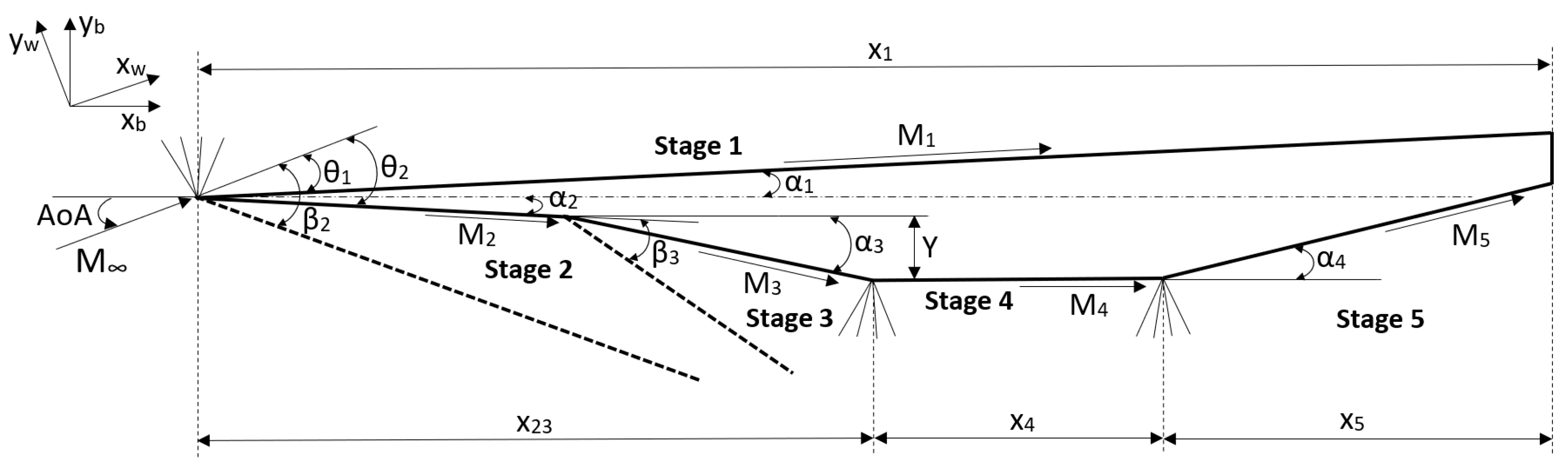
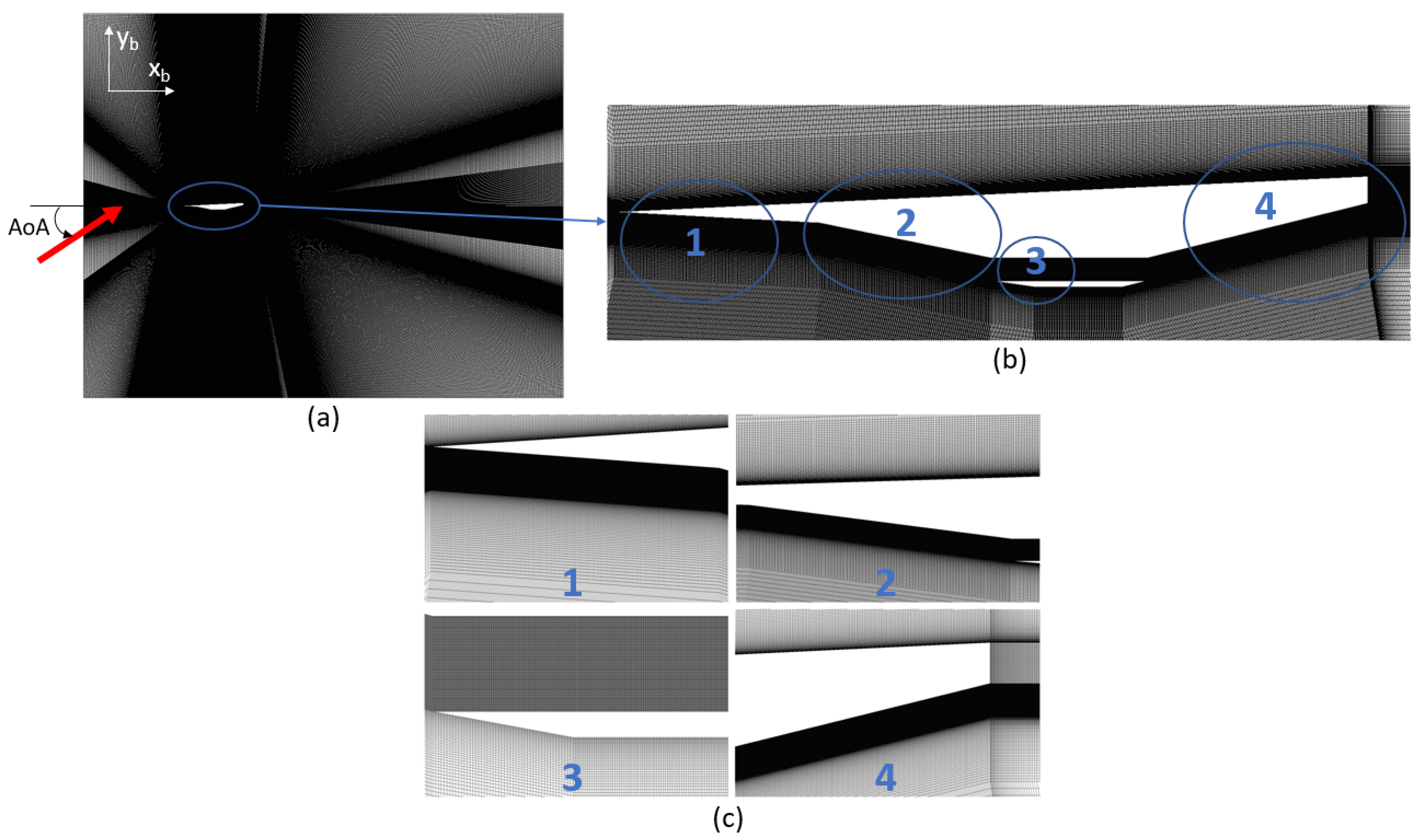
The comparison study between the analytical and CFD models was set to validate the CFD model used to develop the aerodynamic study. To do so, a CFD case with the aircraft geometry of Figure 1 was developed. Since the scramjet was neglected, few changes in the CFD domain were carried out: only the quadrilateral regions around the intrados of the aircraft were slightly modified, see Section 3. The structure of the mesh was maintained and its discretization was identical to that from Mesh 2 since it was the optimal one according to Section 4.1. All the other parameters such as the height of the cell in contact with the contours of the aircraft or the boundary conditions remained exactly the same. Furthermore, this case incorporated the same design angles as those from the analytical case and one single simulation per angle of attack was run, composing a total of 10 simulations.

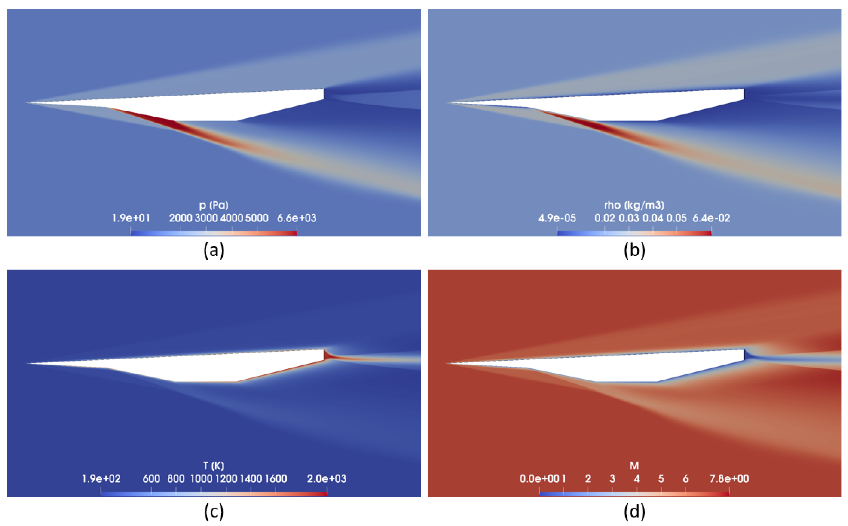
The pressure, density, temperature and Mach fields for $AoA=0^{\circ }$ of the CFD case with the scramjet neglected are depicted in Figure 3. The different discontinuities due to the oblique shock and Prandtl–Meyer expansion waves are clearly visible as well as the drastic expansion at the trailing edge. These physical phenomena are precisely explained in Section 4.5.

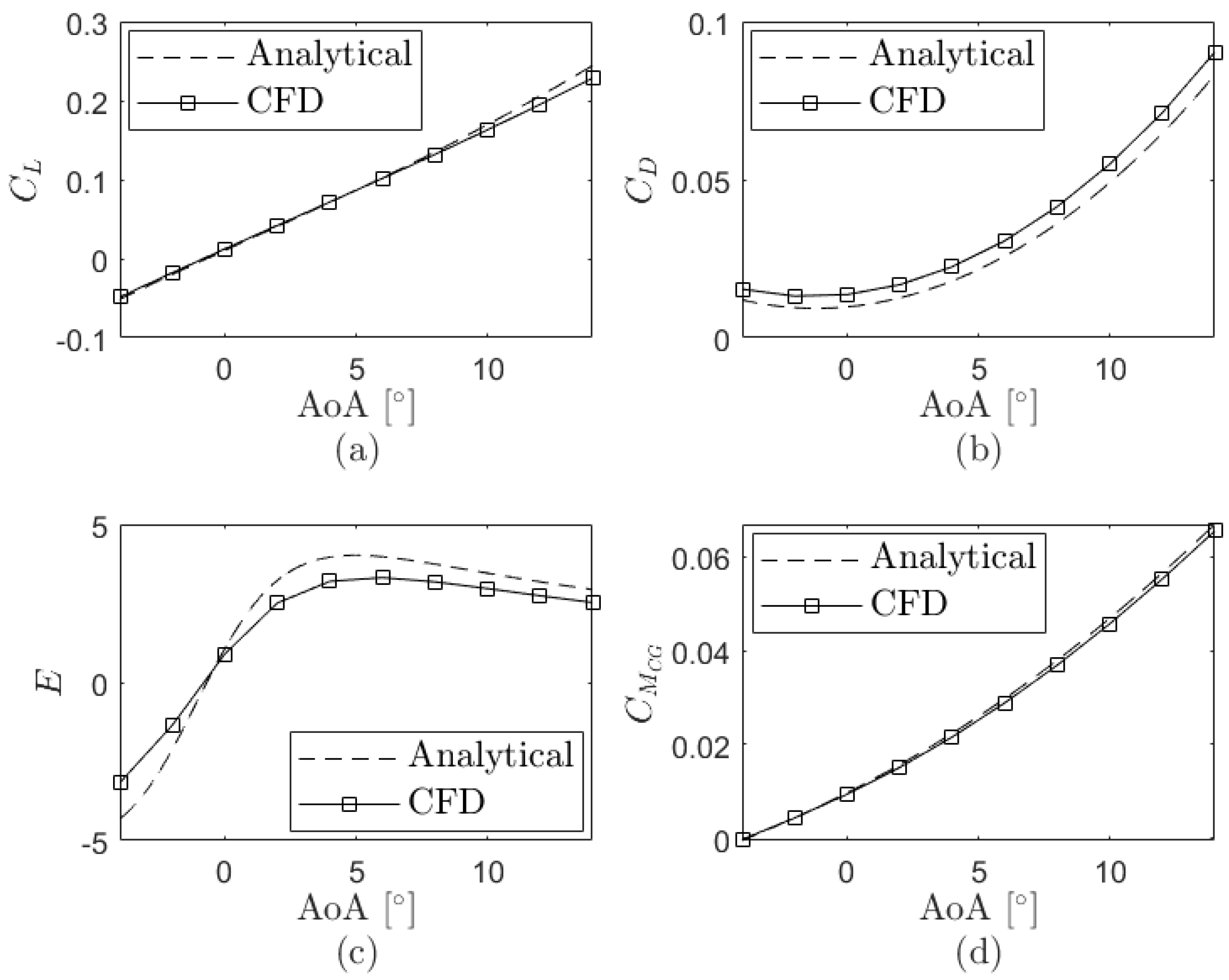
The comparison of the aerodynamic parameters is represented in Figure 4. Figure 4a shows that the CFD lift coefficient is lower than the analytical one in terms of absolute value; from $AoA=-4^{\circ }$ to $AoA=6^{\circ }$, the maximum deviation is under 1%, while from $AoA=8^{\circ }$ to $AoA={14}^{\circ }$, a maximum deviation of 5% is observed, approximately. The CFD drag coefficient is around 22% higher (Figure 4b). These differences are mainly caused by the viscous stresses considered in the CFD model since the analytical model did not include them. The aerodynamic efficiency is plotted in Figure 4c where, in terms of absolute value, the analytical aerodynamic efficiency is larger than the CFD for all the presented angles of attack since its drag coefficient is lower. In this case, the maximum efficiency in the analytical case is 18% higher than that of the CFD case (maximum deviation); such discrepancy is due to the viscous forces evaluated in the CFD simulations. Finally, according to Figure 4d, the pitching moment coefficient is similar in both types of studies and regardless of the angle of attack evaluated; only a maximum deviation of around 1% is observed.

Table 5. Aerodynamic parameters for the zero pitching moment ($C_{M_{CG}}=0$) and Vertical Force Balance (VFB) conditions of the CFD case with the scramjet neglected.

Condition	$\mathit{AoA}$ (${}^{\circ }$)	${\mathit{C}}_{\mathit{L}}$	${\mathit{C}}_{\mathit{D}}$	E	${\mathit{C}}_{{\mathit{M}}_{\mathit{CG}}}$
$C_{M_{CG}}=0$	−3.89	−0.0471	0.0152	−3.1	0
VFB	5.21	0.0899	0.0271	3.32	0.026

shows the analysis of the zero pitching moment and Vertical Force Balance conditions of the CFD case with the scramjet neglected. For the analytical case studied, the same analysis is presented in the following section,

Table 6. Aerodynamic parameters and shock wave angles for the zero pitching moment ($C_{M_{CG}}=0$) and Vertical Force Balance (VFB) conditions of the analytical case.

Condition	$\mathit{AoA}$ (${}^{\circ }$)	${\mathit{C}}_{\mathit{L}}$	${\mathit{C}}_{\mathit{D}}$	E	${\mathit{C}}_{{\mathit{M}}_{\mathit{CG}}}$	${\mathit{\beta }}_2$ (${}^{\circ }$)	${\mathit{\beta }}_3$ (${}^{\circ }$)	${\mathit{\beta }}_2^{\mathit{noc}}$ (${}^{\circ }$)	${\mathit{\beta }}_3^{\mathit{noc}}$ (${}^{\circ }$)
$C_{M_{CG}}=0$	−3.87	−0.0486	0.0116	−4.19	0	-	14.7	-	15.5
VFB	5.21	0.0899	0.0224	4.01	0.0268	14.7	16.9	15.5	15.5

. The characteristic angles of attack $Ao{A}_{(C_{M_{CG}}=0)}$ and $Ao{A}_{\left(VFB\right)}$ are almost the same as those calculated in the analytical study, compare Table 5 and Table 6. The CFD angle of attack that allows a zero pitching moment condition, $C_{M_{CG}}=0$, which is $-3.{89}^{\circ }$, is 0.5% higher than that of the analytical case, shown in Table 6. For the CFD angle of attack in which the aircraft flies with the Vertical Force Balance condition, which is $5.{21}^{\circ }$, it is exactly the same as the analytical one, shown in Table 6. As a result, for this last condition, the CFD lift coefficient is exactly the same as the analytical one and the CFD pitching moment coefficient $C_{M_{CG}}$ only differs by 3%. The CFD drag coefficient and CFD aerodynamic efficiency, however, differ by 21% and 17%, respectively, due to the consideration of the viscous effects in the CFD model.

This study shows that the analytical and CFD implementations generate very similar results. Only the drag coefficient and aerodynamic efficiency show some deviations, around 20% between both models.

In order to further validate the CFD model, the results of the CFD case 1 presented in Section 4.5 were compared by those presented in [2,3,8], where full three-dimensional CFD models and experimental tests at Mach number 6 were analysed. The parameters involved in the comparison study were the lift and drag coefficients for $AoA=2^{\circ }$, $AoA=4^{\circ }$, $AoA=8^{\circ }$ and $AoA={10}^{\circ }$. It is particularly remarkable to see that the experimental data presented in [2,8] is almost identical. In each of these two studies, there is also a good agreement between the experimental and CFD results. In addition to that, it is seen that the drag coefficients presented in the current paper are slightly smaller than those presented in the other studies. This fact is understandable since the wings, stabilizers and the lateral side of the aircraft are not considered in the present approach. It is also remarkable to see that the lift coefficients of the present paper are very close to the experimental and simulated ones obtained by [2,8]. For the drag coefficient, a maximum deviation of 37% between the experimental results from [2] and the results from the 2D CFD case 1 is obtained for an angle of attack of 2${}^{\circ }$. For the rest of the angles of attack evaluated, the $C_D$ average deviation is 17%. The maximum deviation for the lift coefficient is observed to be 20% for an angle of attack of 2${}^{\circ }$. The average $C_L$ deviation for the other angles of attack is 10%. Perhaps one positive conclusion extracted from the comparisons presented is that simple 2D simulations are capable of showing a trend in the same direction as full 3D experimental tests and CFD approaches. Furthermore, they show that the main body of the aircraft is responsible for most of the lift and drag exerted on the body.

4.4. Analytical Case and Geometric Modifications

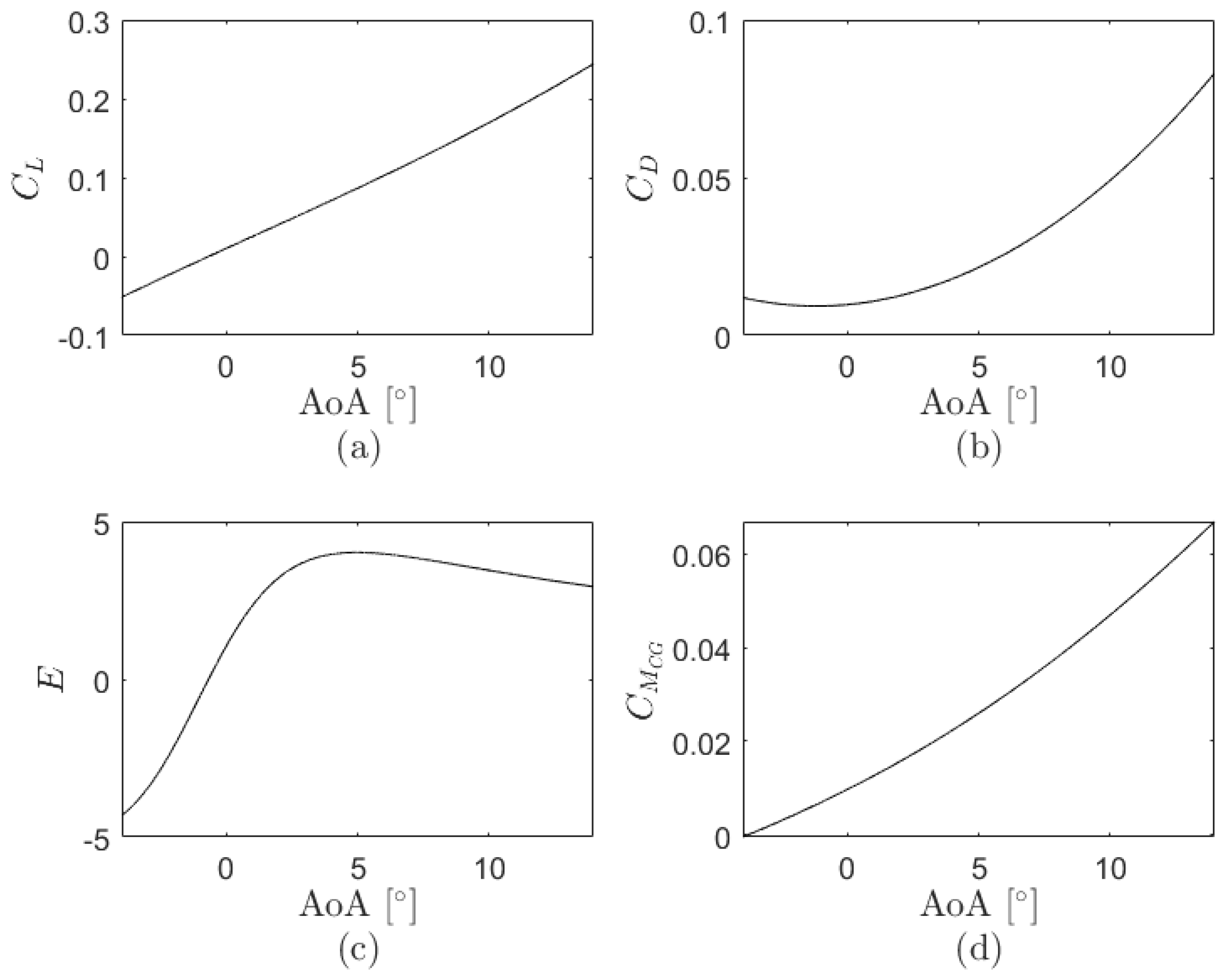
The dependence of the lift coefficient, drag coefficient, aerodynamic efficiency and pitching moment coefficient on the angle of attack of the analytical case studied at Mach 7 and an altitude of 30 km are depicted in Figure 5. In the analytical study, it was verified that the aerodynamic coefficients did not depend on the altitude, but the main parameters in which the aircraft flew with the Vertical Force Balance condition did. Within the angles of attack from −4${}^{\circ }$ to 14${}^{\circ }$, the lift coefficient increases almost linearly with the angle of attack (Figure 5a), while the drag coefficient does it in a parabolic way (Figure 5b). The stall in $C_L$ vs. $AoA$ is not contemplated since the effects of the boundary layer detachment were not considered. Efficiency E increases with the increase in the angle of attack, reaches its maximum value of 4.02 at $AoA=4.{94}^{\circ }$, and then decreases (Figure 5c). Finally, the pitching moment coefficient, which was considered to be positive in the pitch up of the aircraft, also increases approximately in a linear way with the $AoA$ (Figure 5d). As its gradient, known as the longitudinal static stability index, is positive, the aircraft is unstable with regard to any disturbance in the angle of attack; when $\Delta AoA>0$, then $\Delta C_{M_{CG}}>0$ and the aircraft tends to raise its nose.

Table 6 shows these coefficients in addition to the shock wave angles ${\beta }_2$ and ${\beta }_3$ for the zero pitching moment and Vertical Force Balance conditions as well as the corresponding $Ao{A}_{(C_{M_{CG}}=0)}$ and $Ao{A}_{\left(VFB\right)}$. Both parameters ${\beta }_2^{noc}$ and ${\beta }_3^{noc}$ are the shock wave angles of stages 2 and 3, respectively, in which the aircraft would fly with the nose optimised configuration according to the defined angles of attack. This configuration can be considered if the deviations between them and ${\beta }_2$ and ${\beta }_3$ are under 10%. The zero pitching moment condition is achieved for $Ao{A}_{(C_{M_{CG}}=0)}<0$, which leads to a negative lift coefficient and aerodynamic efficiency, and a Prandtl–Meyer expansion wave is originated at the beginning of stage 2. Moreover, since ${\beta }_3$ is very close to ${\beta }_3^{noc}$, the aircraft can be considered to fly with the nose optimised configuration. In case of the Vertical Force Balance condition, since $Ao{A}_{\left(VFB\right)}=5.{21}^{\circ }$, the lift coefficient is positive and the aerodynamic efficiency is almost maximum, but $C_{M_{CG}}>0$. As ${\beta }_2$ differs by 5% from ${\beta }_2^{noc}$ and ${\beta }_3$ by 8% from ${\beta }_3^{noc}$, the aircraft can also be considered to fly with the shock waves of stages 2 and 3 focusing on the tip of the lower edge of the scramjet.

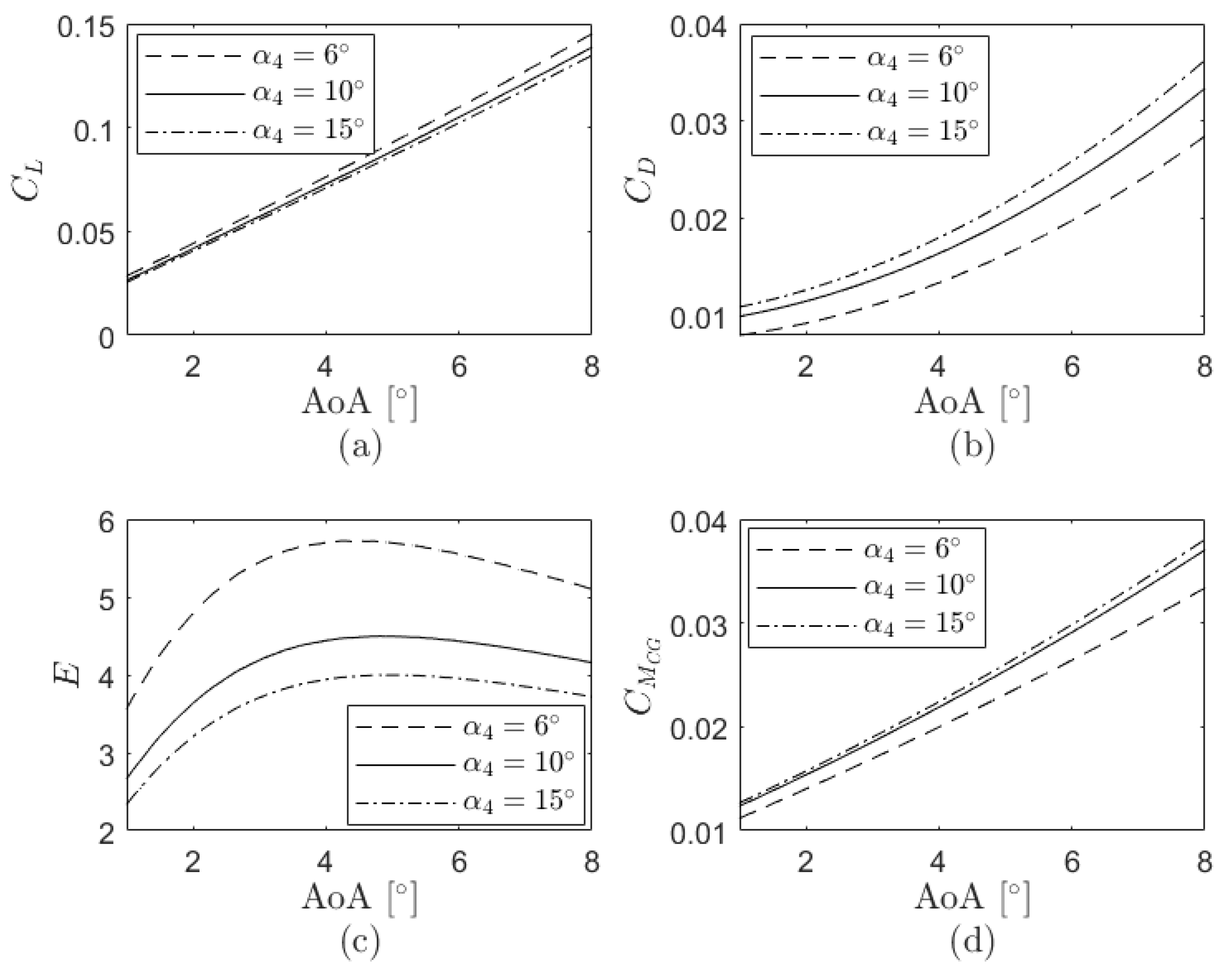
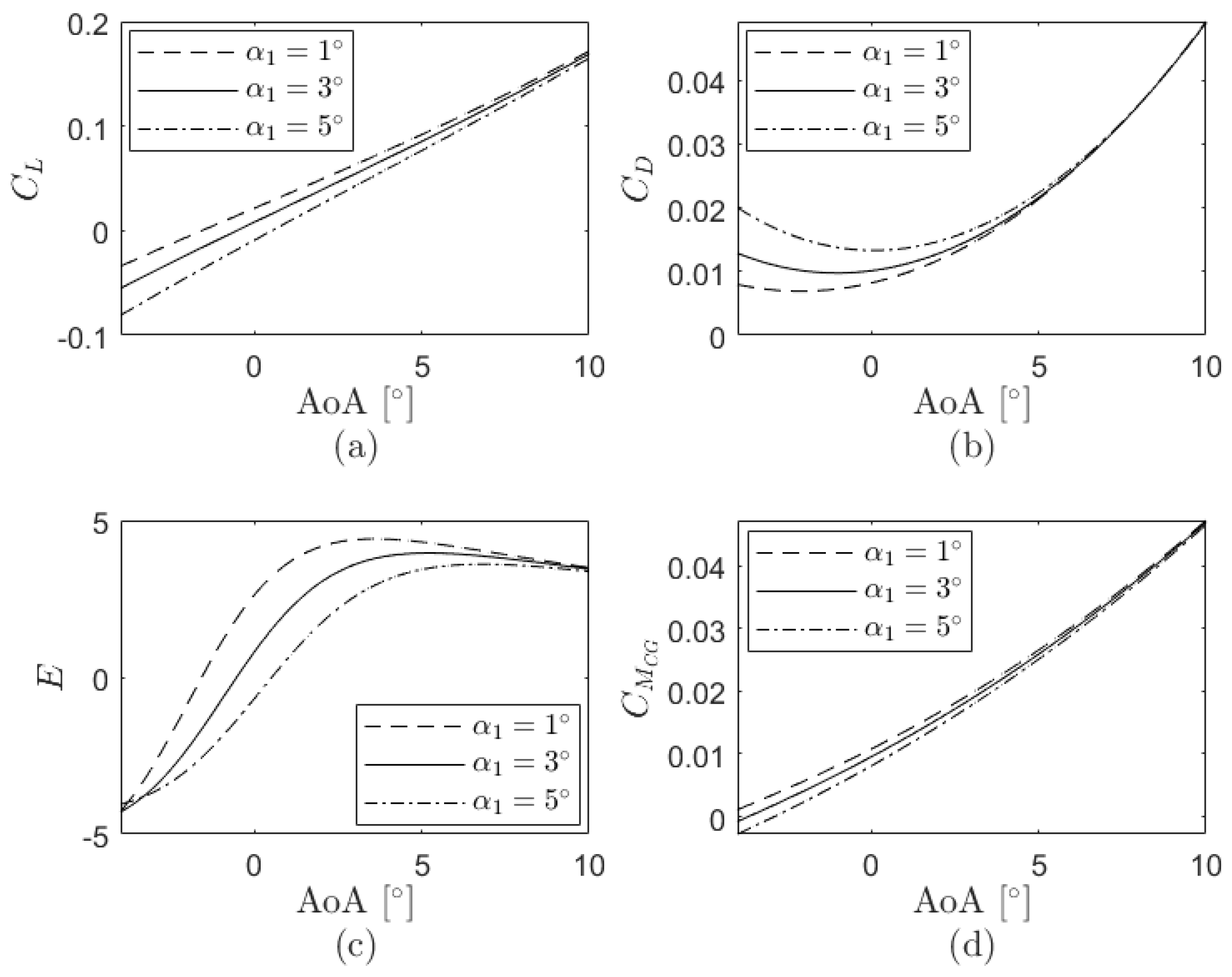
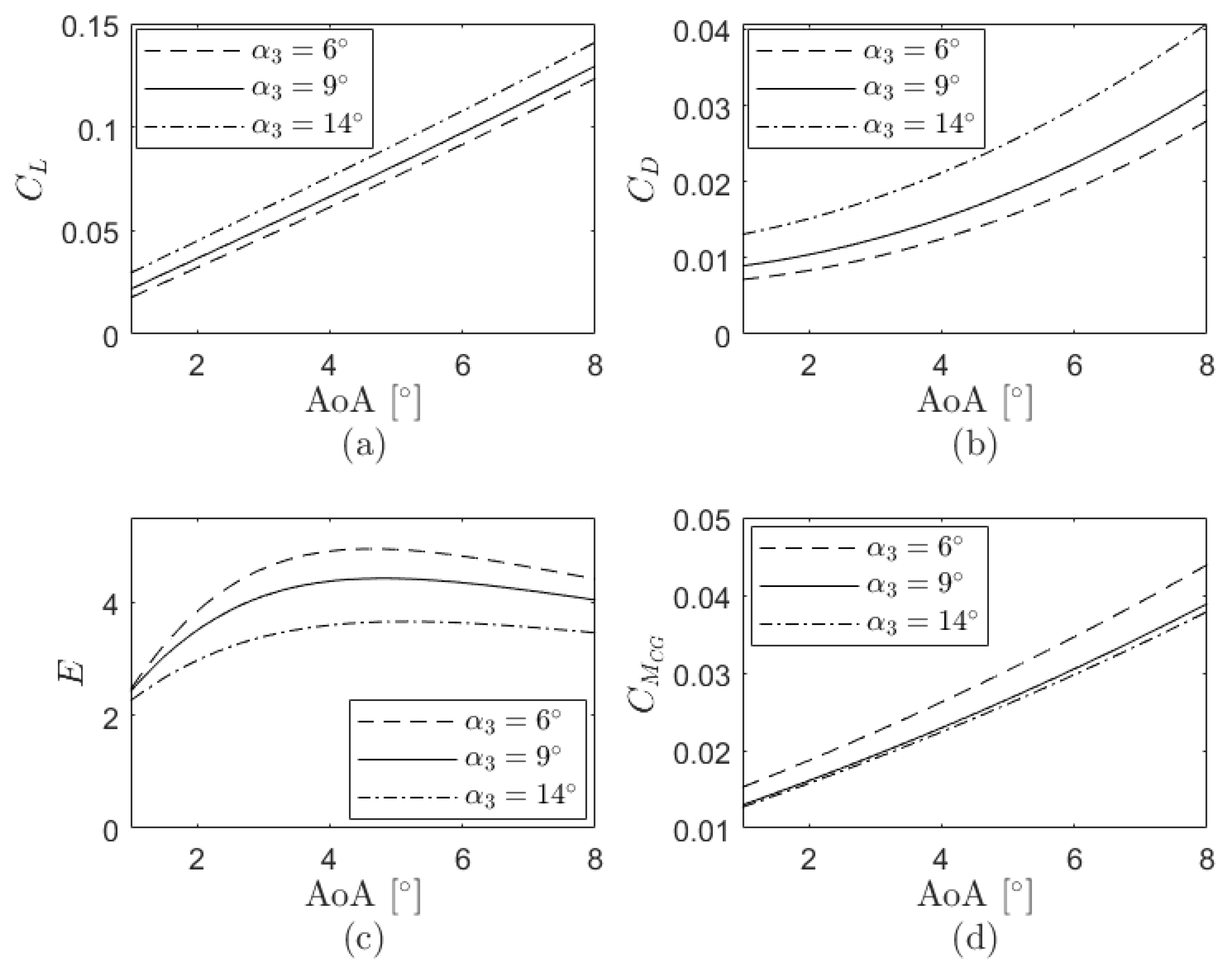
The variations of the lift coefficient, drag coefficient, aerodynamic efficiency and pitching moment coefficient as a consequence of the changes in the design angles are evaluated next. These parameters in terms of the angle of attack for different ${\alpha }_1$ and maintaining constant the remaining design angles (${\alpha }_2$, ${\alpha }_3$ and ${\alpha }_4$) as those from the analytical case are presented in Figure 6, where a reduction of ${\alpha }_1$ brings an increase of the lift coefficient, aerodynamic efficiency and pitching moment coefficient and a decrease of the drag coefficient. 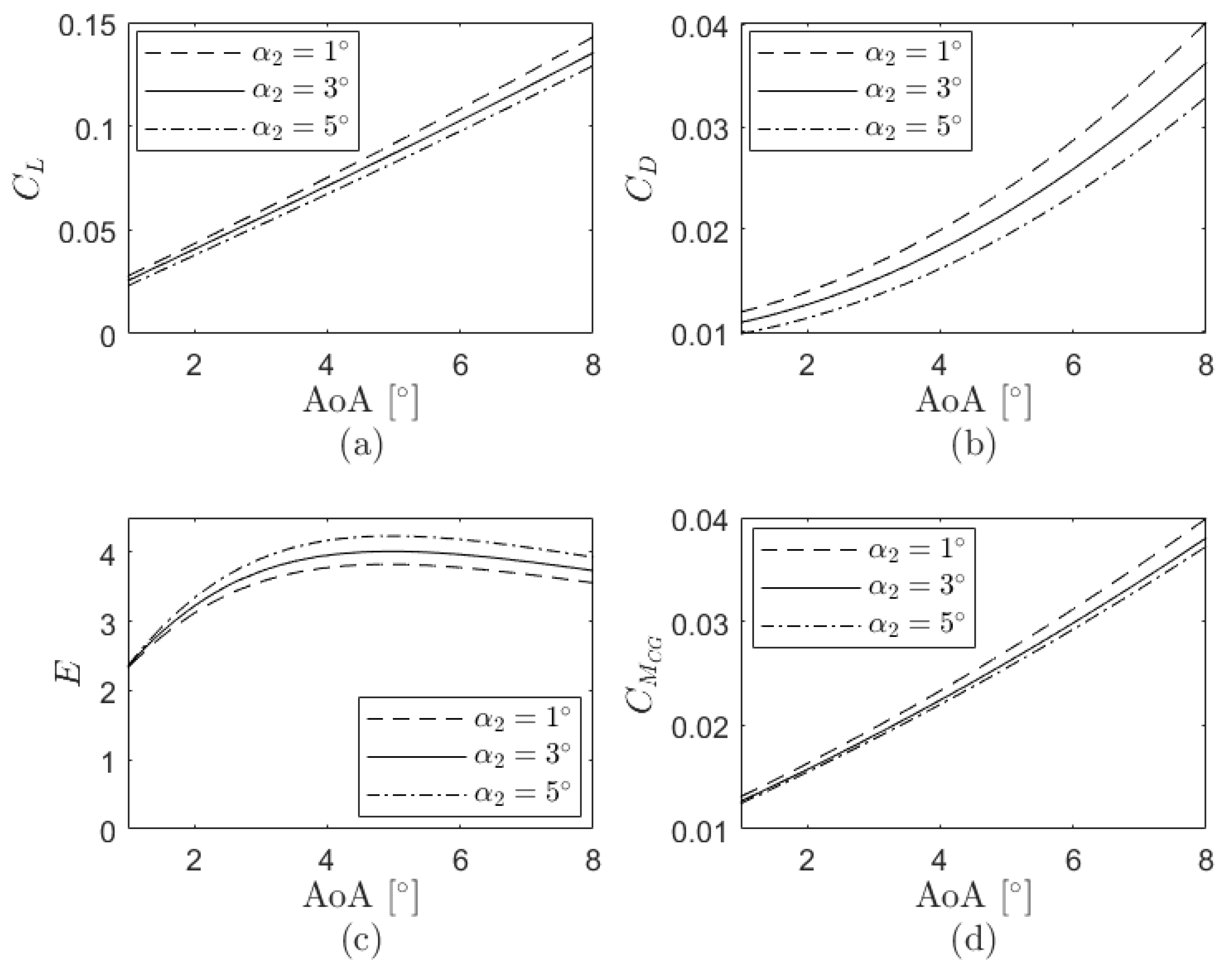As seen in Figure 7, decreasing ${\alpha }_2$ increases the lift, drag and pitching moment coefficients while the aerodynamic efficiency decreases. According to Figure 8, a reduction of ${\alpha }_3$ implies an increase of the pitching moment coefficient and aerodynamic efficiency and a decrease of the lift and drag coefficients. Figure 9 finally shows the modifications of the aerodynamic coefficients due to the changes in ${\alpha }_4$ where, in this particular case, a decrease of this design angle comes with an increase of the lift coefficient and aerodynamic efficiency and a decrease of the drag and pitching moment coefficients. Overall, since the surface of stage 1 is far bigger than that of the other stages, the variations of the aerodynamic parameters are more significant when ${\alpha }_1$ is manipulated than when the other design angles are modified. Although modifications on ${\alpha }_1$ are smaller than those on the other angles, the differences of the aerodynamic coefficients are more notorious in the first case.

4.5. CFD Cases

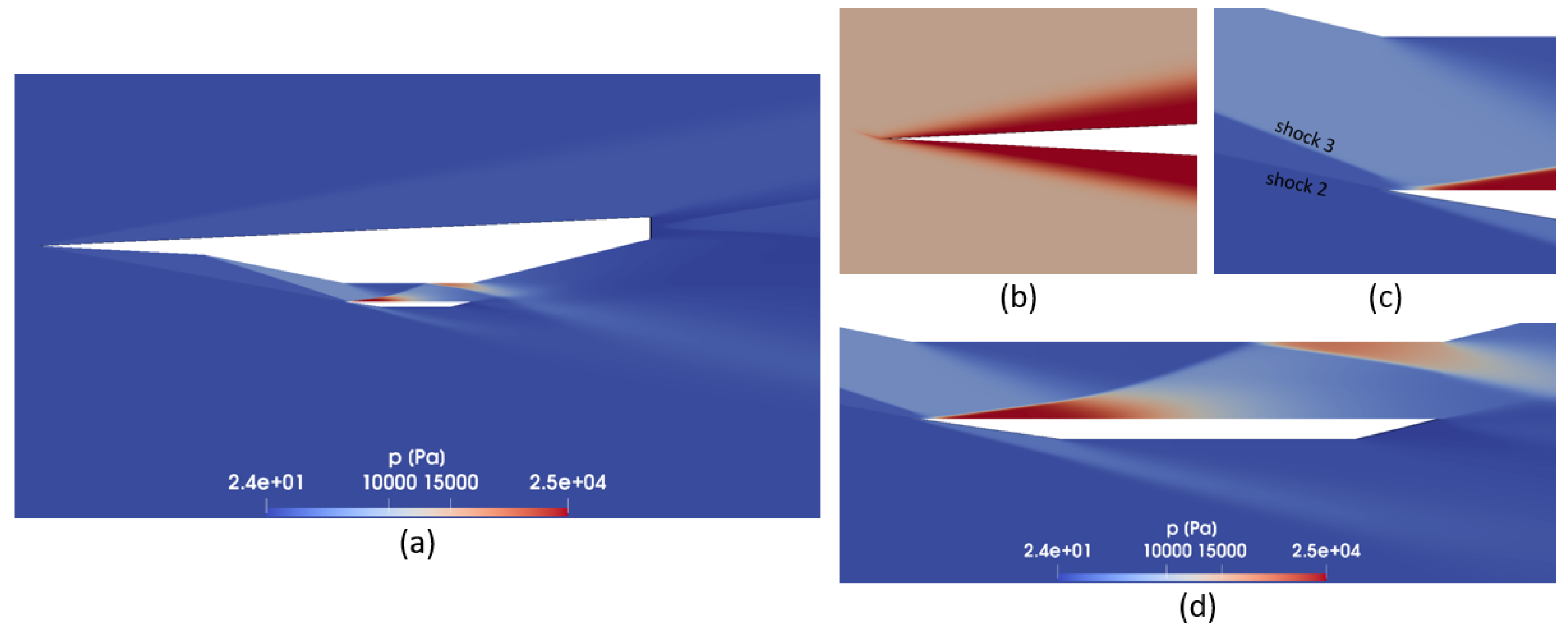
Case 1 is initially presented with the variation of the pressure field throughout the aircraft at a zero angle of attack in Figure 10a. Since $AoA<{\alpha }_1$, a shock wave is produced at the beginning of the extrados where, consequently, the pressure is increased and remains approximately constant along the surface. This phenomenon is also present in the aircraft nose (stages 2 and 3); in case of stage 3, the increase of pressure is more significant due to the difference in the design angles (${\alpha }_3>>{\alpha }_1\&{\alpha }_2$, see Table 3).

Figure 10b shows that shock waves of stages 1 and 2 are completely attached to the sharp leading edge of the wedge. This fact is given because of the high Mach number where X-43A flies and the small wedge angle that presents at the leading edge. X-43A uses the fuselage nose part to form the shock in front of the intake. Theoretically (according to the analytical model), the aircraft should fly with the nose optimised configuration under those conditions of design angles and $AoA$. 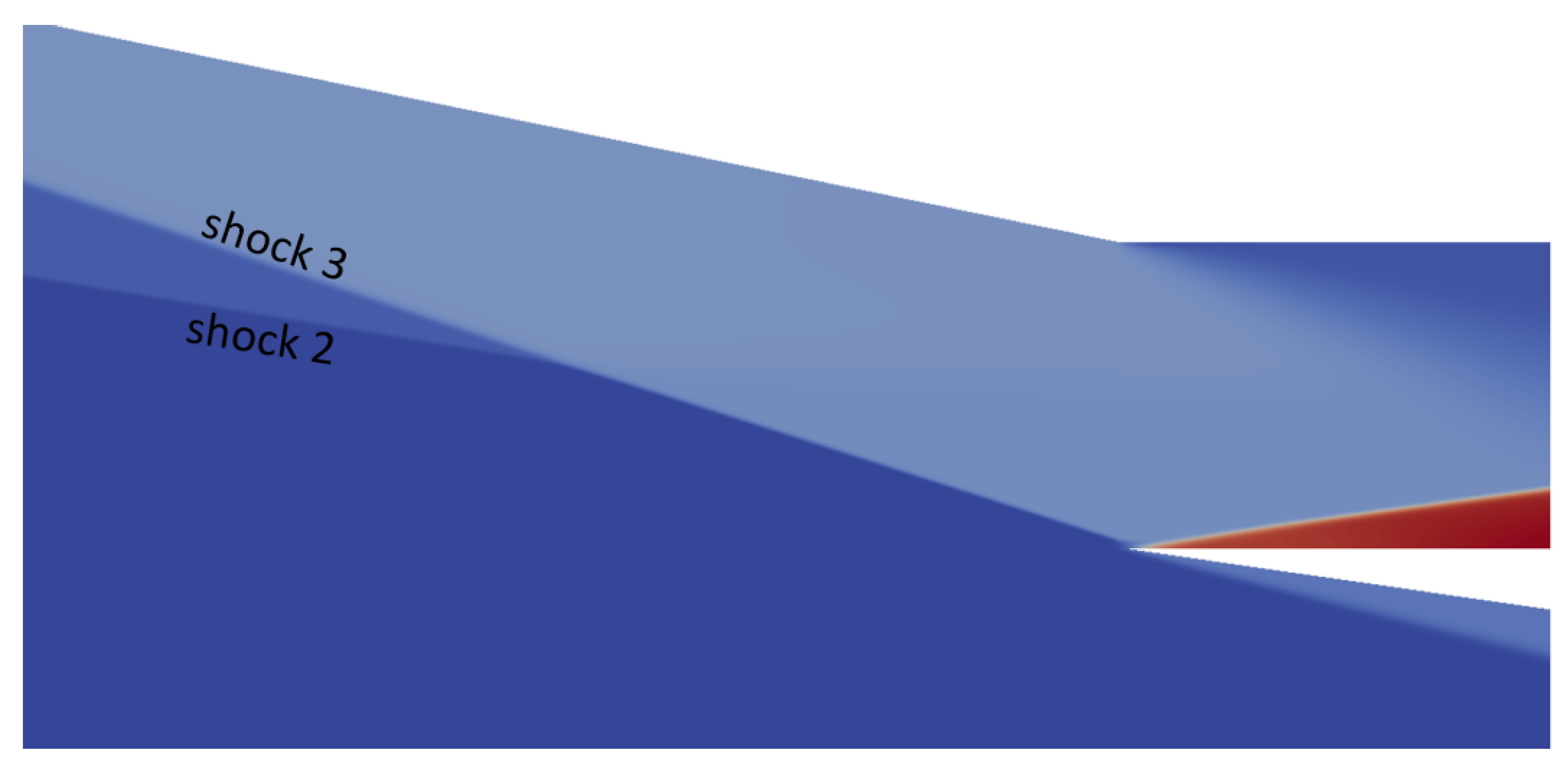Notice that in this case a different colour scale has been used to represent this phenomenon. Focusing on Figure 10c, shock 2 (which is the one formed at the beginning of stage 2) is focused on the tip of the lower edge, while shock 3 (the one that corresponds to the shock wave created at the beginning of stage 3) is slightly deflected into the entrance of the throat.

Inside the scramjet, different things occur together (see Figure 10d for more detail). On the one hand, the flow expands as a Prandtl–Meyer expansion wave being produced at the end of stage 3. As a result, there is a small region situated in the upper left side in which the pressure decreases from that of the previous stage. On the other hand, shock 3 reflects from the lower edge generating a new shock, which, in turn, reflects from the upper edge forming, once again, another shock wave. In other words, two regular reflections in steady flow inside the engine are created. The first reflection leads to a high pressure region downstream at about 25 kPa, while the pressure after the second reflection is 15 kPa approximately. These differences are caused by the incident pressure of each reflection shock (the one of the first reflection shock is bigger than that of the second reflection shock) which, overall, translates into an energy dissipation of these reflection shock waves along the scramjet. In addition to that, after the first reflection, the flow is theoretically parallel to both wedges. This phenomenon is known as the shock diamond and provides some regions with strong adverse pressure gradients which induce flow separation. Finally, at the end of the upper right side of the scramjet, a Prandtl–Meyer expansion wave is originated. The pressure decreases and remains constant along the surface all the way to the trailing edge; there, the expansion process is so drastically that the pressure goes down to 20 Pa approximately, which enables the creation of some vortex.

Overall, all the waves originating along the aircraft are dissipated slowly downstream until the outlet boundary section.

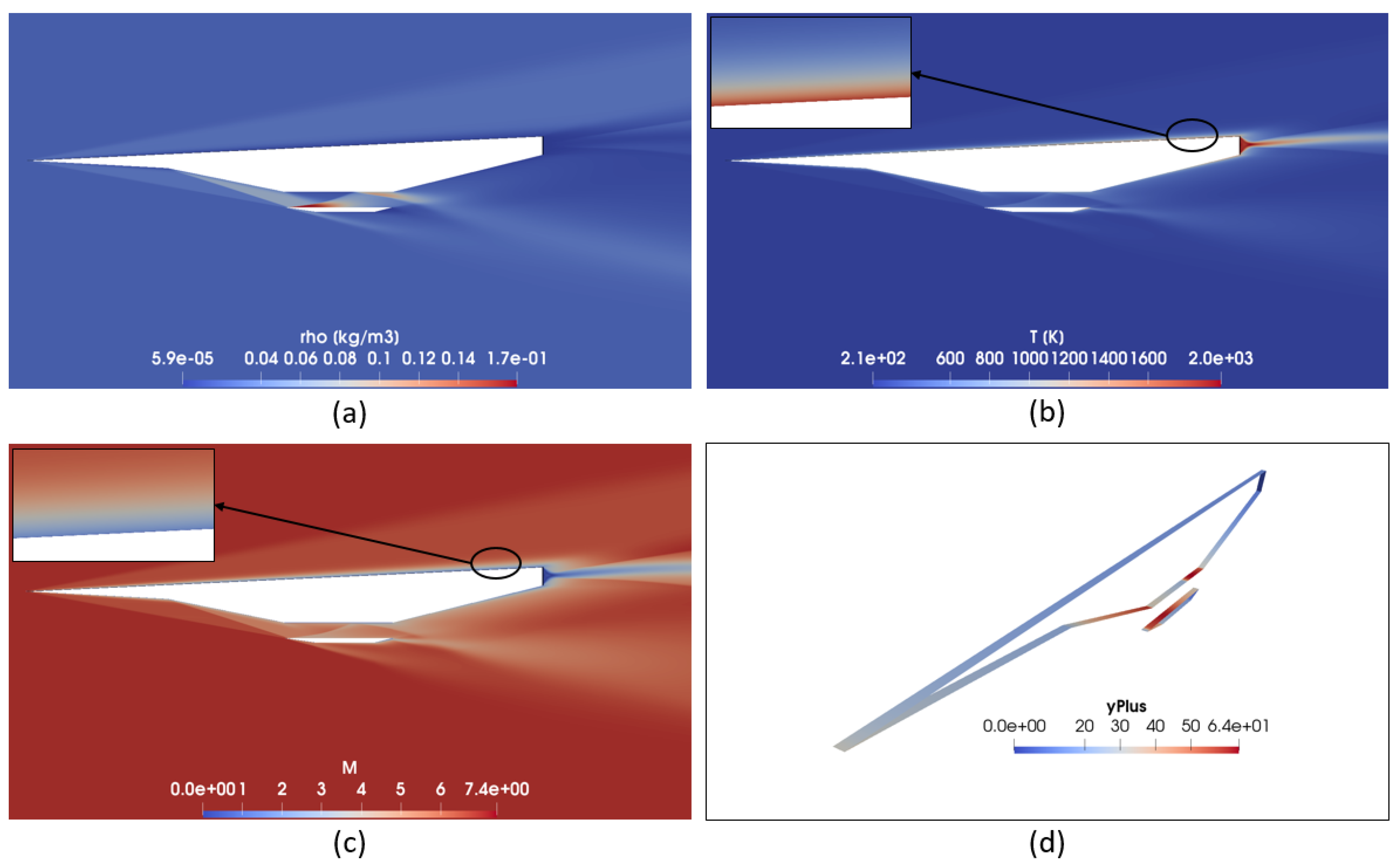
The density, temperature and Mach fields of the domain for the same angle of attack are depicted in Figure 11 in addition to the $y^{+}$ distribution along the walls of the aircraft. The density behaviour (Figure 11a) is almost the same as the pressures: a high density in some regions inside the scramjet and an almost zero one along the trailing edge. In addition, as the flight altitude is high, the density values are relatively small as well as those from pressure. Since the air was considered to be a perfect gas, the density along the surfaces is reduced due to the high temperatures there. In case of the temperature field (Figure 11b), two remarkable things are given in addition to the discontinuities caused by the oblique shock and Prandtl–Meyer expansion waves. Firstly, some aircraft contours are illuminated or, equivalently, the temperature is higher. This means that these regions capture the thermal boundary layer; the surface temperature is higher and decreases with the normal direction until arriving to the freestream temperature, which it keeps constant. From a theoretical point of view, this high temperature is caused by the viscous stresses, which, in turn, are caused by the enormous velocity gradients along the boundary layer. According to Figure 11d, these regions are the same as those with low $y^{+}$ values, which, evidently, translates into a more precise capture of the boundary layer. Contrary to that, other regions where the pressure is relatively high (e.g., some parts of the walls inside the scramjet or the wall of stage 3), the maximum $y^{+}$ values are around 50 or, in other words, are relatively high and, consequently, the temperature gradients can not be properly visualised. In fact, the $y^{+}$ of the different surfaces of the aircraft are extremely different due to the drastic changes of the air properties that are caused by the shock and Prandtl–Meyer expansion waves phenomena. Secondly, the temperature around the trailing edge is extremely high and decreases gradually downstream producing two lines around it. These lines represent discontinuities such as expansion waves, forming a triangle that dissipates with the distance. Finally, for the Mach field (Figure 11c), a zero Mach number is found in some aircraft contours, which translates into a zero flow velocity. In fact, these regions are also the same as those with low $y^{+}$, meaning that some part of the boundary layer is captured. The Mach number starts being zero on the surface and increases gradually along its normal direction until arriving to the Mach number downstream the wave. Overall, the Mach field has the same behaviour as the pressure and temperature fields. The oblique and Prandtl–Meyer expansion waves are clearly delimited, and the regions where the pressure increases, the Mach number decreases and vice versa. As well as in the temperature field, a large fluid expansion occurs at the trailing edge; the Mach number falls to zero and increases progressively downstream.

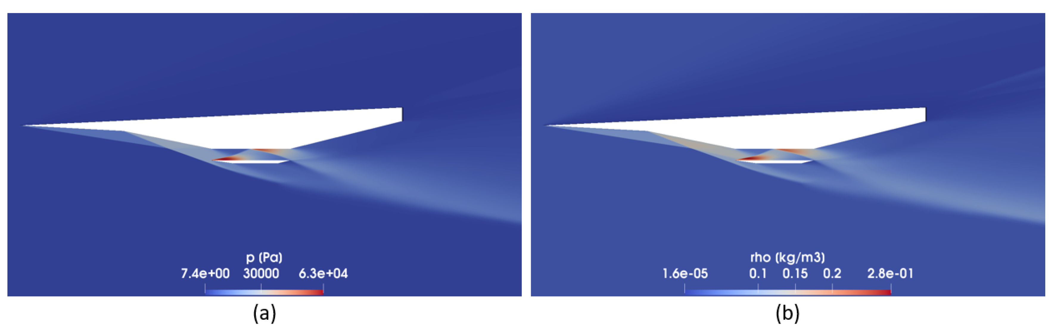
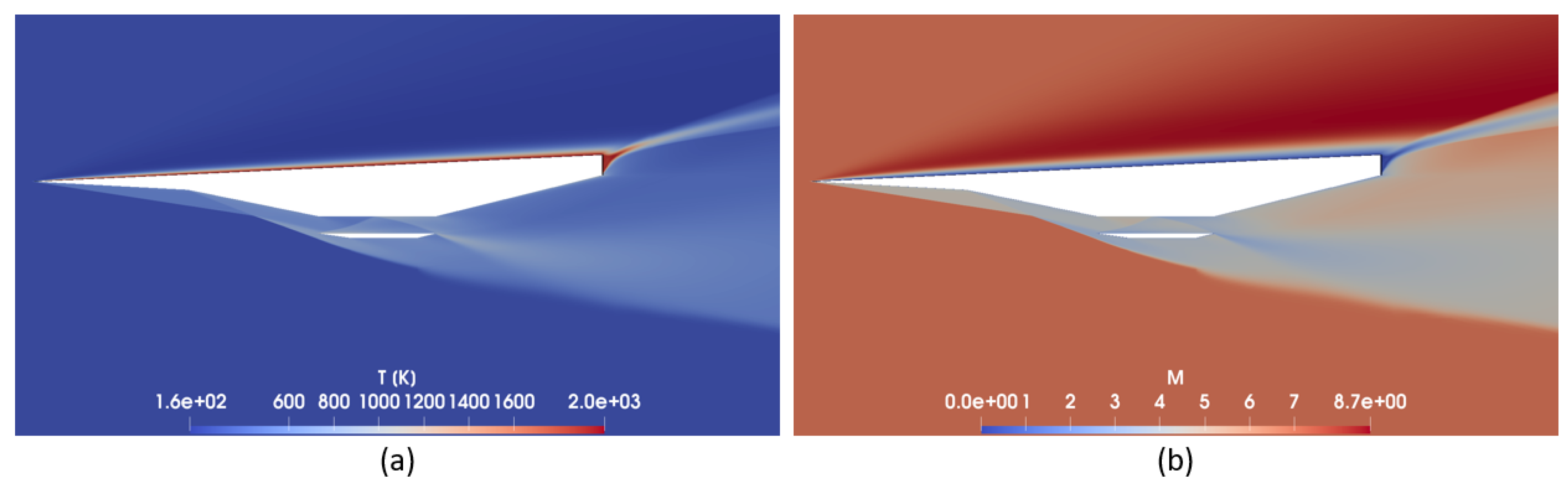
The main fields for $AoA={14}^{\circ }$ of case 1 are also evaluated, see Figure 12 and Figure 13. Under these conditions, a Prandtl–Meyer expansion wave is originated at the beginning of extrados, thus the pressure (Figure 12a), density (Figure 12b) and temperature (Figure 13a) decrease and the Mach number (Figure 13b) increases. The increase of the angle of attack causes a displacement to the left side of shock 3, which cuts the one coming from stage 2 due to its superiority in pressure strength and incapacitates it to reach the scramjet. A third reflection takes place at the end of the tip of the scramjet, which is almost imperceptible due to its weakness. Finally, the increase of the $AoA$ also produces an increase of the pressure gradients inside the scramjet in addition to a higher curvature of shock 3 and the waves created at the trailing edge.

For $AoA=4^{\circ }$ (Figure 14), the aircraft can be considered to fly with the nose optimised configuration since the oblique shock wave formed at the beginning of stage 3 is focused on the tip of the lower edge of the scramjet.

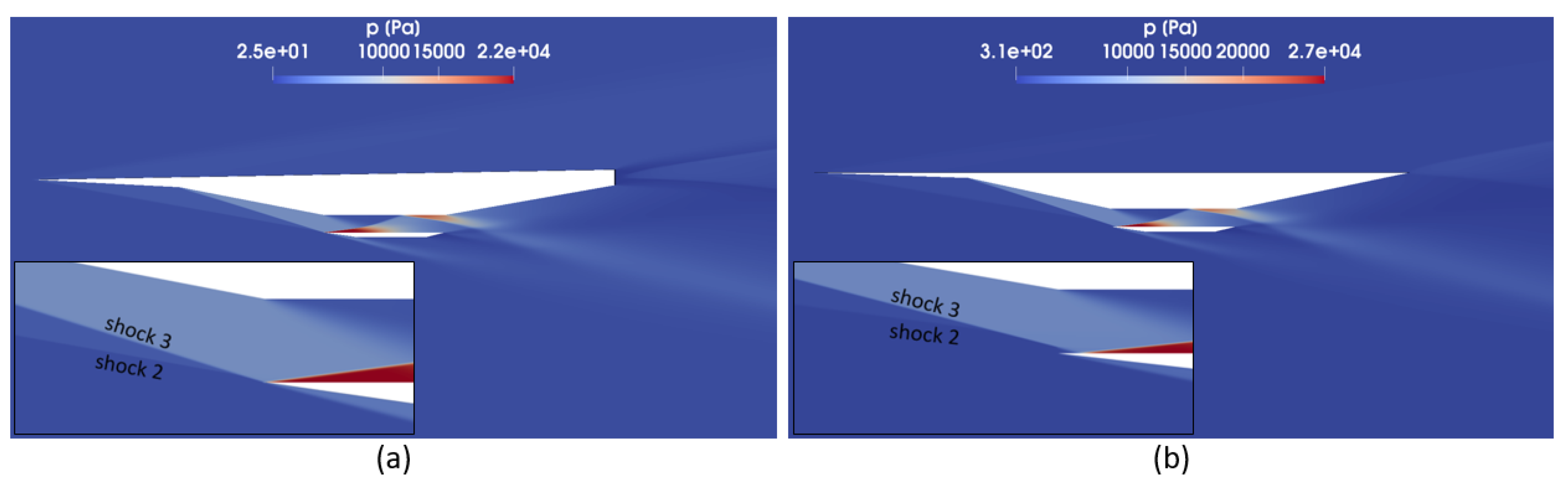
The pressure field of the other two CFD cases studied, case 2 and case 3 defined in Table 3 for $AoA=0^{\circ }$, is presented in Figure 15. Case 2 was designed to fly with the nose optimised configuration for $AoA=0^{\circ }$ as seen in Figure 15a. In addition to that, the design angles ${\alpha }_1$ and ${\alpha }_4$ were slightly reduced from case 1 in order to have a better aerodynamic performance according to the results obtained of the analytical model, see Figure 6 and Figure 9; the maximum reached pressure (situated in the lower edge of the scramjet) is about 22 kPa instead of the 25 kPa observed in case 1 which, in the end, translates into a higher lift. Case 3 was not only created to improve the aerodynamics of the aircraft by reducing ${\alpha }_1$ and ${\alpha }_4$ from case 1, but also to avoid the drastic expansion and, consequently, an extremely low pressure and velocity and a high temperature at the trailing edge by eliminating its surface. In this case, for $AoA=0^{\circ }$, shock 3 is slightly deflected into the entrance of the throat as seen in Figure 15b. Furthermore, it was seen that the aircraft flew with the nose optimised configuration for $AoA=4^{\circ }$ (this corresponding simulation is not presented in the study). The maximum pressure is focused along the scramjet and is about 27 kPa. Furthermore, as the surface of the trailing edge is eliminated, the drastic expansion is not observed as in the other cases.

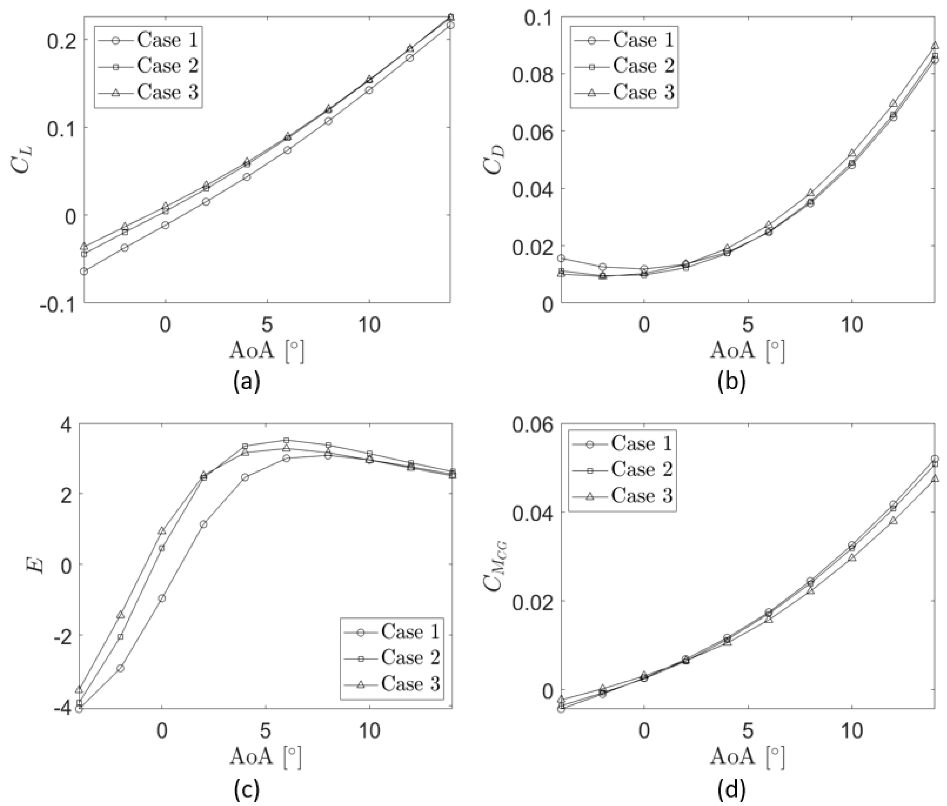
The integral aerodynamic characteristics $C_L$, $C_D$, E and $C_{M_{CG}}$ in terms of the angle of attack for the three CFD cases are shown in Figure 16. As seen in Figure 16a, case 3 has the highest lift coefficient until $AoA=6^{\circ }$, where it is approximately the same as that of case 2. Case 1, however, has the lowest lift coefficient with a negative lift coefficient for $AoA=0^{\circ }$. According to Figure 16b, case 1 has the highest drag coefficient up to $AoA=2^{\circ }$, where the first place is replaced by case 3, and case 1 has a very similar drag coefficient as case 2. The combination between the lift and drag coefficients leads to the aerodynamic efficiency in terms of the $AoA$ (Figure 16c). Both cases 2 and 3 have a similar E; the aerodynamic efficiency of case 3 is higher for $AoA={\left[-4,-2,0,2\right]}^{\circ }$ and lower for the other angles of attack. Therefore, according to this graph, the maximum aerodynamic efficiency of case 2 is the highest one ($E_{max}=3.52$ for $AoA=6^{\circ }$), followed by the one in case 3 ($E_{max}=3.28$ for $AoA=6{}^{\circ }$) and finally case 1 ($E_{max}=3.09$ for $AoA=8^{\circ }$). In addition, from $AoA={10}^{\circ }$, all cases seem to converge to a certain value. Finally, the behaviour of the pitching moment coefficient through the different angles indicates a longitudinal instability condition with regard to any perturbation of the $AoA$ (Figure 16d); cases 1 and 2 are mostly similar according to this graph, while case 3 has the highest pitching moment coefficient for $AoA={\left[-4,-2,0\right]}^{\circ }$ and the lowest one for the other angles of attack. Therefore, as stated before, cases 2 and 3, which are very similar from an aerodynamic point of view, offer, in general, a better aerodynamic performance than the one from case 1.

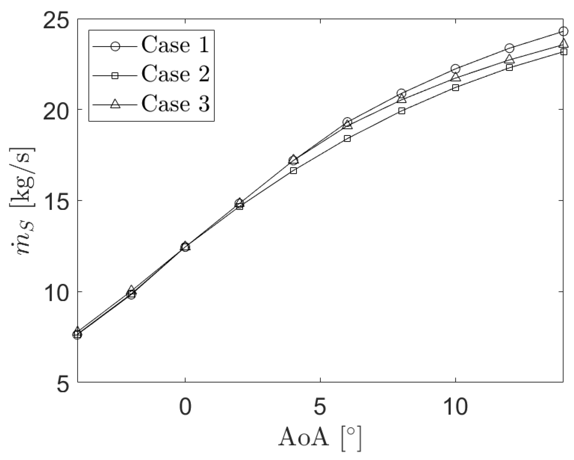
The mass flow rate throughout the scramjet in terms of the angle of attack of the three CFD cases is presented in Figure 17 where, for the three cases, increases with it. In addition to that, all cases have approximately the same mass flow rate for $AoA={\left[-4,-2,0\right]}^{\circ }$; at higher angle of attack, the mass flow rate of case 1 is the highest one, followed by the one from case 2 and finally case 3. For $AoA=4^{\circ }$, the mass flow rate of cases 1 and 3 are higher than that of case 2 as the aircraft flies with the nose optimised configuration.

All of the presented parameters of the three CFD cases are shown in

Table 7. Aerodynamic parameters and mass flow rate for the zero pitching moment condition ($C_{M_{CG}}=0$) of the three CFD cases.

Case	${\mathit{AoA}}_{({\mathit{C}}_{{\mathit{M}}_{\mathit{CG}}}=0)}$ (${}^{\circ }$)	${\mathit{C}}_{\mathit{L}}$	${\mathit{C}}_{\mathit{D}}$	E	${\mathit{C}}_{{\mathit{M}}_{\mathit{CG}}}$	${\dot{\mathit{m}}}_{\mathit{S}}$ (kg/s)
1	−1.45	−0.0299	0.0122	−2.45	0	10.55
2	−1.53	−0.0139	0.0094	−1.48	0	10.49
3	−2.15	−0.0149	0.0093	−1.6	0	9.87

and

Table 8. Aerodynamic parameters and mass flow rate for the Vertical Force Balance condition (VFB) of the three CFD cases.

Case	${\mathit{AoA}}_{\left(\mathbf{VFB}\right)}$ (${}^{\circ }$)	${\mathit{C}}_{\mathit{L}}$	${\mathit{C}}_{\mathit{D}}$	E	${\mathit{C}}_{{\mathit{M}}_{\mathit{CG}}}$	${\dot{\mathit{m}}}_{\mathit{S}}$ (kg/s)
1	6.96	0.0899	0.0291	3.09	0.0207	20.09
2	6.14	0.0899	0.0255	3.52	0.0176	18.5
3	6.03	0.0899	0.0274	3.28	0.0158	19.12

for the zero pitching moment and Vertical Force Balance conditions, respectively. For the first condition, all cases have a negative lift coefficient and aerodynamic efficiency since the angle of attack is negative; case 2 presents a lift coefficient slightly least negative than the rest, while case 3 has the lowest drag coefficient. This leads case 2 to reach the least negative aerodynamic efficiency and case 3 to have the lowest $Ao{A}_{(C_{M_{CG}}=0)}$. It is important to highlight that the negative lift coefficient obtained in the present study is caused by the non consideration of the stabilizers. These elements would be able to compensate this coefficient allowing the aircraft to fly. For the second condition, case 2 also gets the highest aerodynamic efficiency and the lowest drag coefficient. However, case 3 achieves this condition with a lower $Ao{A}_{\left(VFB\right)}$, which translates into a better aerodynamic performance from a “lift point of view”. In addition to that, when the Vertical Force Balance condition is achieved, all cases present their corresponding maximum aerodynamic efficiency. Despite case 1 being the worst case in all aerodynamic aspects, it has the highest mass flow rate for both conditions.

5. Conclusions

A 2D aerodynamic study of the NASA’s X-43A hypersonic aircraft has been performed using two approaches. The first one (analytical) neglects the effects of the scramjet and is based on the resolution of the oblique shock wave and Prandtl–Meyer expansion wave theories, while the second one (computational) considers the real shape of the aircraft and involves the use of a CFD package. On the one hand, in the analytical model, only one single case whose design angles allowed the aircraft to fly with the nose optimised configuration for $AoA=0^{\circ }$ has been strictly studied for $M_{\infty }=7$ and $z=30$ km. The lift coefficient, drag coefficient, aerodynamic efficiency and pitching moment coefficient in terms of the angle of attack with $AoA\in {\left[-4,14\right]}^{\circ }$ have been depicted. The linearity of the lift coefficient, the second order polynomial dependence of the drag coefficient, the increase and decrease of the aerodynamic efficiency with $E_{max}=4.02$ for $AoA=4.{94}^{\circ }$ and the longitudinal instability of the aircraft have been observed. Afterwards, the study of the pitching moment and Vertical Force Balance conditions have been defined. For the zero pitching moment condition, the lift coefficient has resulted in being negative and, consequently, a negative aerodynamic efficiency has been obtained. Contrary to that, for the Vertical Force Balance condition, the aircraft has reached its maximum aerodynamic efficiency. In both conditions, the aircraft has been analysed to be flying with the nose optimised configuration. The discussion of the analytical model has been closed by the changes of the aerodynamic parameters (lift and drag coefficients, aerodynamic efficiency and pitching moment coefficient) with the design angles. The changes of these parameters have been far more significant with the manipulation of ${\alpha }_1$. Furthermore, it has been observed that the aerodynamic efficiency of the aircraft increased with the decrease in the design angles ${\alpha }_1$ and ${\alpha }_4$.

On the other hand, in the CFD model, three different cases with different design angles have been analysed for $M_{\infty }=7$, $z=30$ km and $AoA={\left[-4,-2,0,2,4,6,8,10,12,14\right]}^{\circ }$. The pressure, density, temperature and Mach fields of case 1 have been shown for $AoA=0^{\circ }$ and $AoA={14}^{\circ }$ as well as the pressure field for the other cases at a zero angle of attack. Firstly, the oblique shock and Prandtl–Meyer expansion waves along the physical domain have been visualised as well as an attachment condition at the leading edge for all situations. Case 1 has appeared to be flying with the nose optimised configuration for $AoA=4^{\circ }$ (different from the $0^{\circ }$ of the analytical study) as well as case 3, while for case 2 it has been imposed to be for $AoA=0^{\circ }$. Secondly, the shock diamond inside the scramjet with two reflection waves causing high pressure gradients has been confirmed. Thirdly, an expected flow disturbance caused by the drastic flow expansion at the trailing edge has been detected and, finally, the boundary layer could have been visualised in those regions with low $y^{+}$ values. In addition, the same aerodynamic parameters as in the analytical study and the mass flow rate throughout the scramjet in terms of the angle of attack have also been presented. The study highlights the importance of properly choosing the aircraft nose design angles in order to generate oblique shock waves meeting at the scramjet inlet lower edge. The analysis of the zero pitching moment and Vertical Force Balance conditions has also been carried out. Once again, $Ao{A}_{\left(VFB\right)}$ and $Ao{A}_{(C_{M_{CG}}=0)}$ have been calculated since a single angle of attack could not allow both conditions. Cases 2 and 3 have resulted in a better aerodynamic performance, but case 1 generated a higher mass flow rate for both operating conditions.

As part of the validation of the CFD model, the results from a CFD case without the scramjet have been compared with the corresponding analytical data. Both models have generated a similar lift and pitching moment coefficients against the angle of attack (maximum error about 5%), but they have presented certain differences in the drag coefficient and aerodynamic efficiency due to the viscous stresses considered in the CFD simulations (deviation around 20%). In addition to that, the analysis of zero pitching moment and Vertical Force Balance conditions has provided similar results (maximum error about 2%) except from the the drag coefficient and aerodynamic efficiency (maximum error about 21%). In general, it has been seen that the influence of the scramjet is undermining the aerodynamics of the aircraft. In case of the comparison between the CFD case 1 and the experimental results provided by references [2,8], it can be concluded that there has been a reasonable agreement between them. Although the initial conditions were not the same, the order of magnitude of the lift and drag coefficients have been the same, showing average differences of 12 and 22%, respectively.

References

1. Frendi, A. On the CFD Support for the Hyper-X Aerodynamic Database. In Proceedings of the 37th AIAA Aerospace Sciences Meeting and Exhibit, Reno, NV, USA, 11–14 January 1999. [Google Scholar] [CrossRef]
2. Bunin, P.G.; Wong, T.C.; Dilley, A.D.; Pao, J.L. Computational Fluid Dynamics Prediction of Hyper-X Stage Separation Aerodynamics. J. Spacecr. Rocket. 2001, 38, 820–827. [Google Scholar] [CrossRef]
3. Cockrell, C.; Engelund, W.; Dilley, A.; Bittner, R.; Jentink, T.; Frendi, A. Integrated aero-propulsive CFD methodology for the Hyper-X flight experiment. In Proceedings of the 18th Applied Aerodynamics Conference, Denver, CO, USA, 14–17 August 2000; pp. 161–170. [Google Scholar]
4. Ahuja, V.; Hartfield, R.J. Optimization of hypersonic aircraft using genetic algorithms. Appl. Math. Comput. 2014, 242, 423–434. [Google Scholar] [CrossRef]
5. Gupta, K.K.; Voelker, L.S. Aeroelastic Simulation of Hypersonic Flight Vehicles. AIAA J. 2012, 50, 717–723. [Google Scholar] [CrossRef]
6. Gupta, K.K.; Choi, S.B.; Lung, S.F.; Ibrahim, A. Aerothermoelastic-Acoustics Simulation of Flight Vehicles. AIAA J. 2016, 55, 49–56. [Google Scholar] [CrossRef] [PubMed]
7. Elizarova, T.G.; Shirokov, I.A. Artificial Dissipation Coefficients in Regularized Equations of Supersonic Aerodynamics. Dokl. Math. 2018, 98, 648–651. [Google Scholar] [CrossRef]
8. Zheleznyakova, A.L.; Surzhikov, S.T. Application of the Method of Splitting by Physical Processes for the Computation of a Hypersonic Flow over an Aircraft Model of Complex Configuration. High Temp. 2013, 51, 816–829. [Google Scholar] [CrossRef]
9. Zheleznyakova, A.L.; Surzhikov, S.T. Calculation of a Hypersonic Flow over Bodies of Complex Configuration on Unstructured Tetrahedral Meshes Using the AUSM scheme. High Temp. 2014, 52, 271–281. [Google Scholar] [CrossRef]
10. Mirmirani, M.; Kuipers, M.; Levin, J.; Clark, A.D. Flight Dynamic Characteristics of a Scramjet-Powered Generic Hypersonic Vehicle. In Proceedings of the American Control Conference, St. Louis, MO, USA, 10–12 June 2009; pp. 2525–2532. [Google Scholar]
11. Khankhasaeva, Y.V.; Borisov, V.E.; Lutsky, A.E. Influence of Energy Input on the Flow Past Hypersonic Aircraft X-43. IOPscience 2017, 815, 012018. [Google Scholar] [CrossRef]
12. Bonelli, F.; Cutrone, L.; Votta, R.; Viggiano, A.; Magi, V. Preliminary design of a hypersonic air-breathing vehicle. In Proceedings of the International Space Planes and Hypersonic Systems and Technologies Conference, San Francisco, CA, USA, 11–14 April 2011; pp. 2011–2319. [Google Scholar]
13. Kotov, M.A.; Ruleva, L.B.; Solodovnikov, S.I.; Surzhikov, S.T. Preliminary experimental assessment of supersonic airflow behavior over ExoMars and X-43 inlet models using multiple flow regime shock tube. J. Phys. Conf. Ser. 2018, 1009, 012038. [Google Scholar] [CrossRef]
14. Coloma, G.; Bonelli, F.; Pascazio, G. Impact of fundamental molecular kinetics on macroscopic properties of high-enthalpy flows: The case of hypersonic atmospheric entry. Phys. Rev. Fluids 2019, 4, 033404. [Google Scholar] [CrossRef]
15. Haley, J.G.; McCall, T.P.; Maynard, I.W.; Chudoba, B. A sizing-based approach to evaluate hypersonic demonstrators: Demonstrator-carrier constraints. Aeronaut. J. 2020, 124, 1318–1349. [Google Scholar] [CrossRef]
16. Caros, L.; Christian, J.; Coma, M.; Prats, J.P.; Bergada, J.M. Study of the aerodynamic forces on a simplified shape X-43 aircraft under supersonic conditions, design optimization. Revista Internacional de Métodos Numéricos para Cálculo y Diseño en Ingeniería 2020, 36. [Google Scholar] [CrossRef]
17. Marshall, L.A.; Griffin, P.C.; Sherrill, R. A Chief Engineer’s View of the NASA X-43A Scramjet Flight Test. In Proceedings of the AIAA/CIRA 13th International Space Planes and Hypersonics Systems and Technologies Conference, Capua, Italy, 16–20 May 2020. [Google Scholar]
18. Anderson, J.D., Jr. Fundamentals of Aerodynamics, 3rd ed.; Tata McGraw-Hill Education: New York, NY, USA, 2010. [Google Scholar]
19. Anderson, J.D. Modern Compressible Flow, 5th ed.; Tata McGraw-Hill Education: New York, NY, USA, 2003. [Google Scholar]
20. Talay, T.A. Introduction to the Aerodynamics of Flight; National Aeronautics and Space Administration: Washington, DC, USA, 1975. [Google Scholar]
21. Schlichting, H.; Gersten, K. Boundary-Layer Theory, 7th ed.; McGraw-Hill Book Company: Dallas, TX, USA, 2003. [Google Scholar]
22. Christopher, J.G. OpenFOAM: User Guide, 7th ed.; The OpenFOAM Foundation: London, UK, 2019. [Google Scholar]
Figure 1. Oblique shock waves and Prandtl–Meyer expansion waves on the simplified shape of X-43A.
Applsci 10 08211 g001
Figure 2. Grid used in the present study, (a) entire mesh domain, (b) mesh nearby the body, (c) mesh details at several body locations.
Applsci 10 08211 g002
Figure 3. Pressure field (a), density field (b), temperature field (c) and Mach field (d) of the CFD case with the scramjet neglected for A o A = 0 .
Applsci 10 08211 g003
Figure 4. Aerodynamic parameters in terms of the angle of attack (comparison study), (a) C L vs. A o A , (b) C D vs. A o A , (c) E vs. A o A , (d) C M C G vs. A o A .
Applsci 10 08211 g004
Figure 5. Aerodynamic parameters in terms of the angle of attack of the analytical case, (a) C L vs. A o A , (b) C D vs. A o A , (c) E vs. A o A , (d) C M C G vs. A o A .
Applsci 10 08211 g005
Figure 6. Variations of the aerodynamic parameters due to the modifications in α 1 , (a) C L vs. A o A , (b) C D vs. A o A , (c) E vs. A o A , (d) C M C G vs. A o A .
Applsci 10 08211 g006
Figure 7. Variations of the aerodynamic parameters due to the modifications in α 2 , (a) C L vs. A o A , (b) C D vs. A o A , (c) E vs. A o A , (d) C M C G vs. A o A .
Applsci 10 08211 g007
Figure 8. Variations of the aerodynamic parameters due to the modifications in α 3 , (a) C L vs. A o A , (b) C D vs. A o A , (c) E vs. A o A , (d) C M C G vs. A o A .
Applsci 10 08211 g008
Figure 9. Variations of the aerodynamic parameters due to the modifications in α 4 , (a) C L vs. A o A , (b) C D vs. A o A , (c) E vs. A o A , (d) C M C G vs. A o A .
Applsci 10 08211 g009
Figure 10. Pressure field of case 1 for A o A = 0 , (a) all the aircraft, (b) attached leading edge (different colour scale), (c) tip of the lower edge of the scramjet, (d) scramjet region.
Applsci 10 08211 g010
Figure 11. Density field (a), temperature field (b), Mach field (c) and y + distribution along the walls (d) of case 1 for A o A = 0 .
Applsci 10 08211 g011
Figure 12. Pressure field (a) and density field (b) of case 1 for A o A = 14 .
Applsci 10 08211 g012
Figure 13. Temperature field (a) and Mach field (b) of case 1 for A o A = 14 .
Applsci 10 08211 g013
Figure 14. Tip of the lower edge of the scramjet of case 1 for A o A = 4 .
Applsci 10 08211 g014
Figure 15. Pressure field of case 2 (a) and case 3 (b) for A o A = 0 .
Applsci 10 08211 g015
Figure 16. Aerodynamic parameters in terms of the angle of attack of the three CFD cases, (a) C L vs. A o A , (b) C D vs. A o A , (c) E vs. A o A , (d) C M C G vs. A o A .
Applsci 10 08211 g016
Figure 17. Mass flow rate throughout the scramjet in terms of the angle of attack of the three CFD cases.
Applsci 10 08211 g017