Error Caused by Damping Formulating in Multiple Support Excitation Problems

Featured Application

The conclusions acquired in this paper can be used for assessing damping modeling errors in multiple support excitation problems. The modeling method proposed in this paper can be used for both spectral analysis, linear or nonlinear time history analysis of large span structures.

Abstract

The effect of multiple support excitation is an important issue in studying large-span structures. Researchers have shown that the damping related terms in the equation of motion can induce errors in the analysis. Wrongly modelling the damping matrix can induce false damping forces between the structure and the reference coordinates. In multiple support excitation problems, this error is increased when absolute coordinates are used. In this paper, this part of the error is defined as virtual damping error. The error caused by using Rayleigh damping instead of Modal damping is called damping truncation error. This study focuses on the virtual damping error and the damping truncation error that exist in the modeling methods widely used in multiple support excitation problems, namely, large mass method (LMM), relative motion method (RMM), and absolute displacement method (ADM). A new Rayleigh damping formula is proposed for LMM to prevent virtual damping error. A form of equation of motion derived from the converged LMM was proposed in the authors’ previous work. This equation of motion is proved in this paper to be equivalent to RMM when modal damping and the new Rayleigh damping formula are used. RMM is proved free from the virtual damping error. The influence of multiple support excitation effect on the damping formulating errors is studied by spectral analysis. One simplified spring-mass model and two bridge models are used for numerical simulation. The results from the numerical simulation testify to the conclusions from the spectral analysis.

1. Introduction

The effect of multiple support excitation on the responses of large-span structures has been studied for decades. Errors that existed in modeling structures have been studied extensively. There are three methods mainly utilized for modeling the structures in multiple support excitation (MSE) problems: Relative motion method [1] (RMM), large mass method [2] (LMM) and absolute displacement method [3] (ADM).

RMM is the most widely used method. In RMM, the response of the structure under multiple support excitation is separated into dynamic responses and pseudo-static responses, these two responses are solved separately. In the equation of motion (EOM) of RMM, the damping term in the excitation is assumed to be negligible. Clough et al. [1] suggested that the damping term is small relative to the inertial term in the excitation. ADM neglects support damping in its EOM, which will definitely induce errors in the simulation. The LMM is an approximation method, when the large masses approaches infinity and when the modal damping method is used with LMM, the result is seen as ‘perfect’ in this paper. however, directly using the Rayleigh damping method with LMM would induce damping formulating error.

Many researchers have been exploring the mechanism of the error caused by damping formulating methods. Hall [4] found that the mass proportional damping causes the rigid mode to be falsely damped. Chopra [5] indicated that the non-stiffness-proportional damping would cause errors in the simulation in the MSE problem. He also compared the non-stiffness-proportional damping to dampers connected to the coordinates. Kabe et al. [6] also found the mass proportional damping issue and compared this part of damping to dampers connected to the ground. However, in ADM, even though the stiffness-proportional damping is used, errors still exist. In the MSE problem, the error is not merely caused by the non-stiffness-propositional dampings that exist in the damping matrix. Except for the damping forces of the connection between the structure and the grounds, all the other unbalanced damping forces are artificially induced by the damping formulating scheme. These unbalanced damping forces are defined as virtual damping in this paper, and the error caused by virtual damping is called the virtual damping error. The virtual damping can be compensated in the excitation to complement the false damping in the traditional damping methods. In the MSE problem, the virtual damping error can be aroused by the relative motion of the supports as well as the rigid body modes. Guo et al. [7] studied the error in RMM and ADM and introduced a new method named the massless rigid element method, in this method massless rigid elements needed to be added between the support and the ground. Qin et al. [8] derived the expression of the support damping from the EOM of the converged LMM for the model damping method; with this support damping matrix, the virtual damping error can be eliminated. In this paper, the EOM derived by Qin et al. [8] is expanded to support the Rayleigh damping method. The relationship between this EOM and the RMM is also studied.

Another source of error in damping formulation is using simplified damping formulating method such as the Rayleigh damping method instead of the modal damping method. Many damping formulating methods have been developed to approximate real damping of structures. Proportional damping is usually preferred in studying the dynamic characteristics of a structure. The modal damping method is an ideal proportional method. However, it requires the calculation of all the natural frequencies and mode shapes of the structure and is computationally inefficient. The Caughey damping method approaches the modal damping method when the length of the Caughey series approaches infinity. [5] Many researchers have been devoted to optimizing the Caughey damping method [9,10,11] or developing new damping formulation methods to better approach the modal damping method [12,13,14]. The Rayleigh damping method is a particular case of truncated Caughey damping method and is more widely used than the other Caughey damping methods in practice. The error of using the Rayleigh damping method has been extensively studied. In this paper, the damping truncation error of using the Rayleigh damping method instead of the modal damping method in the MSE problem is studied.

In the uniform excitation problem, when relative coordinates are used, the virtual damping error and the damping truncation error are negligible. However, in the problem of multiple support excitation, when the EOM of the structure is usually built in the absolute coordinates, the rigid body modes and the modes caused by the relative motion of the supports amplify the error caused by the damping formulating methods.

In this paper, the virtual damping error and the damping truncation error in LMM, RMM, and ADM are studied. Firstly, these three modeling methods are reviewed. After the review, the EOM derived by RMM with either the modal damping method or Rayleigh damping method is proved not to contain virtual damping. The EOM introduced by Qin et al. [8] is proved to be equivalent to RMM and is used as a reference to measure the errors that exist in the other methods. This EOM is further extended to the Rayleigh damping method. The error ratios of the resonance response of the modal frequency response function derived from different modeling methods are derived. Next, the influence of MSE on both the virtual damping error and the damping truncation error is discussed with the random vibration method. Lastly, cascaded spring-mass systems of different degrees of freedom, a 4-span rigid frame bridge and a large span cable-stayed bridge are used to study the error induced in the modeling method and demonstrate the influence of MSE on the damping modulating error.

2. Review of Modeling Methods

The free vibration EOM of a structure containing the excitation degrees of freedom is shown in Equation (1).

$$\left(\begin{array}{cc}{M}_{ss}& M_{sb}\\ M_{bs}& M_{bb}\end{array}\right)\left(\begin{array}{c}{\ddot{Y}}_s\\ {\ddot{Y}}_b\end{array}\right)+\left(\begin{array}{cc}{C}_{ss}& C_{sb}\\ C_{bs}& C_{bb}\end{array}\right)\left(\begin{array}{c}{\dot{Y}}_s\\ {\dot{Y}}_b\end{array}\right)+\left(\begin{array}{cc}{K}_{ss}& K_{sb}\\ K_{bs}& K_{bb}\end{array}\right)\left(\begin{array}{c}{Y}_s\\ Y_b\end{array}\right)=\left(\begin{array}{c}\mathbf{0}\\ \mathbf{0}\end{array}\right).$$

(1)

The matrices $M$, $C$, $K$ are the mass, damping, and stiffness matrices, respectively, for different degrees of freedom; The subscript $s$ and $b$ refer to the structural degrees of freedom and the excitation degrees of freedom; $Y$ stands for the absolute displacement of degrees of freedom and $\mathbf{0}$ stands for the zero matrices.

In RMM, the responses of a structure are separated into dynamic responses and pseudo-static responses as shown in Equation (2).

$$\left(\begin{array}{c}{Y}_s\\ Y_b\end{array}\right)=\left(\begin{array}{c}{Y}_s^d\\ \mathbf{0}\end{array}\right)+\left(\begin{array}{c}{Y}_s^p\\ Y_b\end{array}\right).$$

(2)

The pseudo-static responses satisfy the following equation:

$$\left(\begin{array}{cc}{K}_{ss}& K_{sb}\\ K_{bs}& K_{bb}\end{array}\right)\left(\begin{array}{c}{Y}_s^p\\ Y_b^p\end{array}\right)=\left(\begin{array}{c}\mathbf{0}\\ \mathbf{0}\end{array}\right).$$

(3)

Define $R=-K_{ss}^{-1}{K}_{sb}$ then the pseudo-static responses can be solved by Equation (4).

$$Y_s^p=R{Y}_b.$$

(4)

The dynamic responses of the structure can be solved by Equation (5).

$$M_{ss}{\ddot{Y}}_s{}^d+C_{ss}{\dot{Y}}_s{}^d+K_{ss}{Y}_s{}^d=-(M_{ss}R+M_{sb}){\ddot{Y}}_b-(C_{ss}R+C_{sb}){\dot{Y}}_b.$$

(5)

According to Clough et al. [1], the damping term at the right-hand side of Equation (5) is much smaller than the inertial term and thus is negligible and the dynamic responses of the structure can be solved by Equation (6). Most of the studies considering multiple support excitation adopted Equation (6) as the EOM of the dynamic responses.

$$M_{ss}{\ddot{Y}}_s{}^d+C_{ss}{\dot{Y}}_s{}^d+K_{ss}{Y}_s{}^d=-(M_{ss}R+M_{sb}){\ddot{Y}}_b.$$

(6)

The EOM of LMM is shown in Equation (7), where ${\tilde{M}}_{bb}$ stands for the added large masses.

$$\left(\begin{array}{cc}{M}_{ss}& M_{sb}\\ M_{bs}& M_{bb}+{\tilde{M}}_{bb}\end{array}\right)\left(\begin{array}{c}{\ddot{Y}}_s\\ {\ddot{Y}}_b\end{array}\right)+\left(\begin{array}{cc}{C}_{ss}& C_{sb}\\ C_{bs}& C_{bb}\end{array}\right)\left(\begin{array}{c}{\dot{Y}}_s\\ {\dot{Y}}_b\end{array}\right)+\left(\begin{array}{cc}{K}_{ss}& K_{sb}\\ K_{bs}& K_{bb}\end{array}\right)\left(\begin{array}{c}{Y}_s\\ Y_b\end{array}\right)=\left(\begin{array}{c}\mathbf{0}\\ {\tilde{M}}_{bb}\end{array}\right){\ddot{Y}}_b$$

(7)

Extract the first line of Equation (7) and ignore the inertial and damping contribution of the support. The EOM of ADM is shown in Equation (8).

$$M_{ss}{\ddot{Y}}_s+C_{ss}{\dot{Y}}_s+K_{ss}{Y}_s=-K_{sb}{Y}_s.$$

(8)

As has been mentioned in the introduction, the error of the aforementioned methods mainly comes from the damping formulating process.

3. Error in the Frequency Response Function of Different Modeling Methods

In this section, the virtual damping error and the damping truncation error in the three modeling methods, namely, LMM, RMM, ADM, are studied by inspecting the frequency response function (FRF) of the modal participation factor in the frequency domain.

Abbreviations such as LMM-R and LMM-M are used to represent using the Rayleigh damping method in LMM and using the modal damping method in LMM, respectively; UN is used to represent the modelling method used in uniform excitation problems. In this section, for ease of analysis, the assumption of lumped mass is used, which is widely used in the field of civil engineering.

To increase the readability of this paper, some symbols used in this article are listed as follows. The response is symbolized as $y^{Lm}$, where the superscripts represent the modeling method used in deriving the structural EOM; the capital letter L stands for the modeling method used and the lowercase m stands for the damping formulating method is modal damping method; the lowercase r in the superscript stands for the damping formulating method is the Rayleigh damping method. The other Capital letters are listed in

Table 1. List of the capital superscripts.

Capital Superscript	Modeling Method
L	LMM
IL	LMM when the largest masses approach infinity
R	RMM
A	ADM
U	The method used for uniform excitation problem in relative coordinates

.

3.1. Error in LMM

Properly formulating a support damping matrix can eliminate the virtual damping error. Qin et al. [8] derived the support damping matrix from Equation (7) with the modal damping method. In the modal damping method, the modal damping matrix $\left(\begin{array}{cc}{C}_{ss}& C_{sb}\\ C_{bs}& C_{bb}\end{array}\right)$ is calculated with $\left(\begin{array}{cc}{M}_{ss}& M_{sb}\\ M_{bs}& M_{bb}+{\tilde{M}}_{bb}\end{array}\right)$ and $\left(\begin{array}{cc}{K}_{ss}& K_{sb}\\ K_{bs}& K_{bb}\end{array}\right)$; Qin et al. [8] showed that when the large masses approach infinity, $C_{ss}$ in $\left(\begin{array}{cc}{C}_{ss}& C_{sb}\\ C_{bs}& C_{bb}\end{array}\right)$ converges to the modal damping matrix calculated with $M_{ss}$ and $K_{ss}$, at the same time, the support damping matrix $C_{sb}$ converges to

$$C_{sb}\to C_{ss}{K}_{ss}^{-1}{K}_{sb},$$

(9)

where $\to$ stands for convergence. When $C_{sb}=C_{ss}{K}_{ss}^{-1}{K}_{sb}$,

$$\left(\begin{array}{cc}{C}_{ss}& C_{sb}\end{array}\right)\left(\begin{array}{c}{\Phi }_{sb}\\ {\Phi }_{bb}\end{array}\right)=\mathbf{0},$$

(10)

where ${\left(\begin{array}{cc}{\Phi }_{sb}{}^T& {\Phi }_{bb}{}^T\end{array}\right)}^T$ stand for the rigid modes and the modes related to the relative movement of the supports. The damping matrix in Equation (7) satisfies Equation (10), which is to say, in LMM when the modal damping method is used and when the large masses approaches infinity the virtual damping equal to zero.

$C_{sb}$ can be seen as a damping compensator that can eliminate virtual damping from the modal of the upper structure. It can work with the other support damping in soil-structure interaction problems.

Qin et al. [8] introduce an integrated EOM as shown in Equation (11) by extracting the first line of Equation (7) and assuming $C_{sb}=C_{ss}{K}_{ss}^{-1}{K}_{sb}$.

$$M_{ss}{\ddot{Y}}_s+C_{ss}{\dot{Y}}_s+K_{ss}{Y}_s=-C_{sb}{\dot{Y}}_b-K_{sb}{Y}_b,$$

(11)

This EOM is equivalent to LMM when the large masses approach infinity and has a simpler expression compared with RMM. In the next subsection, this equation is proved to be equivalent to RMM.

In the following context of this section, the EOM derived by the LMM-M would be used as a reference to show the damping truncation error in the LMM-R method.

In linear systems, the responses of a structure can be expressed as the linear combinations of all the modal responses. The damping truncation error will be studied in the frequency domain of modal coordinates. The modes of the structure in Equation (7) is divided into two parts. The first part contains the modes having zero support motion, called structural modes in this paper; the others are called excitation modes. Transform Equation (7) into modal coordinates, the dynamic equation for each modal participation factor is shown in Equation (12). The mode shape matrix ${\Phi }_{ss}$ is normalized to satisfy ${\Phi }_{ss}^T{K}_{ss}{\Phi }_{ss}=2I$, where $I$ represents the identity matrix. The process of derivation is shown in Appendix A.

$${\ddot{y}}_i^{Lm}+2{\zeta }_i{\omega }_i{\dot{y}}_i^{Lm}+{\omega }_i^2{y}_i^{Lm}=\frac{1}{2}{\left\{{\Phi }_{ss}{}^T{K}_{sb}\right\}}_{i,*}{\ddot{Y}}_b.$$

(12)

where $y_i^{Lm}$ is the response of mode $i$; ${\omega }_i$ and ${\zeta }_i$ is the natural frequency and damping ratio for the $i^{th}$ mode, respectively; ${\left\{{\Phi }_{ss}{}^T{K}_{sb}\right\}}_{i,*}$ stands for the $i^{th}$ row of the matrix ${\Phi }_{ss}{}^T{K}_{sb}$. Equation (12) is actually the same as the dynamic part of Equation (6) in modal coordinates. The responses of the excitation modes are the counterpart of the pseudo-static part of RMM in LMM; and this part can be solved directly from Equation (4) according to Equation (A6) and the conclusion that ${\Phi }_{bs}\to \mathbf{0}$. This derivation shows in one aspect that LMM is equivalent to RMM when the large masses approach infinity. This conclusion also justifies the assumption of the pseudo-static motion in RMM. Therefore, only the structural modes are studied.

When the Rayleigh damping method is used in LMM, the damping matrix should be calculated without the large masses, as shown in Equation (13), otherwise, the large mass proportional damping would affect the accuracy of the support motions.

$$C={\alpha }_0\left(\begin{array}{cc}{M}_{ss}& M_{sb}\\ M_{bs}& \mathbf{0}\end{array}\right)+{\alpha }_1\left(\begin{array}{cc}{K}_{ss}& K_{sb}\\ K_{bs}& K_{bb}\end{array}\right).$$

(13)

${\alpha }_0$ and ${\alpha }_1$ are parameters of the Rayleigh damping method. In the Rayleigh damping method, the damping ratios of the two modes with frequency ${\omega }_{r_1}$ and ${\omega }_{r_2}$ are determined at first. ${\alpha }_0$ and ${\alpha }_1$ are then calculated to make sure the damping ratio of these two modes being the expected value ${\zeta }_{r_1}$ and ${\zeta }_{r_2}$. When these two damping ratios are assumed to be equal, i.e., ${\zeta }_{r_1}={\zeta }_{r_2}=\zeta$, ${\alpha }_0$ and ${\alpha }_1$ can be solved by Equation (14).

$${\alpha }_0=2\zeta \frac{{\omega }_{r_1}{\omega }_{r_2}}{{\omega }_{r_1}+{\omega }_{r_2}},{\alpha }_1=2\zeta \frac{1}{{\omega }_{r_1}+{\omega }_{r_2}},$$

(14)

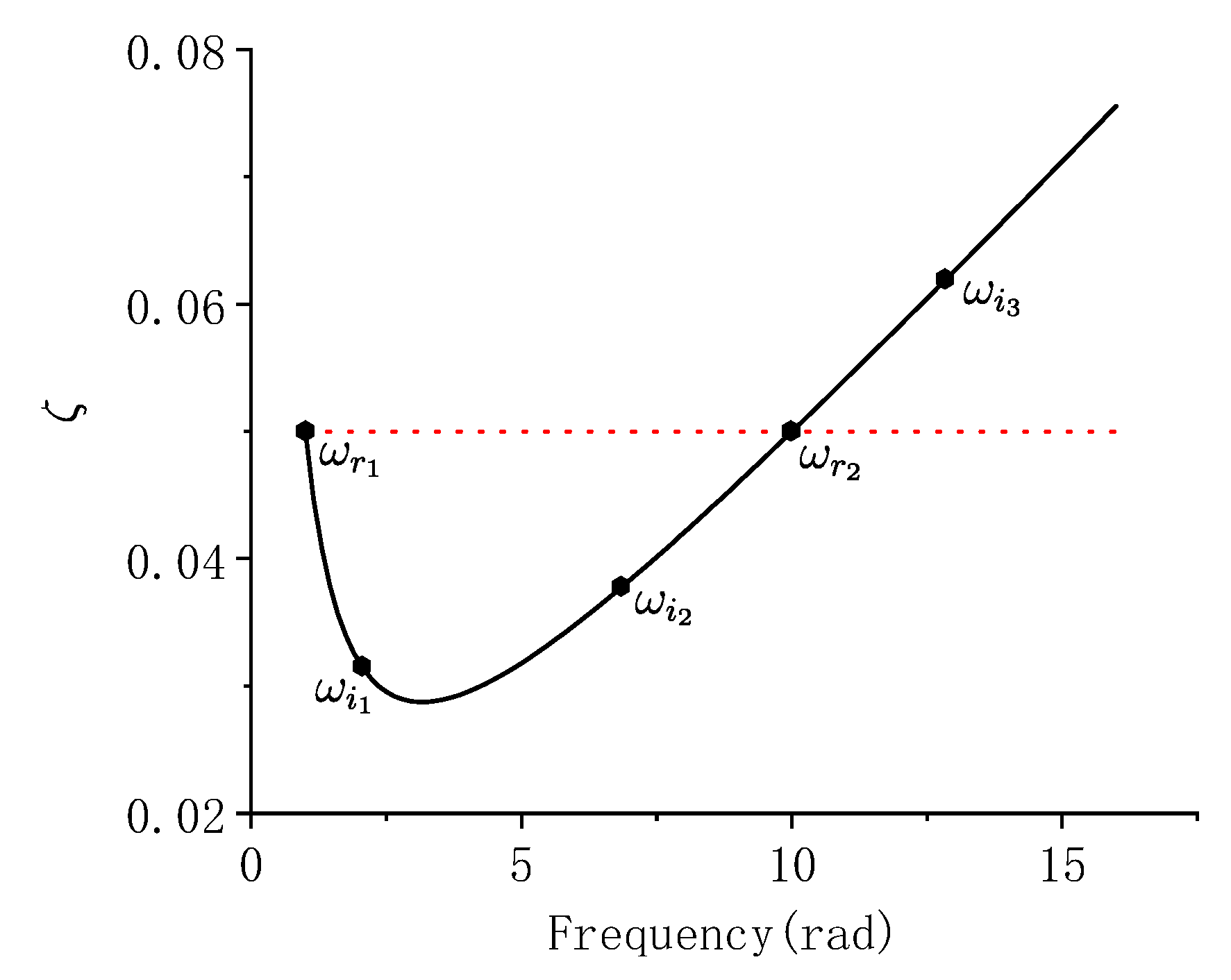
The damping ratios of the other modes are ${\alpha }_0/2{\omega }_i+{\alpha }_1{\omega }_i/2$. The first mode of the structure is usually chosen as ${\omega }_{r_1}$; the modes whose natural frequency larger than ${\omega }_{r_2}$ would have a damping ratio larger than $\zeta$ so that the energy of these modes is underestimated. Therefore, ${\omega }_{r_2}$ is chosen carefully that the underestimation of these modes would not significantly affect the result. For this reason, in this paper, only the damping truncation error of the modes whose natural frequencies are between ${\omega }_{r_1}$ and ${\omega }_{r_2}$ are analyzed. The relationship among ${\omega }_{r_1}$, ${\omega }_{r_2}$ and the natural frequency of some of the modes are briefly depicted in Figure 1.

The smallest possible value is $\min \left({\zeta }_i^r\right)=2\zeta \sqrt{{\omega }_{r_1}{\omega }_{r_2}}/\left({\omega }_{r_1}+{\omega }_{r_2}\right)$, when ${\omega }_i=\sqrt{{\omega }_{r_1}{\omega }_{r_2}}$ and ${\zeta }_i^r$ is the damping ratio of the $i^{th}$ mode. Usually, the smallest value cannot be achieved.

Transforming the first row of Equation (7) into modal coordinates, the EOM is shown in Equation (15).

$${\ddot{y}}_i^{Lr}+{\alpha }_0{\dot{y}}_i^{Lr}+{\alpha }_1{\omega }_i^2{\dot{y}}_i^{Lr}+{\omega }_i^2{y}_i^{Lr}=\frac{1}{2}{\left\{{\Phi }_{ss}{}^T{K}_{sb}\right\}}_{i,*}{\ddot{Y}}_b+\frac{1}{2}{\alpha }_0{\left\{{\Phi }_{ss}{}^T{K}_{sb}\right\}}_{i,*}{\dot{Y}}_b.$$

(15)

To compare Equation (12) with Equation (15), a variable $z_i=y_i^{Lr}-y_i^{Lm}$ is defined to measure the error when the Rayleigh damping method is used in LMM. Defining another parameter,

$$\beta =\frac{({\alpha }_0+{\alpha }_1{\omega }_i^2)-2\zeta {\omega }_i}{{\alpha }_0}=\left(\frac{{\omega }_i}{{\omega }_1}-1\right)\left(\frac{{\omega }_i}{{\omega }_2}-1\right).$$

(16)

The error $z_i$ can be expressed in the frequency domain as follows.

$${\stackrel{⌢}{z}}_i=\left(\frac{1}{2}j{\alpha }_0\omega \frac{(\beta -1){\omega }^2+2j\zeta {\omega }_i\omega +{\omega }_i^2}{\left(-{\omega }^2+2j\zeta {\omega }_i\omega +{\omega }_i^2\right)\left(-{\omega }^2+j({\alpha }_0+{\alpha }_1{\omega }_i^2)\omega +{\omega }_i^2\right)}\right){\left\{{\Phi }_{ss}{}^T{K}_{sb}\right\}}_{i,*}{Y}_b.$$

(17)

where ${\stackrel{⌢}{z}}_i$ stand for the Fourier transform of $z_i$. Define ${\mu }_i={\omega }_i/{\omega }_{r_1}$ and $\nu ={\omega }_{r_2}/{\omega }_{r_1}$. In the vicinity of zero frequency,

$${z_i|}_{(0,ϵ)}\approx \frac{j\zeta \nu }{{\mu }_i^2\left(1+\nu \right){\omega }_{r_1}}\omega {\left\{{\Phi }_{ss}{}^T{K}_{sb}\right\}}_{i,*}{Y}_b,$$

(18)

where $ϵ$ is a small positive number. In Equation (18), the error transfer function at zero frequency is zero; the amplitude of this error increase with frequency $\omega$, and is negatively correlated to the fundamental frequency of the structure, ${\omega }_{r_1}$; the larger the damping ratio $\zeta$ is the larger the error is.

Define the error ratio $r_i^{Lr}=\left|\left({\stackrel{⌢}{y}}_i^{Lr}-{\stackrel{⌢}{y}}_i^{Lm}\right)/{\stackrel{⌢}{y}}_i^{Lm}\right|$. The value of $r_i^{Lr}$ at zero frequency is infinite, which attribute to the second term at the right-hand side of Equation (5). As shown in Equation (17), the error has a peak in the vicinity of the resonance frequency. The value at the resonance frequency is derived as follows,

$${r_i^{Lr}|}_{{\omega }_i}=\sqrt{{(1-{\eta }_i)}^2+\frac{4{\zeta }^2{\nu }^2}{{(\nu +{\mu }^2)}^2}},$$

(19)

where ${\eta }_i=\zeta /{\zeta }_i^r$, ${\eta }_i$ represents the multiple of the expected damping ratio over the damping ratio of mode $i$.

In Equation (19), for a particular structure, the first term in the square root symbol increases with the parameter ${\eta }_i$ and the second term decrease with $\mu$. The possible largest value of ${\eta }_i$ is shown in Equation (20), and is achieved in the mode having the smallest damping ratio.

$$\max ({\eta }_i)=\frac{1}{2\sqrt{\nu }}+\frac{1}{2}\sqrt{\nu }.$$

(20)

From Equation (19), the behavior of the peak of $r_i^{Lr}$ is complex, the natural frequency of the mode having the largest error is between ${\omega }_{r_1}$ and $\sqrt{{\omega }_{r_1}{\omega }_{r_2}}$. The largest value of $r_i^{Lr}$ is larger than the larger value in ${r_i^{Lr}|}_{{\omega }_i={\omega }_{r_1}}=2\zeta$ and ${r_i^{Lr}|}_{{\omega }_i=\sqrt{{\omega }_{r_1}{\omega }_{r_2}}}=\sqrt{{(1-\frac{1}{2\sqrt{\nu }}-\frac{1}{2}\sqrt{\nu })}^2+{\zeta }^2}$. Equation (20) also indicates that, for a particular structure, the larger the value of $\nu$ is the larger the error is. The value $\max (\eta )$ doesn’t have an upper limit, as a result, the error ratio ${r_i^{Lr}|}_{{\omega }_i}$ can be a very large value.

When $\omega$ approaches infinity ${r_i^{Lr}|}_{\omega \to \infty }=0$. It is obvious in Equation (17) that the error ratio would be smaller than ${r_i^{Lr}|}_{\omega ={\omega }_i}$ for the frequencies larger than the resonance frequency. As a consequence, the error ratio at resonance frequency is a preferable value to represent the error in LMM-R.

Table 2. Error ratio $r_i^{Lr}$ for different $\nu$ and $\zeta$.

$\mathit{\nu }$	${\mathit{r}}_{\mathit{i}}^{\mathit{L}\mathit{r}}$$(\mathit{\zeta }=\mathbf{0.02})$	${\mathit{r}}_{\mathit{i}}^{\mathit{L}\mathit{r}}$$(\mathit{\zeta }=\mathbf{0.04})$	${\mathit{r}}_{\mathit{i}}^{\mathit{L}\mathit{r}}$$(\mathit{\zeta }=\mathbf{0.06})$
$2$	0.064	0.073	0.085
$4$	0.251	0.253	0.257
$6$	0.429	0.431	0.433

shows examples of the value of ${r_i^{Lr}|}_{\omega ={\omega }_i=\sqrt{{\omega }_{r_1}{\omega }_{r_2}}}$ for different parameters.

In Table 2, $r_i^{Lr}$ increases with the increase of $\nu$ and $\zeta$; the influence of $\nu$ is more significant than $\zeta$. The error ratio can be as large as 43.3%. The value in Table 2 is a good reference for estimating the largest damping truncation error of a particular mode.

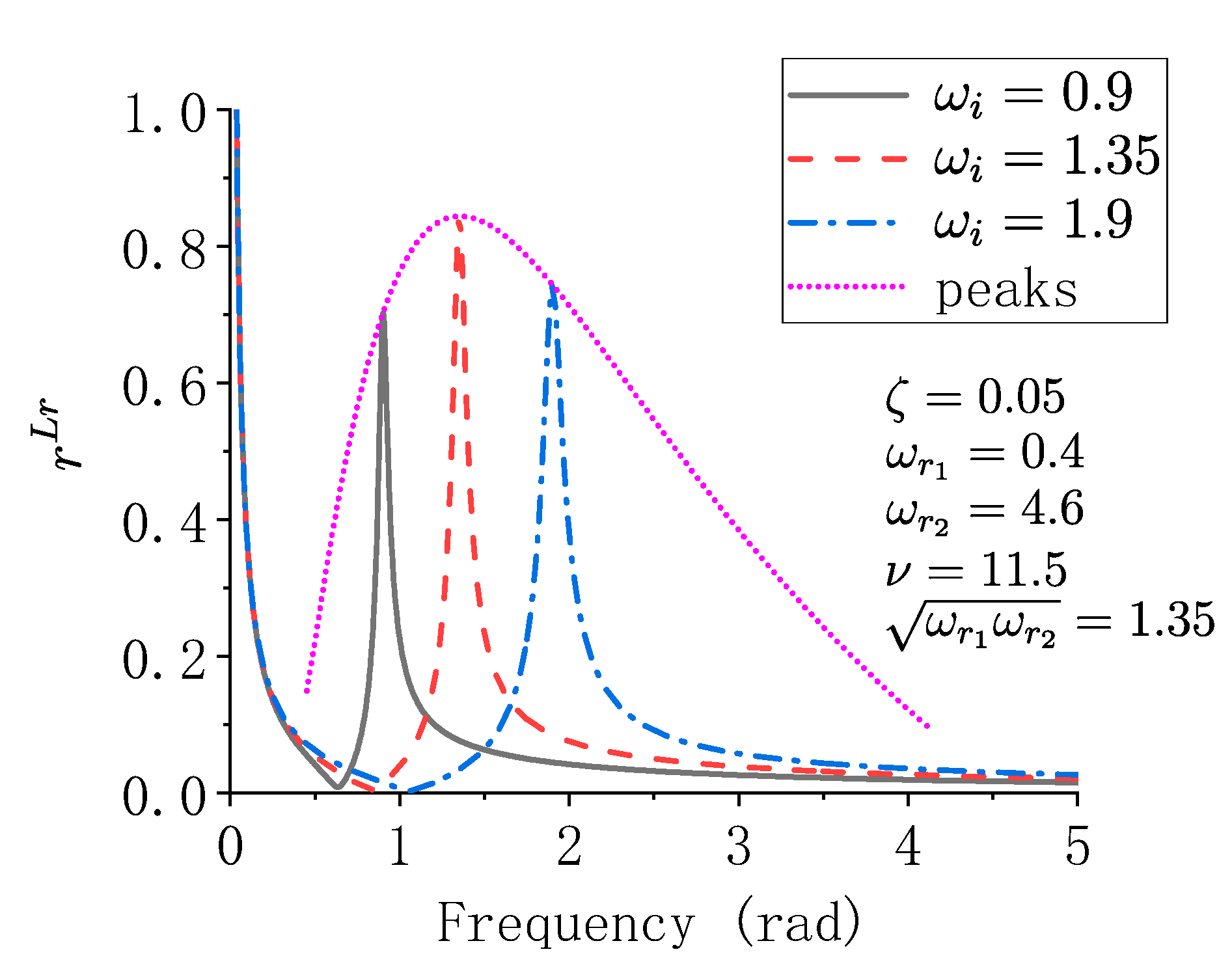
An example is demonstrated in Figure 2 showing the shape and the trace of peaks of $r_i^{Lr}$ when the mode has different natural frequencies.

In Figure 2, the large value of $r_i^{Lr}$ near 0 Hz is aroused by the second term at the right-hand side of Equation (15). As is analyzed, though the error ratio near 0 Hz is very large, the absolute value of error is small. The large value is the main component of virtual damping error in LMM-R. When $\omega$ < ${\omega }_i$, the error ratio decrease to zero at first. After that, the error ratio increase and reach its peak at the resonance point, showing that the influence of the large value around 0 Hz and the errors around the resonance point are separate. As analyzed before the peak of the error ratio reach is top when ${\omega }_i=\sqrt{{\omega }_{r_1}{\omega }_{r_2}}$, which is the main feature of the damping truncation error of the Rayleigh damping method.

Studies have shown that in the MSE problem, more modes need to be considered [15]. The damping truncation error might not be negligible in the MSE problem.

$$C\left(\begin{array}{c}{\Phi }_{sb}\\ {\Phi }_{bb}\end{array}\right)={\alpha }_0\left(\begin{array}{c}{M}_{ss}{\Phi }_{sb}+M_{sb}{\Phi }_{bb}\\ M_{bs}{\Phi }_{bb}\end{array}\right).$$

(21)

In LMM-R, the damping matrix $C$ does not satisfy Equation (10). This means that the damping truncation error of LMM-R contains the virtual damping error. At the end of the next subsection, another Rayleigh damping formula is introduced, that can eliminate virtual damping in LMM-R.

In the next subsection, using RMM with the Rayleigh damping method is proved free from virtual damping and has the same form as Equation (11). LMM has its advantage in time history study. The free-from virtual damping version of LMM can be easily derived from Equation (11). In this version, the Rayleigh damping is shown as follows.

$$C={\alpha }_0\left(\begin{array}{cc}{M}_{ss}& M_{sb}+{\tilde{M}}_{sb}\\ M_{bs}& \mathbf{0}\end{array}\right)+{\alpha }_1\left(\begin{array}{cc}{K}_{ss}& K_{sb}\\ K_{bs}& K_{bb}\end{array}\right);$$

(22)

where ${\tilde{M}}_{sb}=M_{ss}{K}_{ss}{}^{-1}{K}_{sb}$. With the help of ${\tilde{M}}_{sb}$, the second term at the right-hand side of Equation (15) is canceled. The EOM of the modal participation factor of mode i is shown as follows.

$${\ddot{y}}_i+{\alpha }_0{\dot{y}}_i+{\alpha }_1{\omega }_i^2{\dot{y}}_i+{\omega }_i^2{y}_i=\frac{1}{2}{\left\{{\Phi }_{ss}{}^T{K}_{sb}\right\}}_{i,*}{\ddot{Y}}_b;$$

(23)

Except for the damping ratio, the equation has the same form as Equation (12). With Equation (22), the EOM of LMM-R approaches RMM-R when the large mass approach infinity. With the help of Equation (22), the EOM of the LMM-R would have no virtual damping error but has only the damping truncation error inside.

3.2. Error in RMM

The way RMM solves the response of the structure guarantees that the EOMs derived with RMM does not contain virtual damping. In Appendix A, the following equation is proved.

$${\Phi }_{sb}\to R{\Phi }_{bb},$$

(24)

Equation (24) indicates that the mode shapes related to the relative motion of the supports are not affected by the mass distribution of the structure. This conclusion gives the physical meaning to separate the responses of the structure into pseudo-static responses and dynamic responses in RMM. Substituting Equation (24) and (4) into Equation (2), Equation (25) can be obtained.

$$Y_s^d=Y_s-{\Phi }_{sb}{\Phi }_{bb}^{-1}{Y}_b,$$

(25)

In Equation (25), the dynamic responses equal to subtracting the influence of the rigid body modes and the modes related to the relative motion of the supports from the total responses. In other words, RMM does not contain virtual damping.

To show this property of RMM in another aspect, put all the equations in RMM in a single equation. Adding Equation (4) to Equation (6) and transforming the result into absolute coordinates, the EOM of the absolute displacement is Equation (26).

$$M_{ss}{\ddot{Y}}_s+C_{ss}{\dot{Y}}_s+K_{ss}{Y}_s=-C_{sb}{\dot{Y}}_b-K_{sb}{Y}_b,$$

(26)

$C_{sb}=-C_{ss}R$ is assumed in the RMM. Equation (26) is the same as the one introduced by Qin et al. [8], which is derived from a modified LMM. The form of $C_{sb}$ in Equation (9) guarantees the establishing of Equation (10). The integrated EOM in Equation (26) is more efficient and can also be used in nonlinear analysis.

The above derivation proved that the assumption in RMM that $C_{sb}+C_{ss}R=\mathbf{0}$ will not induce the virtual damping error regardless of the damping formulating method.

But using the Rayleigh damping method would induce the damping truncation error in the calculation. Transforming Equation (26) into modal coordinates, the dynamic equation for the modal participation vector is shown in Equation (27).

$${\stackrel{⌢}{y}}_i^R=\frac{-2j{\zeta }_i{s}_i-1}{2(-s_i{}^2+2j{\zeta }_i{s}_i+1)}{\Phi }_{ss}{}^T{K}_{sb}{Y}_b,$$

(27)

where $s_i=\omega /{\omega }_i$, $y_i^R$ is the modal participation factor of mode $i$ and ${\stackrel{⌢}{y}}_i^R$ is the Fourier transform of $y_i^R$; ${\zeta }_i$ is the damping ratio this mode. the damping truncation error is measured with error ratio $r_i^{Rr}$, the EOM derived with RMM-M is used as the reference. When $s_i=1$,

$${r_i^{Rr}|}_{s_i=1}={\left|\frac{{\stackrel{⌢}{y}}_i^{Rr}-{\stackrel{⌢}{y}}_i^{Rm}}{{\stackrel{⌢}{y}}_i^{Rm}}\right|}_{s=1}=\frac{1}{\sqrt{4{\zeta }^2+1}}\left|{\eta }_i-1\right|;$$

(28)

The superscripts $Rm$ and $Rr$ represent the modelling method RMM-M and RMM-R, respectively. In Equation (28), when $\zeta$ is small enough, it has little influence on ${r_i^{Rr}|}_{s_i=1}$; ${r_i^{Rr}|}_{s_i=1}$ increases with $\eta$; the largest value of ${r_i^{Rr}|}_{s_i=1}$ is obtained in the mode whose natural frequency is the closest to the frequency $\sqrt{{\omega }_{r_1}{\omega }_{r_2}}$.

When $s_i=2$,

$${r_i^{Rr}|}_{s=2}=\frac{16\left|{\zeta }_i^r-\zeta \right|}{\sqrt{(16{\zeta }_i^r{}^2+9)(16{\zeta }^2+1)}}\approx \frac{16}{3}\zeta \left|\frac{1}{{\eta }_i}-1\right|;$$

(29)

When $s$ approaches infinity,

$${r_i^{Rr}|}_{s\sim \infty }\to \left|\frac{1}{{\eta }_i}-1\right|.$$

(30)

The larger ${\eta }_i$ is, the larger the error is.

For a particular mode, the error ratio decreases rapidly from the resonance frequency and then increases gradually as $s$ approach infinity. The increasing rate is very small, ${r_i^{Rr}|}_{s_i=1}$ is a good reference to the magnitude of the damping truncation error in RMM-R.

Table 3. Error ratio $r_i^{Rr}$ for different $\nu$, $\zeta$ and $s_i$.

$\mathit{\nu }$	$\mathit{\zeta }$	${\mathit{r}}_{\mathit{i}}^{\mathit{R}\mathit{r}}$$({\mathit{s}}_{\mathit{i}}=\mathbf{1})$	${\mathit{r}}_{\mathit{i}}^{\mathit{R}\mathit{r}}$$({\mathit{s}}_{\mathit{i}}=\mathbf{2})$	${\mathit{r}}_{\mathit{i}}^{\mathit{R}\mathit{r}}$$({\mathit{s}}_{\mathit{i}}=\mathbf{5})$
$2$	$0.02$	0.061	0.006	0.012
	$0.05$	0.060	0.015	0.027
$4$	$0.02$	0.250	0.021	0.041
	$0.05$	0.249	0.052	0.093

shows the error ratio for different parameters.

It is obvious in Table 3 that the influence of $\nu$ is larger than $s_i$ and $\zeta$. For a particular structure, the more modes need to be considered the larger the error $r_i^{Rr}$ is.

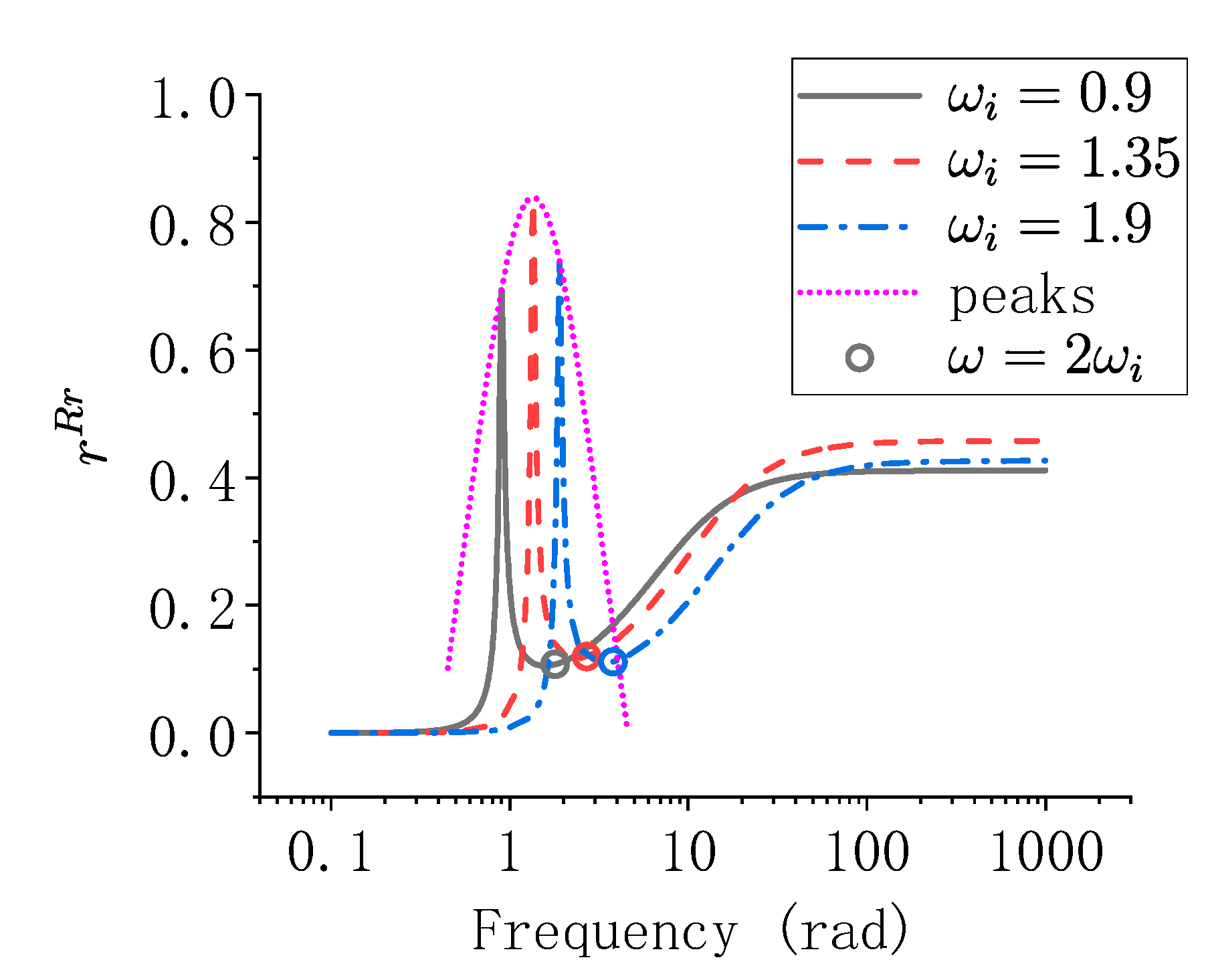
Figure 3 is an example used to show the feature of $r_i^{Rr}$ and its variation with the change of the modal natural frequency; the parameter settings are the same as Figure 2.

As is shown in Figure 3, $r_i^{Rr}$ has its first peak at the resonance frequency and the largest peak is acquired when ${\omega }_i=\sqrt{{\omega }_{r_1}{\omega }_{r_2}}$. When $\omega$>${\omega }_i$, $r_i^{Rr}$ decreases rapidly at first and gradually increases afterward, it finally arrives at a limit as shown in Equation (30). The largest value of the limit is also acquired when ${\omega }_i=\sqrt{{\omega }_{r_1}{\omega }_{r_2}}$. Though the limit error ratio can be very large, the absolute error is small. In Figure 3, the value of $r_i^{Rr}$ when $\omega =2{\omega }_i$ are marked with a circle on each line, at these points the value of the modal frequency response function has reduced to 1.9% of its resonance peak; and the value of the modal frequency response function is monotonously decreasing until infinity.

3.3. Error in ADM

In this section, the error caused by ignoring support damping, i.e., the ADM, will be studied. Firstly, virtual damping error is studied.

Transforming Equation (8) into modal coordinates, the EOM of ADM is shown in Equation (31).

$${\stackrel{⌢}{y}}_i^A=\frac{-1}{2(-s^2+2j{\zeta }_{i}s+1)}{\Phi }_{ss}{}^T{K}_{sb}{Y}_b,$$

(31)

Firstly, the error ratio $r_i^{Am}$ is derived. When the modal damping method is used, it is shown in Equation (32)

$$r_i^{Am}=\left|\frac{{\stackrel{⌢}{y}}_i^{Am}(s_i)-{\stackrel{⌢}{y}}_i^{Rm}(s_i)}{{\stackrel{⌢}{y}}_i^{Rm}(s_i)}\right|=\sqrt{1-\frac{1}{4{\zeta }^2{s}_i^2+1}},$$

(32)

where the superscript $Am$ and $Lm$ represents the EOM derive by ADM-M and LMM-M respectively. When $s_i=0$, $r_i^{Am}=0$; when $s_i$ is small,

$${r_i^{Am}|}_{s_i\in (0,ϵ)}\approx 2\zeta s_i.$$

(33)

When $s_i$ approaches infinity, $r_i^{Am}\to 1$. The error ratio for different damping ratios and different $s_i$ is shown in

Table 4. Error ratio $r_i^{Am}$ for different $\zeta$ and $s_i$.

$\mathit{\zeta }$	${\mathit{s}}_{\mathit{i}}=\mathbf{1}$	${\mathit{s}}_{\mathit{i}}=\mathbf{2}$	${\mathit{s}}_{\mathit{i}}=\mathbf{3}$
0.02	0.040	0.080	0.119
0.05	0.100	0.196	0.287
0.08	0.158	0.305	0.433

.

As shown in Table 4 and Equation (33), the errors increase with the increase of frequency, and also increase with the damping ratio of the mode; the error ratio can be 10% at the resonance frequency when $\zeta =0.05$; when the natural frequency of the mode is smaller than the dominant frequency of the earthquake, the error can also be significant in the higher frequency range.

Figure 4 shows examples of $r^{Am}$ for modes with different natural frequencies, the parameter setting is the same as Figure 2.

As is shown in Figure 4, the shape of $r^{Am}$ is not related to ${\omega }_i$. $r^{Am}$ increases monotonously with the increase in frequency and finally approach 1 as the frequency approach infinity. The value of $r^{Am}$ in Figure 4 at the resonance points are marked with squares and the value of them are all 10.0%; the value of $r^{Am}$ when $\omega =2{\omega }_i$ are all 19.6%, these values are the same as predicted in Table 4 $r^{Am}$ is caused by neglecting support damping, and is one kind of virtual damping error.

The same as LMM-R, in ADM-R, both the virtual damping error and the damping truncation error exist at the same time.

The error ratio of ADM-R when $s_i=1$ is shown in Equation (34).

$${r_i^{Ar}|}_{s_i=1}={\left|\frac{{\stackrel{⌢}{y}}_i^{Ar}(s_i)-{\stackrel{⌢}{y}}_i^{Rm}(s_i)}{{\stackrel{⌢}{y}}_i^{Rm}(s_i)}\right|}_{s_i=1}=\frac{1}{\sqrt{4{\zeta }^2+1}}\left|{\eta }_i-1\right|,$$

(34)

The influence of $\zeta$ is small, ${r_i^{Ar}|}_{s_i=1}$ also achieves its possible maximum value when ${\omega }_i=\sqrt{{\omega }_{r_1}{\omega }_{r_2}}$; when $s_i=2$, ${r_i^{Ar}|}_{s_i=2}$ increases linearly with $\zeta$, and increases with the increase of $\eta$.

$${r_i^{Ar}|}_{s_i=2}=4\zeta \sqrt{\frac{{(-4{\eta }_i+1)}^2+16{\zeta }^2}{(16{\zeta }^2+9{\eta }_i{}^2)(16{\zeta }^2+1)}}\approx \left|\frac{16}{3}-\frac{4}{3{\eta }_i}\right|\zeta ,$$

(35)

When $s_i$ approaches infinity, ${r_i^{Ar}|}_{s_i\to \infty }$ approaches 1.

Table 5. Error ratio $r_i^{Ar}$ for different $\nu$ and ${\omega }_i$.

$\mathit{\nu }$	$\mathit{\zeta }$	${\mathit{r}}_{\mathit{i}}^{\mathit{A}\mathit{r}}$$({\mathit{s}}_{\mathit{i}}=\mathbf{1})$	${\mathit{r}}_{\mathit{i}}^{\mathit{A}\mathit{r}}$$({\mathit{s}}_{\mathit{i}}=\mathbf{2})$
$2$	$0.02$	0.061	0.081
	$0.05$	0.060	0.200
$4$	$0.02$	0.250	0.085
	$0.05$	0.249	0.209

shows the value of $r_i^{Ar}$ for different parameters.

In Table 5, the value of ${r_i^{Ar}|}_{s_i=2}$ can be larger than ${r_i^{Ar}|}_{s_i=1}$, indicating that for structures having natural frequencies smaller than the dominant frequency of the excitation, the error caused by the excitation can be larger than the error caused by resonance response. The influence of $\nu$ is more significant than $\zeta$ at resonance frequency, whereas the influence of $\zeta$ is significant when $s_i=2$.

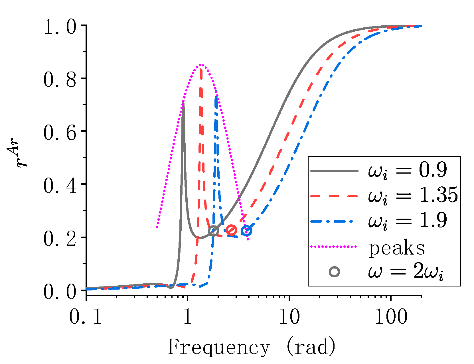
Figure 5 shows the features of $r^{Ar}$, the parameter setting is the same as Figure 2.

As is shown in Figure 5, the main features of $r^{Ar}$ are the combination of $r^{Am}$ and $r^{Rr}$. $r^{Ar}$ is the joint result of virtual damping error and damping truncation error. The largest value of $r^{Ar}$ when $\omega ={\omega }_i$ is slightly larger than that of $r^{Rr}$; the values of $r^{Ar}$ when $\omega =2{\omega }_i$ are all a bit smaller than $r^{Am}$ but around 8% larger than $r^{Rr}$.

4. Damping Formulating Error in MSE Problem

In the previous section, the virtual damping error and the damping truncation error that exist in the FRF of the modal participation factors are studied. In this section, a spectral analysis is used to demonstrate how the effect of MSE affects the accuracy of the structural responses is studied. The spatially variate ground motion is simulated as a random process, this method has been used by many researchers to study the effect of MSE.

The elements in the power spectral density (PSD) matrix of the excitation are usually described as follows.

$$S_{e,ij}(\omega )={\gamma }_{ij}(\omega )\sqrt{S_{e,ii}(\omega )S_{e,jj}(\omega )}$$

(36)

where $S_{e,ij}$ is the cross power spectral density function between the ground displacement $x_i$ and $x_j$. ${\gamma }_{ij}$ is the coherence function for $x_i$ and $x_j$.

$\left|{\gamma }_{ij}\right|$, which is the amplitude of the coherence function, usually named as lagged coherence [16] or incoherence effect [17], is represented by ${\gamma }_{ij}^l(\omega )$ in this study. The phase of ${\gamma }_{ij}$ is mainly composed of the wave passage effect, represented as ${\gamma }_{ij}^w(\omega )$, and site response effect describing the phase difference between different soil conditions, represented as ${\gamma }_{ij}^s(\omega )$. Kiureghian [17] proposed the following formula for describing ${\gamma }_{ij}$.

$${\gamma }_{ij}(\omega )={\gamma }_{ij}^l(\omega ){\gamma }_{ij}^w(\omega ){\gamma }_{ij}^s(\omega )={\gamma }^l(\omega )\exp [i({\theta }_{ij}^w(\omega )+{\theta }_{ij}^s(\omega ))]$$

(37)

The phases of the coherence function including the wave passage effect and the site-response effect are shown as follows.

$${\theta }_{ij}^w(\omega )=-T_{ij}\omega ,{\theta }_{ij}^s(\omega )={\theta }_j(\omega )-{\theta }_i(\omega )$$

(38)

where $T_{ij}={\eta }_{ij}{t}_{ij}$, describing the time for the ground motion to travel from support $i$ to $j$; $t_{ij}=d_{ij}/v_p$ is the time delay parameter, $d_{ij}$ is the distance between support $i$ and $j$, $v_p$ is the apparent propagation velocity of the earthquake; ${\eta }_{ij}$ is a coefficient describing the incident angle of the ground motion, $-1\le {\eta }_{ij}\le 1$; $T_{ij}$ is a universal coefficient describing the influence of both $v_p$ and ${\eta }_{ij}$; ${\theta }_i(\omega )$ is the phase of the local soil filter at support $i$.

Then, the PSD of the absolute displacement responses in modal coordinates is derived. To better illustrate how different factors of MSE affect the structural responses, the soil conditions at different structure supports are assumed to be the same. The PSD of the concerned responses can be derived as follows [1].

$$S_{y_i}(\omega )=S_g{\left|f_{y_i}\right|}^2\left[{\displaystyle \sum _{j=1}^{n_s}{q}_{ij}{}^2}+2{\displaystyle \sum _{j<k}{q}_{ij}{q}_{ik}{\gamma }_{jk}^l\cos \left(T_{jk}\omega \right)}\right]$$

(39)

$f_{y_i}=\frac{-2j{\zeta }_i{s}_i-1}{2(-s_i{}^2+2j{\zeta }_i{s}_i+1)}$; $S_g(\omega )$ is the spectral density function of the ground, $S_{y_i}$ is the PSD of the concerned modes $y_i$; $q_{ij}$ are constant coefficients.

When MSE is not considered, the PSD ${\hat{S}}_{y_i}$ of $y_i$ for the corresponding uniform excitation problem is.

$${\hat{S}}_{y_i}(\omega )=S_g{\left|f_{y_i}\right|}^2\left[{\displaystyle \sum _{j=1}^{n_s}{q}_{ij}{}^2}+2{\displaystyle \sum _{j<k}{q}_{ij}{q}_{ik}}\right]$$

(40)

Ripples with decreasing amplitude can be observed in Equation (39) because of the decaying parameter ${\gamma }_{jk}^l$ of the incoherence effect and the cosine function brought by the wave passage effect. With the help of these ripples, $S_{y_i}(\omega )$ vibrates around $S_g{\left|f_{y_i}\right|}^2{\displaystyle \sum _{j=1}^{n_s}{q}_{ij}{}^2}$. $q_{ij}$ can either be positive or negative, $S_{y_i}(\omega )$ can be significantly larger or smaller than ${\hat{S}}_{y_i}$. When the ridges of the ripples encounter the resonance peak, the amplitude of the resonance response will increase. As a result, the absolute value of the damping truncation error will increase. It is not easy to decide whether the influence of MSE has a positive or negative effect on reducing the virtual damping error and the damping truncation error.

The influence of wave passage effect including the influence of the structural span, the incident angle and the apparent propagation velocity of the ground motion is controlled by $T_{jk}$. When the value of $T_{jk}$ increases, the frequency of the cosine function increases, and the ripples are compressed inside the envelope formed by the incoherence effect. The peaks and troughs of the ripple interact with the resonant peaks of the structure and the energy peaks of ground motion, changing the shape of $S_{y_i}(\omega )$.

The coherence of the excitation decrease with the increase of the frequency. Thus, the incoherence effect controls the decreasing rate of the ripples’ envelope. When the coherence of the excitation approach zero, $S_{y_i}(\omega )$ approaches $S_g{\left|f_{y_i}\right|}^2{\displaystyle \sum _{j=1}^{n_s}{q}_{ij}{}^2}$, in this frequency range the higher modes that are not fully excited in the uniform excitation condition are significantly increased. At the same time, the errors at the resonance peaks would increase.

In the EOM of a structure, the magnitude of the virtual damping error depends on the magnitude of virtual damping in the structural model and the excitation amplitude in absolute coordinates.

Compared with the uniform excitation problem, in the MSE problem, the errors induced by the virtual damping and the damping truncation error have the following new features:

• The virtual damping error aroused by less compensated support damping would increase when the amplitude of the excitations in absolute coordinates are larger than their amplitude in relative coordinates.
• The interaction of ripples with the resonance peak of the structure can either increase or decrease the damping truncation error and the virtual damping error.
• The increase of the energy of higher modes due to the incoherence effect can either increase or decrease the damping truncation error and the virtual damping error.
• The requirement of considering more modes in the MSE problem can increase the damping truncation error.

5. Numerical Simulation

In this section, three cases are used to demonstrate the features of the virtual damping error and the damping truncation error and to show the influence of MSE on these two errors. The EOM of the structures are built with eight modeling methods namely LMM-R/M, RMM-R/M, ADM-R/M, and UN-R/M.

5.1. Cascaded Two Supports Multiple Degrees of Freedom Structure

Firstly, cascaded two supports multiple degrees of freedom structures are used to demonstrate the errors exist in the modal frequency response function.

In this part, concentrated multiple degrees of freedom mass-spring-damper systems are used in the numerical simulation to show the features of the virtual damping error and the damping truncation error in the FRF in modal coordinates. The error prediction formulas derived in the previous sections are testified. A sketch drawing of the structure is shown in Figure 6. In this model, n masses and n+1 springs are used.

In Figure 6, $m=1$ kg, the stiffnesses of the springs are 1 N/m. Rayleigh damping matrix is calculated with the first and the penultimate mode. The damping ratio of the structure is assumed to be 0.05. In the equation of motions derived in the previous section, the excitation coefficients are exactly the same. As a result, when the modal frequency response functions are studied, the form of excitation can only amplify the absolute value of the frequency response function but not the shape of it along the frequency axis. In this simulation, the excitations at the supports are assumed to be identical.

Different numbers of masses are used to study the influence of $\nu$ on the damping truncation error. The structure parameters of structures having different numbers of masses are shown in

Table 6. Parameters of the numerical simulations for structures with different number of degree of freedom.

n	${\mathit{\omega }}_{\mathbf{1}}$ (Rad)	$\mathit{\mu }$	$\mathit{\nu }$
5	0.518	1.93	3.35
10	0.285	2.92	6.74
15	0.196	2.96	10.01
20	0.149	3.94	13.23

. For each structure, the mode with the smallest damping ratio is used to calculate $\mu$ and $\nu$. These modes are also used for the calculation of the errors in the following context.

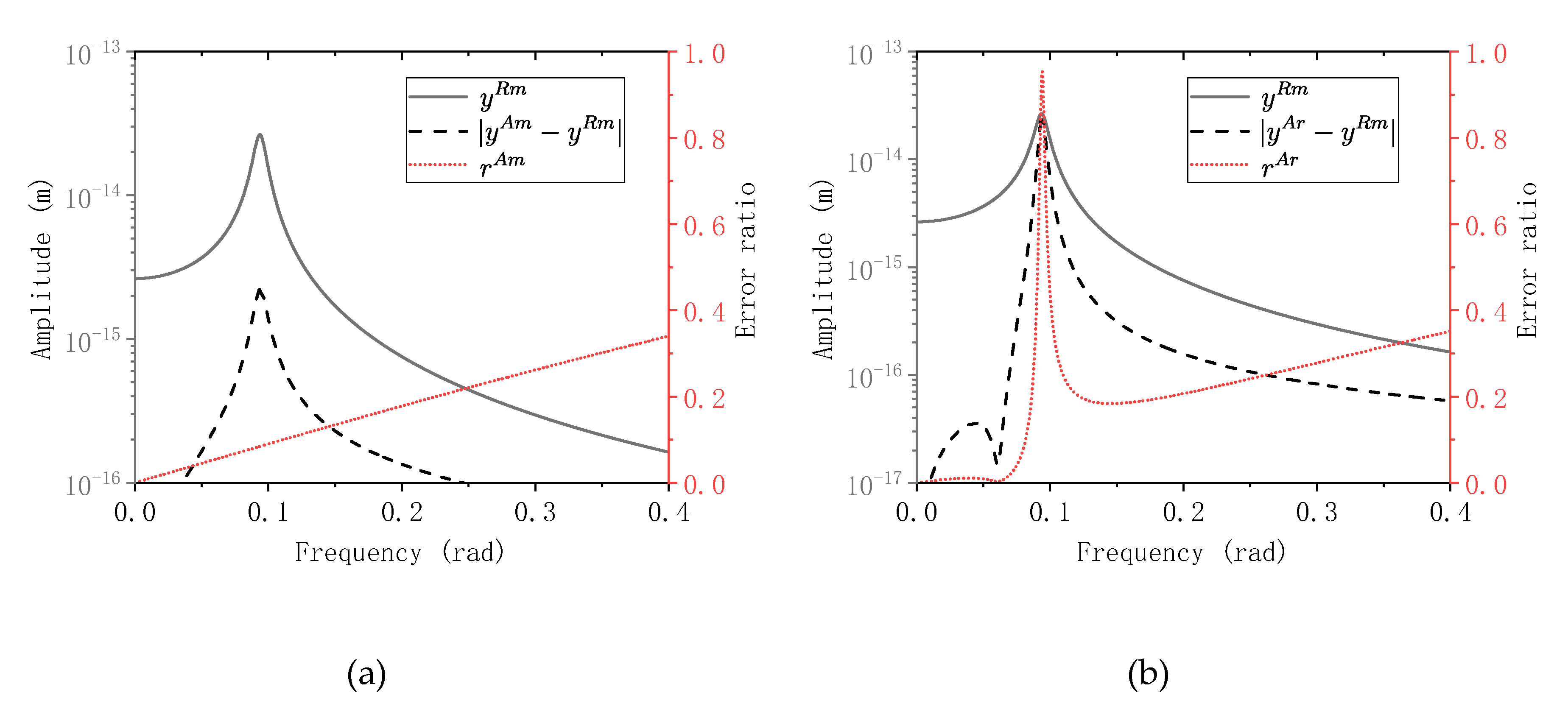
The Fundamental frequency of the structures decreases with the increase of the mass number; whereas $\mu$ and $\nu$ increases with it. Figure 7 shows the absolute errors and error ratios in the modal FRF of the 4th mode, when n = 20, and when LMM-R and RMM-R are use. The Rayleigh damping matrices are calculated with the 1st and the 19th mode.

As shown in Figure 7a, the input of this frequency response function is acceleration. The value of both the dashed line and the dotted line close to 0 Hz is significant showing the influence of the second term at the right-hand side of Equation (15). The error in this part is the main component of the virtual damping error in LMM-R. One peak of the error and error ratio appears at the resonance point. The shape of the dotted lines around the resonance point in Figure 7a,b are similar but with small differences, showing that the error in LMM-R near the resonance point contains little virtual damping error and is mainly composed of the damping truncation error. The varying trend of the error ratio is the same as predicted in the previous section. The largest value of the error ratio can be as large as 94% at the resonance point.

Figure 8 shows the errors and error ratios of ADM-R and ADM-M when n = 20.

As shown in Figure 8a, the varying trend of the dotted line can be approximated by a linear function which is predicted in Equation (33). The peak value of the dashed line, which is the absolute value of the error, also appears at the resonance point. In Figure 8b, the behavior of the error ratio is more complex than the other three models, multiple peaks appear in the dashed line; but the largest error ratio appears at the resonance point. In the frequency range $\omega$ > ${\omega }_4$, though the error ratio increases with the increase of frequency, the absolute value of the error decreases with frequency. Comparing Figure 8 with Figure 7, the errors in LMM-R and ADM-R are the joint effect of the virtual damping error and the damping truncation error. Neglecting support damping in ADM-M will induce the virtual damping error. The form of the virtual damping error in ADM-R and the damping truncation error in RMM-R are different. The virtual damping error in ADM-M can influence a wider frequency band and can arise a larger error in the energy of response; whereas the damping truncation error can cause large errors at resonance point.

In Figure 9a,b, the simulated value of the error ratios are compared with the theoretical results introduced in the previous section. Four structures with different numbers of masses are compared. The error ratios are measured at the resonance frequencies of the mode with the smallest damping ratio. The symbols ${\hat{r}}^{Lr}$, ${\hat{r}}^{Rr}$, ${\hat{r}}^{Am}$ and ${\hat{r}}^{Ar}$ are used, these symbols represent the estimated value of $r^{Lr}$, $r^{Rr}$, $r^{Am}$ and $r^{Ar}$. In Figure 9a, the error ratios in both the LMM-R and RMM-R increase with the increase of $n$, which reflects the increase in $\nu$. The results show the introduced formula performs well in approximating the error ratio. The error ratios in LMM-R and RMM-R are close to each other but have small differences.

In Figure 9b, as stated in the previous section, the error ratio $r^{Am}$ should not have related to the size of the structure. However, the simulation results show $r^{Am}$ changes slightly with the variation of n. For its reason, the error ratio of the numerical simulation is calculated at the resonance peak which is not the natural frequency of the undamped mode but close to it; the FRF changes rapidly in the vicinity of the resonance point contribute to the small variations. The error ratio $r^{Ar}$ also increases with n. The estimated error ratios show high accuracy compared with the simulation results.

5.2. 4-Span Rigid Frame Bridge

In this part, a 4-span bridge with a total length of 140 m is used to show the influence of MSE on the virtual damping error and the damping truncation error. The data of the bridge can be found in the reference [2]. Some of the data, including the span and height of the bridge, some of the node number and element number is shown in Figure 10. The frequency response function of the bridge beyond the 8th mode decreases rapidly and the energy of the ground motion is usually small after 10 Hz. Thus, in the analysis, the 1st mode and the 8th mode is used to calculate the Rayleigh damping matrix, and the damping ratio is assumed to be 0.04. A two-dimensional beam element is used as the element of this bridge.

Spectral analysis is used in this paper to show the statistical feature of the damping formulation problem. The spatially variate ground motions are simulated with stationary random processes.

As is shown in the previous section, LMM-M approaches RMM-M when the added large masses approach infinity. However, in LMM, a limited large number is practically assigned to the large masses instead of infinity. This process induces rigid body modes and modes with very low natural frequencies into the model. These modes do not actually exist in the real structure. If these modes were calculated in the responses, the responses will be overestimated. To study the error in LMM, a trick is indispensable. In this paper, the limit of FRF when the large masses approach infinity is used instead of the practical LMM. And ILMM is used to refer to this ideal LMM.

In this study, the soil conditions of the supports are assumed to be the same. The modified Kanai-Tajimi spectrum [1], which is also called the Clough-Penzien spectrum, is used as the spectral density function of the ground motion. The expression of this spectrum is shown in (41).

$$S_e=S_0\frac{{\omega }_g^4+4{\xi }_g^2{\omega }_g^2{\omega }^2}{{({\omega }_g^2-{\omega }^2)}^2+4{\xi }_g^2{\omega }_g^2{\omega }^2}\frac{1}{{({\omega }_f^2-{\omega }^2)}^2+4{\xi }_f^2{\omega }_f^2{\omega }^2}$$

(41)

Firm soil conditions are considered and the parameters are ${\omega }_g$ =15 rad, ${\omega }_f$ = 1.5 rad, ${\xi }_f$ = 0.6, ${\xi }_g$ = 0.6 Harichandran et al. [18]. $S_0$ represents the energy intensity of the ground motion. Peak ground acceleration of 0.5 g is used for determining the intensity of the ground motions. The mean peak value of the ground motion and the structural responses are calculated with the method introduced by Der Kiureghian [19]. The duration of the earthquake is assumed to be 20 s.

The model derived by Luco et al. [20] is used to describe the incoherence effect in Equation (37), the expression is shown in Equation (42).

$${\gamma }_{ij}^l=\exp [-{\left(\frac{{\lambda }_x\omega d_{ij}}{v_s}\right)}^2]$$

(42)

where $v_s$ is an estimation for the elastic S-wave velocity in the random medium, ${\lambda }_x=\mu \sqrt{R/r_0}$, $R$ is the distance in the random medium traveled by the wave; $r_0$ is the scale length of the random inhomogeneities along the path; ${\mu }^2$ is the measure of the relative variation of the elastic properties in the medium. The value ${\lambda }_x/v_s=2.5\times {10}^{-4}$ is recommended in the reference. [15]. The apparent propagation velocity of the ground motion is assumed to be 800 m/s. Existing researches have shown that the apparent propagation velocity is usually larger than 800 m/s.

The response PSD derived from different modelling methods are compared. The mean peak responses are used to measure the amplitude of responses.

A new error ratio is defined to measure the error of mean peak responses.

$$e^{Method}=\left|\frac{p^{Method}-p^{Rm}}{p^{Rm}}\right|,$$

(43)

where p stands for the mean peak responses; Method can be replaced by the name of different methods; the method RMM-M is used as the reference method.

The error ratios of all the displacement and force responses when using ILMM are smaller than ${10}^{-8}$ and are negligible, testifying to the conclusion that LMM approaches RMM when the large masses approaches infinity.

Table 7. Error ratio of responses when different modelling methods are used.

Responses	${\mathit{e}}^{\mathit{I}\mathit{L}\mathit{r}}$ (%)	${\mathit{e}}^{\mathit{R}\mathit{r}}$ (%)	${\mathit{e}}^{\mathit{A}\mathit{m}}$ (%)	${\mathit{e}}^{\mathit{A}\mathit{r}}$ (%)
$D_{n_3,2}$	0.14	1.02	−0.94	0.13
$D_{n_6,2}$	16.32	16.90	−0.55	16.30
$F_{e_3,5}$	0.02	0.97	−1.22	−0.14
$F_{e_7,5}$	3.81	4.02	−0.17	3.87
$F_{e_7,6}$	2.07	2.17	−0.15	2.10

listed the error ratio of several concerned responses.

In Table 7, the responses are represented as $D_{n_6,2}$ and $F_{e_3,5}$, the former one represents the vertical displacement of node 6; n in the subscript represents the node number; the latter stands for the shear force at the right end of element 3; e in the subscript represents the element number. The key nodes and elements are marked in Figure 10. The numbering of the degree of freedoms in the beam element is also shown in this figure. The numbering of the degree of freedoms in a node is the same as the left node in an element.

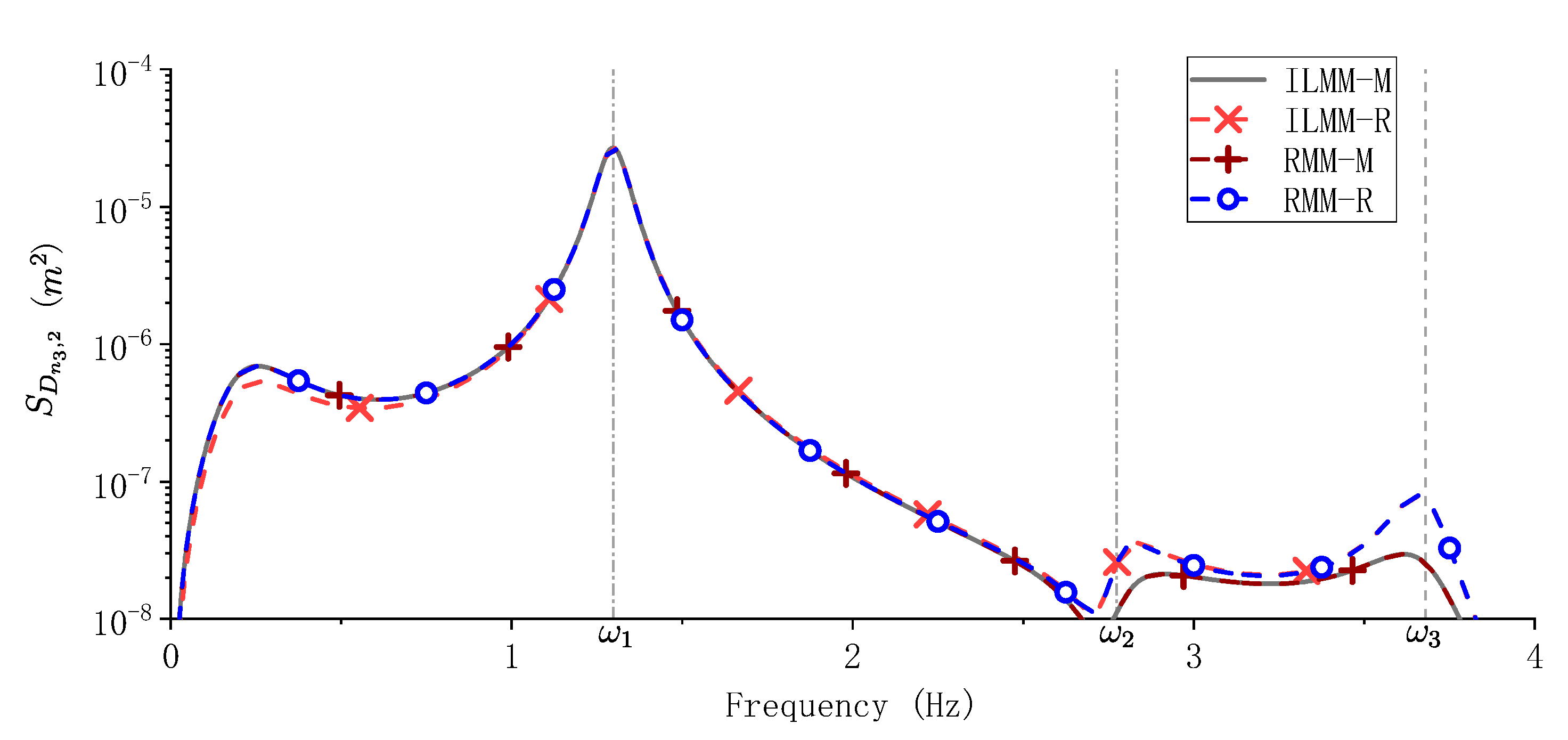
As is shown in Table 7, the error ratio of using the Rayleigh damping method in calculating the mean peak response of $D_{n_3,2}$ and $F_{e_3,5}$ are relatively small compared with the other responses. Figure 11 shows the PSD of $D_{n_3,2}$ derived with ILMM and RMM.

As is shown in Figure 11, the responses of ILMM-M and RMM-M overlap with each other testifying that these two modelling methods are equivalent. The response of RMM-R fit very well with RMM-M and starts to lose accuracy near the resonance peak of the 2nd mode, showing the influence of the damping truncation error. This phenomenon is also predicted in the previous derivation. The response of ILMM-R firstly shows an error at around 0.5 Hz, which attributes to the virtual damping error; the response of ILMM-R fit very well with the result of RMM-R showing that ILMM-R has both the virtual damping error and the damping truncation error. The response of $D_{n_3,2}$ is dominated by the responses before the natural frequency of the 1st mode, thus the influence of the damping truncation error is relatively small.

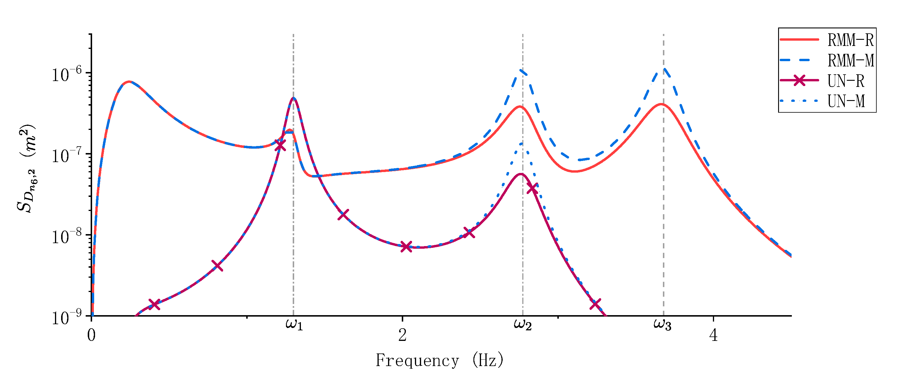
In Table 7, $D_{n_6,2}$ is obviously larger than the other responses. The response PSD of $D_{n_6,2}$ derived with the modelling methods RMM and UN are shown in Figure 12.

In Figure 12, the response PSD of $D_{n_6,2}$ at the 2nd mode and the 3rd mode is larger relative to the 1st mode, thus the influence of the damping truncation error on $D_{n_6,2}$ is larger than its influence on $D_{n_3,2}$. Compare the response of RMM and UN, under the influence of MSE the responses of the 2nd mode and the 3rd mode are obviously increased, which largely increases the damping truncation error.

In Table 7, the error of ADM-M can either be larger or smaller than the error ratio of RMM-R and ILMM-R showing that the influence of using the Rayleigh damping method can be larger than neglecting the support damping. The error ratio of ADM-R is a joint result of the virtual damping error and the damping truncation error.

5.3. Long Span Cable-Stayed Bridge

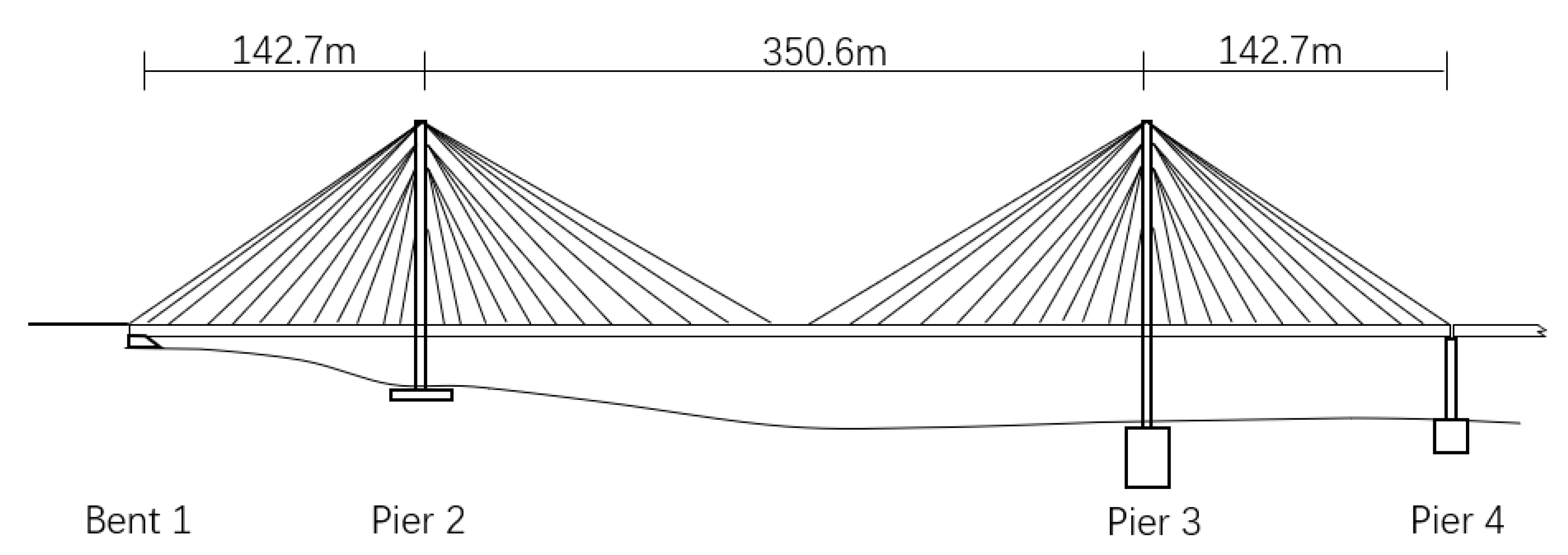
In the following context, the error in the modelling methods of a cable-stayed bridge is studied. The same analysis as the rigid frame bridge is carried out to this cable-stayed bridge. The bridge is introduced by Dyke et al. [21] and is used as a bench-mark bridge for control methods. The bridge is the Bill Emerson Memorial Bridge spanning the Mississippi River. A simplified drawing is shown in Figure 13. The detailed information of the bridge can be found in Dyke et al. [21]’s article and the data of the bridge can be found on the website [22].

The model of the bridge (see Supplementary Materials) is previously built for uniform excitation. In this paper, the model is rebuilt with the ‘hinged’ configuration as described in the files of the model. In the ‘hinged’ configuration, the deck is connected with the towers with shock transmission devices, which can be seen as rigid connections, the data can also be found in the reference. The stiffness matrix of the support is derived from the element stiffness matrices. The damping ratio of the bridge is assumed to be 0.03. The 1st and the 23rd mode are used for the formulation of the Rayleigh damping matrix. The responses under the excitation of ground motions from the longitudinal direction are studied. The soil conditions of the Piers are all assumed to be firm soil, and the energy intensity of the ground motion is decided with the same method as the rigid frame bridge.

Table 8. Error ratios of the mean peak responses of the responses of cable-stayed bridge.

Forces	Symbol	${\mathit{e}}^{\mathit{R}\mathit{r}}$ (%)	${\mathit{e}}^{\mathit{I}\mathit{L}\mathit{r}}$ (%)	${\mathit{e}}^{\mathit{A}\mathit{m}}$ (%)	${\mathit{e}}^{\mathit{A}\mathit{r}}$ (%)
Pier 2
Base shear	$F_{b,2}$	−3.64	−4.05	−8.63	473.91
Shear at deck level	$F_{d,2}$	−9.09	−8.88	−0.07	−9.15
Base Moment	$M_{b,2}$	−1.44	−2.14	−4.54	−4.40
Moment at deck level	$M_{d,2}$	−3.31	−3.08	−0.12	−3.22
Pier 3
Base shear	$F_{b,3}$	−3.80	−3.01	18.35	503.38
Shear at deck level	$F_{d,3}$	−16.15	−15.93	0.91	−16.23
Base Moment	$M_{b,3}$	−1.66	−1.04	5.21	56.43
Moment at deck level	$M_{d,3}$	−5.16	−4.68	1.46	−4.83
Cable forces
Largest Cable force	$F_c$	−3.42	−3.64	−0.28	−3.73

listed the error ratios of the mean peak value of several key responses.

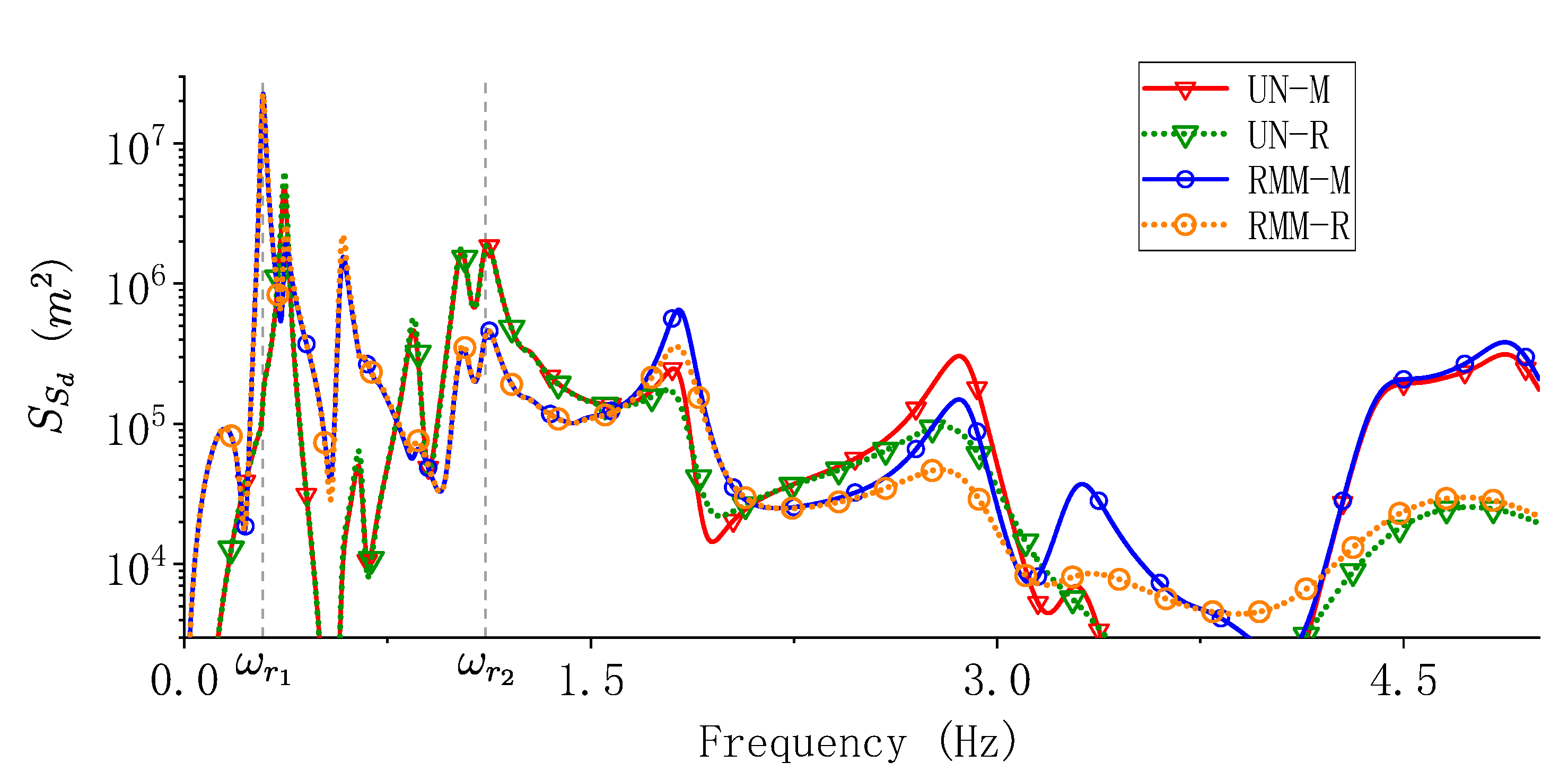
In Table 8, generally, the error ratio of the cable-stayed bridge is larger than that of the short span rigid frame bridge. The largest damping truncation error of RMM-R can reach 16.15%. The “hinged” model of the cable-stayed bridge assumes that the deck and the two towers of the bridge are perfectly connected, which will definitely increase the responses of the higher modes. Figure 14 shows the response PSD of $F_{d,3}$ when UN and RMM are used for modelling.

As is shown in Figure 14, the higher modes up to 5 Hz has significant energy compared with the first few modes. When using the Rayleigh damping method, the damping ratio of the modes having natural frequencies higher than ${\omega }_{r_2}$ are larger than ${\zeta }_{r_2}$ and the resonance responses of these modes are largely suppressed. That is the reason that the error ratio of $F_{d,3}$ are large. In Figure 14, the PSD of UN-M model has smaller energy at around 4 Hz; however, the PSD of RMM-M has a significant response. This phenomenon is caused by the effect of MSE. In this case, the effect of MSE increases the damping truncation error.

To reduce the error of RMM-R in calculating the responses of $F_{d,3}$, using a larger value of ${\omega }_{r_2}$ can help. However, when ${\omega }_{r_2}$ increases, the damping ratio of the other responses will definitely increase. The choice of ${\omega }_{r_2}$ requires more delicate consideration.

In Figure 14, compared with the PSD of UN-M model, due to the influence of MSE, some of the resonance peaks in the PSD of RMM-M are increased and some are decreased. The errors in the UN-R model and the RMM-R model originated from different modes. Therefore, it is hard to decide whether the effect of MSE would increase the damping truncation error or not.

In Table 8, the error ratio of ADM-M and ADM-R have large values when base forces are calculated. The largest error ratio reaches 503%, which is unacceptable showing that the neglect of support damping could cause huge errors. Though the error ratios in ADM of the other responses are acceptable, ADM is not recommended in the applications of the MSE problem.

In this paper, the influence of the apparent propagation velocity of the ground motion is also studied. The influence of the incident angle has a similar effect with the apparent propagation velocity. Figure 15 shows the variation of the mean peak responses of the mid-tower displacement of Pier 2, $D_{m,2}$, with respect to the variation of $1/v_p$.

As is shown in Figure 15, the results of RMM-M and ILMM-M match well with each other. $v_p$ mainly influence the vibration frequencies of the ripples caused by the wave passage effect. The error ratios of the other methods either increase or decrease with the variation of $1/v_p$. $v^{method}$ is defined as follows to measure the error sensitivity of $v_p$.

$$v^{method}={\max }_{v_p}\left|e^{Method}\right|-{\min }_{v_p}\left|e^{Method}\right|,$$

(44)

Table 9. Maximum variation of the error ratio for different apparent propagation velocity.

Forces	${\mathit{v}}^{\mathit{R}\mathit{r}}$ (%)	${\mathit{v}}^{\mathit{I}\mathit{L}\mathit{r}}$ (%)
Pier 2
Base shear	0.94	1.36
Shear at deck level	0.95	1.09
Base Moment	0.34	0.49
Moment at deck level	0.62	0.80
Pier 3
Base shear	1.54	0.93
Shear at deck level	1.03	0.89
Base Moment	1.16	0.69
Moment at deck level	0.69	0.91
Largest Cable force	3.53	3.32

shows the maximum changes of the error ratios when $v_p$ changes from 800 m/s to infinity.

As is shown in Table 9, the value of $v^{Rr}$ and $v^{ILr}$ are mainly around 1%. The largest value is observed from the largest cable force, which is around 3.5%.

The influence of MSE on the error ratio is also studied. Three variables are defined as follows.

$$e^{Ur}=\left|\frac{p^{Ur}-p^{Um}}{p^{Um}}\right|,$$

(45)

$$r_a^R=\frac{extrem{e}_{v_p}\left(p^{Rr}-p^{Rm}\right)}{p^{Ur}-p^{Um}},$$

(46)

$$r_r^R=\frac{extrem{e}_{v_p}(e^{RMM-R})}{e^{UN-R}},$$

(47)

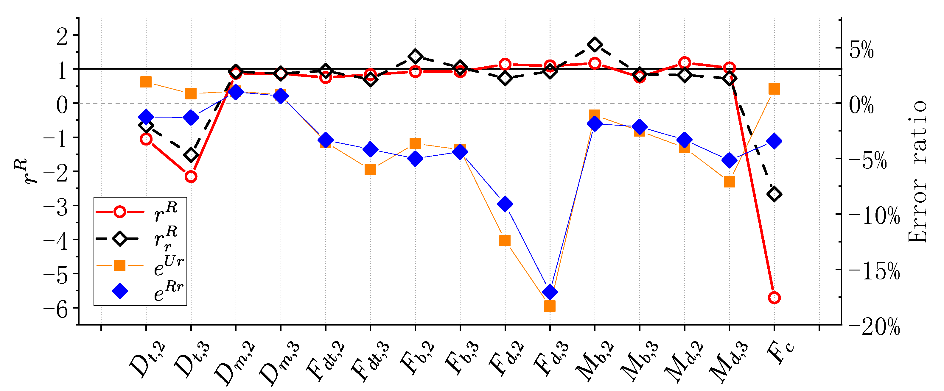
In Equation (46), $extrem{e}_{v_p}(p^{Rr}-p^{Rm})$ represents the extreme value of the damping truncation error of RMM-R when $v_p$ varies from 800 m/s to infinity. $e^{Ur}$ is used to measure the error ratio of the damping truncation error when uniform excitation is assumed. $r_a^R$ is used to measure the relative amplitude of the damping truncation error in the MSE problem and the damping truncation error of the corresponding uniform excitation problem; $r_r^R$ is used to measure the relative amplitude of error ratio of these two conditions.

Figure 16 demonstrates the influence of MSE on the damping truncation error. The error ratios of the key responses are compared in this figure.

In Figure 16, $D_{t,2}$ and $D_{t,3}$ represents the top tower displacement of Pier 2 and Pier 3, respectively; $D_{m,2}$ and $D_{m,3}$ are the mid-tower displacements; $F_{dt,2}$ and $F_{dt,3}$ are the axial forces of the deck-tower connection, the other notation can be found in Table 9. For most responses, the value of $r_a^R$ is around 1, in other words, the effect of MSE has little influence on the damping truncation error. However, for $D_{t,2}$ and $D_{t,3}$, which are the absolute displacements of the tower top, the error in MSE conditions changes to over two times its value in the UN condition; for $F_c$, the error in MSE condition changes more than times six times its value in the UN condition. Looking at the error ratio depicted in Figure 16, it is not hard to conclude that the amplitudes of the error ratios of $D_{t,2}$ and $D_{t,3}$ have little change except for their sign. The increase in the error is because of the increase in the absolute value of $p_{D_{t,2}}$ and $p_{D_{t,3}}$. $r_r^R$ shows the changes in error ratio consider or not the MSE, for $F_c$ the error ratio in MSE problem is still more than three times that of the uniform excitation problem. For the other responses, the error ratio can increase or decrease by more than 50%. MSE can affect the distribution of error, thus, can significantly increase the damping truncation error.

6. Conclusions

In this paper, the errors caused by virtual damping error and damping truncation error in the three modeling methods, the large mass method (LMM), the relative motion method (RMM), and the absolute displacement method (ADM), widely used in analyzing multiple support excitation (MSE) problems, are studied.

The term virtual damping is used to define the wrongly induced damping forces generated between the reference coordinates and the structure in the process of damping matrix formulation. The virtual damping error can be eliminated with the formula proposed in this paper. A new Rayleigh damping formula is proposed for LMM to eliminate the virtual damping error. With modal damping and the new Rayleigh damping formula, an integrated equation of motion (EOM) derived from the converged LMM is proved free from the virtual damping error and equivalent to RMM.

The damping truncation error is defined as the error caused by using Rayleigh damping instead of modal damping in the modelling of structures. The error in the structural frequency response function caused by the virtual damping error and the damping truncation error in the aforementioned three modeling methods are studied and the formulas measuring the largest error ratio are derived. The mechanism of how the effect of MSE affects the virtual damping error and the damping truncation error is studied by spectral analysis. A simplified mass-spring model, a short-span rigid-frame bridge and a long-span cable-stayed bridge are used for numerical simulation to testify the conclusions obtained in the theoretical derivation.

The following conclusions are acquired.

• RMM is free from the virtual damping error.
• When modal damping is used, the LMM converged to RMM. Using Rayleigh damping in LMM consists of both virtual damping error and the damping truncation error. When the newly-introduced Rayleigh damping equation is used in LMM, the LMM also converged to RMM and the virtual damping error in LMM is eliminated.
• The virtual damping error exists in all the structural modes of ADM. In ADM, the error ratio of the virtual damping increase with the frequency.
• The largest damping truncation errors in LMM, RMM, and ADM appear at the resonance frequency of the mode having the lowest damping ratio.
• For a particular structure, the damping truncation errors in LMM, RMM and ADM increase with the parameter $\nu$, which is the quotient of the two frequencies used in formulating the Rayleigh damping matrix.
• The effect of MSE changes the energy distribution among modes at the same time changes the distribution of error. Compared with the corresponding uniform excitation problem, the effect of MSE can either increase or decrease the virtual damping error and the damping truncation error in the model. The damping truncation error in the MSE problem can be significantly larger than the error in the corresponding uniform excitation problem.

References

1. Clough, R.W.; Penzien, J. Dynamics of Structures; Computers & Structures Inc.: Berkeley, CA, USA, 1995. [Google Scholar]
2. Leger, P.; Ide, I.; Paultre, P. Multiple-Support Seismic Analysis of Large Structures; Computers & Structures Inc.: Berkeley, CA, USA, 1990; Volume 36, pp. 1153–1158. [Google Scholar]
3. DebChaudhury, A.; Gazis, G.D. Response of MDOF systems to multiple support seismic excitation. J. Eng. Mech. 1988, 114, 583–603. [Google Scholar] [CrossRef]
4. Hall, J.F. Problems encountered from the use (or misuse) of Rayleigh damping. Earthq. Eng. Struct. Dyn. 2006, 35, 525–545. [Google Scholar] [CrossRef]
5. Chopra, A.K. Dynamics of Structures Theory and Application to Earthquake Engineering, 2nd ed; Prentice Hall: Upper Saddle River, NJ, USA, 2001. [Google Scholar]
6. Kabe, A.; Sako, B. Issues with proportional damping. AIAA J. 2016, 54, 2864–2868. [Google Scholar] [CrossRef]
7. Guo, W.; Yu, Z.-W.; Liu, G.-H.; Guo, Z. Possible existing seismic analysis errors of long span structures and bridges while utilizing multi-point earthquake calculation models. Bull. Earthq. Eng. 2013, 11, 1683–1710. [Google Scholar] [CrossRef]
8. Qin, H.; Li, L.; Spencer, B.F. Efficient Estimation of Seismic Response of Large-Span Structures Considering the Effect of Multiple-Support Excitation. J. Eng. Mech. 2019, 145, 04019096. [Google Scholar] [CrossRef]
9. Lanzi, A.; Luco, J.E. Caughey Damping Series in Terms of Products of the Flexibility Matrix. J. Eng. Mech. 2017, 143, 04017089. [Google Scholar] [CrossRef]
10. Luco, J.E. Explicit Representation of Classical Damping Matrices by Caughey Series with Rational Fractional Powers. J. Eng. Mech. 2017, 143, 06017008. [Google Scholar] [CrossRef]
11. Luco, J.E.; Lanzi, A. Optimal Caughey series representation of classical damping matrices. Soil Dyn. Earthq. Eng. 2017, 92, 253–265. [Google Scholar] [CrossRef]
12. Luco, J.E. A note on classical damping matrices. Earthq. Eng. Struct. Dyn. 2008, 37, 615–626. [Google Scholar] [CrossRef]
13. Kausel, E. Damping Matrices Revisited. J. Eng. Mech. 2014, 140, 04014055. [Google Scholar] [CrossRef]
14. Liang, Z.; Lee, G.C. Representation of Damping Matrix. J. Eng. Mech. 1991, 117, 1005–1019. [Google Scholar] [CrossRef]
15. Zerva, A. Spatial Variation of Seismic Ground Motions: Modeling and Engineering Applications; Crc Press: Boca Raton, FL, USA, 2016. [Google Scholar]
16. Jenkins, G.M.; Watts, D. Spectral Analysis and Its Applications; Holden-Day: San Francisco, CA, USA, 1968. [Google Scholar]
17. Kiureghian, A. A coherency model for spatially varying ground motions. Earthq. Eng. Struct. Dyn. 1996, 25, 99–111. [Google Scholar] [CrossRef]
18. Harichandran, R.S.; Hawwari, A.; Sweidan, B.N. Response of Long-Span Bridges to Spatially Varying Ground Motion. J. Struct. Eng. 1996, 122, 476–484. [Google Scholar] [CrossRef]
19. Der Kiureghian, A. Structural response to stationary excitation. J. Eng. Mech. Div. 1980, 106, 1195–1213. [Google Scholar]
20. Luco, J.; Wong, H. Response of a rigid foundation to a spatially random ground motion. Earthq. Eng. Struct. Dyn. 1986, 14, 891–908. [Google Scholar] [CrossRef]
21. Dyke, S.J.; Caicedo, J.M.; Turan, G.; Bergman, L.A.; Hague, S.T. Phase I Benchmark Control Problem for Seismic Response of Cable-Stayed Bridges. J. Struct. Eng. 2003, 129, 857–872. [Google Scholar] [CrossRef] [Green Version]
22. Dyke, S.; Agrawal, A.K.; Caicedo, J.M.; Christenson, R.; Gavin, H.; Johnson, E.; Nagarajaiah, S.; Narasimhan, S.; Spencer, B. NEES: Database for Structural Control and Monitoring Benchmark Problems. Available online: https://datacenterhub.org/resources/257 (accessed on 14 November 2020).
Figure 1. ω r 1 , ω r 2 and the natural frequency of the other modes in the Rayleigh damping method.
Applsci 10 08180 g001
Figure 2. Examples of r L r for a particular parameter setting.
Applsci 10 08180 g002
Figure 3. Examples of r R r for a particular parameter setting.
Applsci 10 08180 g003
Figure 4. Examples of r A m for a particular parameter setting.
Applsci 10 08180 g004
Figure 5. Examples of r A r for a particular parameter setting.
Applsci 10 08180 g005
Figure 6. Sketch drawing of the numerical model.
Applsci 10 08180 g006
Figure 7. Frequency response function of the 4th mode when n = 20, error and error ratio for different modeling methods, (a) large mass method with the Rayleigh damping method (LMM-R) (b) relative motion method with the Rayleigh damping method (RMM-R).
Applsci 10 08180 g007
Figure 8. Reference Frequency response function, error and error ratio for different modeling method (a) absolute displacement method with the modal damping method (ADM-M) (b) absolute displacement method with the Rayleigh damping method (ADM-R).
Applsci 10 08180 g008
Figure 9. Comparison of estimated error ratio and numerical results for different size of structures when different modeling methods are used, (a) r L r and r R r , (b) r A m and r A r .
Applsci 10 08180 g009
Figure 10. Simplified computational diagram of a 4-span rigid frame bridge.
Applsci 10 08180 g010
Figure 11. Comparison of the power spectral density (PSD) of D n 3 , 2 when ideal LMM-M (ILMM-M) and RMM-M are used.
Applsci 10 08180 g011
Figure 12. Comparison of the PSD of D n 6 , 2 when different modeling methods are used.
Applsci 10 08180 g012
Figure 13. Simplified drawing of Bill Emerson Memorial Bridge.
Applsci 10 08180 g013
Figure 14. Comparison of the PSD of S d , 3 when different modeling methods are used.
Applsci 10 08180 g014
Figure 15. The variation of the mean peak response of D m , 2 with respect to 1 / v p , when different modelling methods are used.
Applsci 10 08180 g015
Figure 16. Comparison of the damping truncation error for MSE problem and its corresponding uniform excitation problem.
Applsci 10 08180 g016