1. Introduction
Objective performance measurement is of great significance to the design and evaluation of audio systems. Commonly used indexes are signal-to-noise ratio (SNR), total harmonic distortion (THD), and signal-to-noise and distortion ratio (SINAD), and dynamic range (DR). They are interrelated and can be derived from each other [
1,
2]. For dynamic range performance evaluation, DR is an important index. However, the DR index in the existing literature does not show strictly consistent definitions and measurement conditions, which makes it difficult to achieve fair and effective performance comparisons between devices under test (DUTs). The DUT can be hardwares or algorithms.
To the best of the authors’ knowledge, there is no official or formal definition of the term DR. The “Standard method for digital audio engineering measurement of digital audio equipment” of Audio Engineering Society (AES) first defined its measurement as “
a comparison between the peak instantaneous sound levels occurring during a music performance and the just audible threshold for white noise when added to the program source” [
3]. Its latest version described DR as “
the ratio of the full-scale level at the output of the EUT to the weighted noise and distortion level in the presence of a low-level signal. It includes all harmonic, inharmonic, and noise components.” [
4]. Audio Precision stated that “
Dynamic range is the difference, usually expressed in decibels, between the highest amplitude signal which a device can output at its rated distortion, and the noise level of the device” [
5]. Other similar definitions of DR were given in [
6,
7,
8,
9,
10]. Moreover, it is stated that DR can be replaced by SNR if SNR’s measurement condition is 0 dBFS input [
3,
8], which means the implication of DR and SNR are consistent under this condition [
5]. However, the definition of SNR is still ambiguous for whether it includes harmonics and spurious. A direct description of “S/(N+D)” or “S/N” is clear but not convenient [
11].
Currently, the DR index is normally defined by a ratio; however, some details of the numerator and denominator have not been explicitly specified. They are listed as follows.
The noise floor, which has been discussed in detail in [
12]. The dominant view of noise floor calculation is to use the root-mean-square (RMS) amplitude of noise [
3,
4,
6,
7]. The harmonic, spurious and DC components are included in the noise calculation in [
4], and not included in [
12,
13]. This determines whether DR equals to SINAD or SNR under 0 dBFS input.
The maximal output. An instantaneous peak was used in [
3,
14], and an implied RMS peak was used in [
4,
6,
7].
The inconsistency of definitions and the ambiguity of details lead to differences between critical measurement conditions and schemes. Except for the different measurement conditions listed in [
6], other critical differences are as follows.
The amplitude of the testing signal. AES, IEC and EIAJ standards all use a −60 dBFS signal [
3,
4,
15,
16], and they are commonly used in [
17,
18]. But the amplitude is replaced by −40 dBFS in [
19].
The distortion degree. For example, “
rated distortion” was used in [
8], and “
often 1%” was expressed in [
5], and “
without distortion” was adopted in [
9,
10].
Then there are the measurement schemes. AES standard directly measures the ratio of the maximum of DUT output to the noise and distortion by a notch filter [
4,
19,
20]. IEC, EIAJ and Kester obtain DR by inverting the measured THD+N [
15,
16,
21]. Subtracting THD+N from THD to make the measurement results meaningful in the presence of a signal is used in [
19], because the noise floor is different when an input signal is absent or not.
In summary, the definition and measurement methods of DR are ambiguous in many respects. However, there are two main reasons why the results vary greatly. First, the degree of distortion is not clearly specified during the measurement. Generally, it is smaller for a lower amplitude of the testing signal. The current measurement condition specifies the test signal amplitude as −60 dBFS. However, in practice, distortion is inevitable, just to varying degrees. Therefore, the ultra-low amplitude measurement condition can neither match with the actual distorted working state of DUTs, nor extract its distortion behavior. Secondly, whether consider harmonic and spurious components. In fact, harmonics and spurious components are just different categories of distortion, and both of them can lead to performance degradation of DUTs. The DR in practice cannot avoid distortion. DR measurement should include all the noise, harmonic and spurious, which means DR equals SINAD in this paper. In addition, the SNR, THD, and SINAD indexes are often used together to evaluate the performance of DUTs, but there is a situation that the above indexes of the two DUTs are all equal or very close to each other. This leads to the difficulty of performance comparison. Therefore, an index that can overcome the ambiguities and shortcomings mentioned previously is necessary.
This paper proposes a new audio distortion dynamic range (ADDR) index as an effective complement to the existing indexes. The proposed ADDR can avoid both the ambiguity occurring in the DR by using the full-scale test signal condition and the controversy during practical use by clarifying that the calculation includes harmonic components in the definition of ADDR. Therefore, the uncertainty of measurement results and the false performance labels of manufacturers will be greatly reduced. Moreover, the ADDR index is novel in several ways. First, compared with the existing DR measurement methods, it is more practically applicable because its measurement conditions are closer to the actual distorted usage conditions. Secondly, the ADDR index unifies the SINAD and SNR indexes, and it can depict more subdivided performance between SINAD and SNR. Thirdly, the ADDR index comprehensively reflects the impacts of harmonic, spurious, and noise spectral components on DUTs. This helps to compare DUTs if the differences of the traditional indexes of DUTs are not obvious. Finally, as is widely known, automatic speech recognition (ASR) is one of the common applications of audio systems, and its accuracy is tightly related with the fidelity of the corresponding audio system, in this paper, the flexible simulated DUTs with the specified performance characteristics are adopted to verify the higher performance resolution of our ADDR index, as well as its supplementary function to the existing indexes, such as SNR, SINAD, and THD, those are commonly used in performance evaluation of an audio system.
The outline of this paper is as follows.
Section 2 describes the definition of the proposed ADDR index, to which the critical influence factors are addressed in
Section 3.
Section 4 reports several experiments to evaluate the proposed ADDR index, followed by the conclusion in
Section 5.
2. Definition of the New Index
The unwanted signals produced by a DUT will inevitably introduce distortion when a pure input signal goes through. Here the unwanted signals include the harmonic, spurious and noise components. The proposed ADDR index comprehensively depicts the process of how the dynamic range performance of the DUT is affected by these distorted signals, and the definition is as follows.
Audio Distortion dynamic range (ADDR): For a full-scale pure sine-wave input of a specified frequency, the ratio of the power of the DUT’s output averaged spectral component at the input frequency,
, to the power summation of distorted spectral components omitting those components above a threshold. The distorted spectral components are observed over a specified frequency band, and the range of the threshold is from the maximum of the magnitude of the distorted spectral components to the maximum of the magnitude of the noise spectral components:
where
is the averaged spectrum of the DUT output;
is the input signal frequency;
are the frequencies of the set of harmonic, spurious and noise spectral components, respectively. They are all within the specified frequency band;
is the threshold, whose range is from the maximum of to the maximum of ;
are the frequencies of the set of harmonic, spurious and noise spectral components that equal to or lower than the threshold , respectively.
The definition method between the existing indexes and the ADDR index is different. The SNR, SINAD, THD, and spurious-free dynamic range (SFDR) indexes are based on the ratio of the power of the fundamental signal to different categories of distorted spectral components. However, the ADDR index does not classify the distorted spectral components by treating them all as the unwanted signals. The definition of the ADDR index replaces classification with a variable threshold. The relative size of the threshold represents the distance from the magnitude of the fundamental signal. The ratio of the power of the fundamental signal to the distorted components at a fixed threshold describes the corresponding degree of signal headroom. The ADDR results corresponding to all the thresholds moving from the maximum to the minimum (ADDR plot) describes the changing process of the headroom degree from the relative worst to the relative best.
2.1. Obtain the ADDR Plot with the Spectrum
The input signal with the largest full-scale amplitude usually corresponds to the maximum distortion of the DUT, and the distortion behavior of the DUT can be extracted to the greatest extent. For a certain DUT, the ADDR equals to the SINAD and the SNR when the threshold equals to the maximum and the minimum of its range, respectively. Because the threshold in the ADDR definition is not fixed, the result of the ADDR index is a function of threshold, in which the ADDR changes monotonously. Moreover, the frequency response of the DUT is probably not flat, a more comprehensive measurement should be a function of frequency.
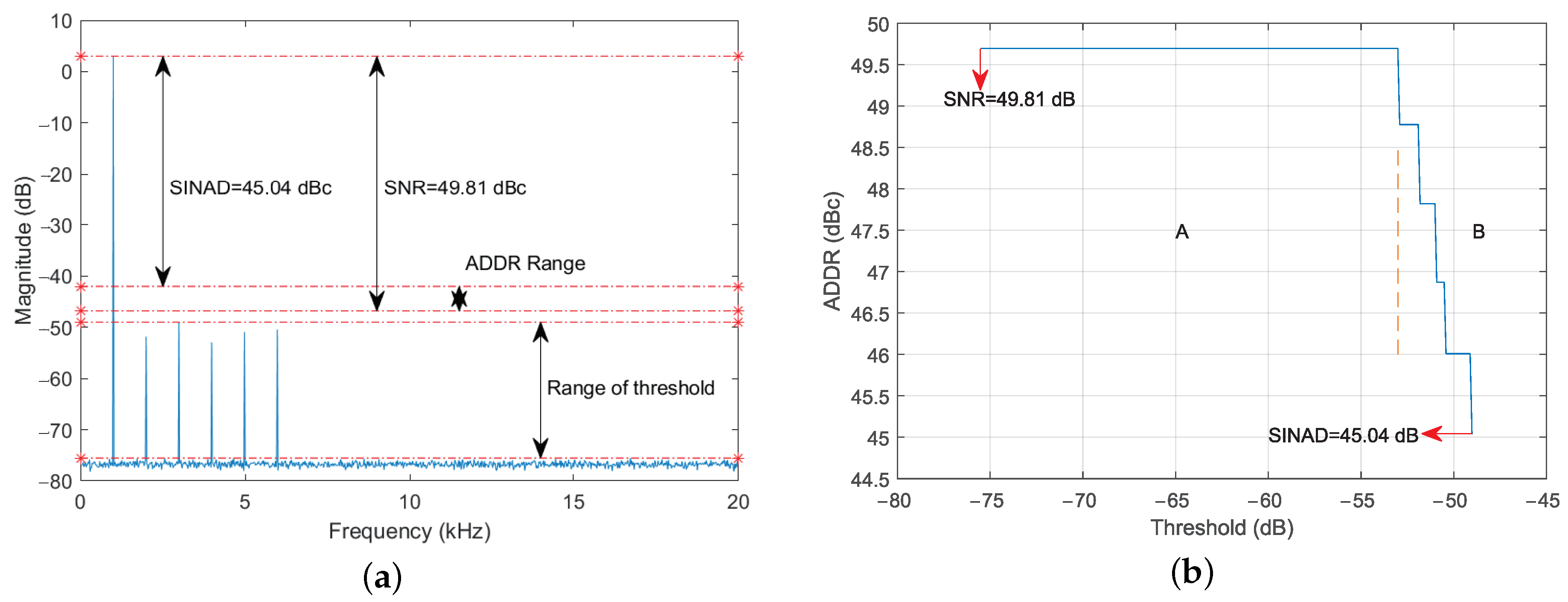
Take the averaged spectrum of a DUT’s output signal shown in
Figure 1a as an example, the detailed steps of obtaining the corresponding ADDR plot illustrated in
Figure 1b are as follows. Assume
is the averaged spectrum of the DUT output at frequency
f.
Step 1: Determine the span of the FFT bins of the fundamental signal of frequency f;
Step 2: Compute the power of the fundamental signal by the sum-of-squares of corresponding FFT bins: ;
Step 3: Set the minimum of threshold as the magnitude of the highest noise spectral component and the maximum threshold as the maximum magnitude of the distorted spectral component, respectively;
Step 4: Determine the step size sequence of the moving threshold: ;
Step 5: Initialize threshold as the maximum of distorted spectral components: T = ;
Step 6: Select the distorted spectral components that equal to or lower than threshold T;
Step 7: Compute the power summation of the selected distorted spectral components by the sum-of-squares of selected FFT bins: ;
Step 8: Compute the ADDR result corresponding to this specified threshold T: ;
Step 9: Decrease threshold T to in steps of corresponding , and repeat steps 6, 7 and 8 after each decrement to obtain the ADDR plot as a function of threshold of the DUT.
Figure 1a depicts that the range of the threshold is from the maximum of the harmonic, spurious components to the highest noise components. The ADDR of the DUT equals to the SINAD and the SNR when at its minimum and maximum, respectively.
Figure 1b verifies that the ADDR index unifies the SNR and SINAD indexes when at its two extremes. Moreover, the ADDR plot depicts a subdivision process of the distortion between the SNR and the SINAD. The dotted line separates the ADDR plot into part ‘A’ and ‘B’, part ‘A’ depends on the noises of the DUT while part ‘B’ depends on the harmonic and spurious components. The ADDR values between two ends are equivalent to multiple indexes similar to the SNR index. Thus, the ADDR plot is to a great extent a comprehensive depiction of the performance of the DUT.
Please note that the definition of ADDR only considers the power of distorted spectral components rather than the different influences of different frequencies for a certain target application. If necessary, it can be balanced by a weighting function multiplied on the spectrum. For example, if DUTs are compared from the perspective of end-users’ experience, psychoacoustic unevenness of distorted frequencies should be considered [
22].
2.2. Judgement Rules
Taking the comparison of two DUTs as an example, the ADDR plots of these DUTs are illustrated in
Figure 2a. There are two basic rules: (a) Corresponding to the same ADDR on the vertical axis, the smaller the value of the threshold on the horizontal axis is, the better the DUT performance is. This is reasonable because for a same ratio of signal to specified distorted spectral components, a lower threshold represents a larger clearance area near the fundamental signal. (b) Corresponding to a same threshold on the horizontal axis, the larger the value of the ADDR on the vertical axis is, the better the DUT performance is. Because for the same threshold a higher ADDR value represents a larger ratio of signal to specified distorted spectral components.
The ADDR plot reflects the process of performance variation from SINAD to DR caused by the distorted components of a DUT. Therefore, comparing the ADDR performance of two DUTs is achieved by comparing the area of the specified region of the ADDR plot. The smaller the area of the specified region of a DUT is, the better the performance of the DUT will be. The steps to obtain the area of the specified region are as follows, and they are correspond to each sub-figure in
Figure 2 respectively.
Step 1: Put the ADDR plots of the two DUTs in a figure;
Step 2: Specify the origin of the specified region as the intersection of the horizontal reference line whose vertical position is the biggest ADDR value and the vertical reference line whose horizontal position is the smallest threshold;
Step 3: Draw three reference lines. Start from the origin, draw a horizontal reference line and a vertical reference line to left and to down respectively. Draw a vertical reference line whose horizontal position corresponds to the biggest threshold of these DUTs;
Step 4: The area of the specified area is equal to the area formed after the ADDR curve directly intersects or projects its ends onto the reference lines.
Projecting the ADDR curve’s ends onto the reference lines is necessary because it prevents the area comparison rule from producing incorrect results based on the two basic rules in some cases and provide more flexibility.
For the DUTs with different maximum thresholds, projecting onto the right vertical reference line is equivalent to horizontally extending the ADDR plot of the corresponding DUT with a smaller minimum threshold in that direction. This is reasonable because in the spectrum if the position of the threshold is higher than the maximum of distorted components, the ADDR result is unchanged. The projection onto the left vertical reference line is to make the comparison process meet the set rules.
Figure 2d shows the comparison result, within which the reference lines are illustrated by the black lines. The origin is shown as the dot on the north-western region. The areas of the specified region of DUT1 and DUT2 are illustrated by the areas of ‘S1’ and ‘S2’, respectively. It is obvious that the area ‘S1’ is smaller than the area ‘S2’, thus, the overall ADDR performance of DUT1 is better than that of DUT2.
3. Critical Influence Factors
The proposed ADDR index is calculated in the frequency domain, and its basis is to obtain an accurate DUT output spectrum. Therefore, it is of great significance to ensure all the critical factors are controlled. They are leakage, windowing, number of sampling points, step size of the moving threshold and span of FFT bins of the specified signal.
3.1. Leakage
For an
N points finite sequence sampled at a sampling frequency of
. The DFT processing generates an
N point transformation, and the frequency corresponding to the output sequence is
The condition that DFT can correctly generate amplitude information is that the energy of the input data sequence is accurately included in the frequencies given by (
2) [
23]. In other words, the frequency of sampled signal
is at an integer multiple of the frequency resolution.
For a single sine signal input, the output of the DUT includes not only the fundamental signal, but also the unwanted harmonic, spurious and noise components. It is rather difficult to ensure that all signals do not have spectral leakage, but its influence on the ADDR index is different for each spectral component. Generally, the higher the power of the FFT bin is, the more obvious the effect of the FFT bin is. Because the proposed ADDR index uses a single pure sinusoidal test signal, the output power of the DUT is mainly concentrated at the input signal frequency and its harmonics, and the power of the noises is relatively much lower. Therefore, the leakage caused by the fundamental signal and its harmonics should be the focus of attention, and the leakage caused by the noises is negligible [
24].
The leakage can be reduced by various omethods [
25,
26,
27,
28,
29], which are mostly based on the estimation of fundamental frequency. However, the optimal measurement condition is to make the sampling process satisfy the requirement of coherent sampling for both the fundamental frequency and its harmonic frequencies simultaneously, which significantly increases the spectral resolution of the FFT and creates an ideal environment for critically ADDR performance evaluation of the DUT. The frequencies of the set of harmonics
are the integer multiples of the fundamental frequency
. Therefore, the condition making the fundamental wave satisfy coherent sampling also ensures that the harmonics meet the coherent sampling condition. The coherent sampling of a pure single sine test signal occurs when the number of cycles in the sampling window is an integer.
where
M is the integer number of cycles in the data records. Although the coherence relationship is applicable to any
M and
N, the optimized choice of
M and
N can further improve the accuracy and the computational complexity. First, the optimized value of
N is a power of 2 because of the inherent periodicity of FFT. Secondly, the optimized value of
M is an odd or prime, which can eliminate part even all the common factors of
N. This is because the common factors between
M and
N lead to different harmonics of
in the same frequency bin during the FFT after aliasing [
23].
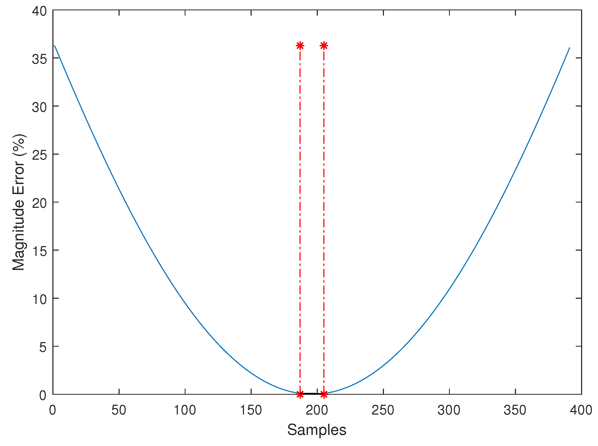
The magnitude accuracy of the fundamental signal is highly related to the accuracy of the ADDR plot.
Figure 3 shows the leakage effect on the magnitude error percentage for a shift in
M from
M− 0.5 to
M + 0.5. In practice, these shifts of
M represent an input frequency range from about 986 Hz to about 1006 Hz.
The vertical axis error percentage is the result of the corresponding horizontal axis changing from M− 0.5 to M + 0.5. Since the signal magnitude is known, the optimal condition is to achieve 0% magnitude error. Indeed, the minimum of the magnitude error achieves 0.0002% only when the frequency is close to 996.1 Hz. The maximum percentage of the magnitude error is more than 35%, and only the samples of M between the very slim region formed by these two dotted lines achieves a magnitude error percentage smaller than 0.1%.
In summary, the ADDR index is very sensitive to the leakage. For the ADDR measurement of single input frequency, the ideal condition of ADDR measurement is to compute a sampling frequency that results in an equivalent ratio
(
M is odd or prime) that is rational, and tune the sampling frequency to the computed frequency, then the leakage can be minimized by using a Kaiser window with parameter
= 0 [
30].
3.2. Windowing
To measure ADDR as a function of frequency, the specified frequency band is fixed, for example 20 kHz for audio DUTs. It is hard to guarantee the process of ADDR measurement satisfies the optimal coherent sampling condition for all the frequencies, then windowing operation improves the measurement accuracy. Kaiser windows are the most recommended to be used in the proposed ADDR measurement in this situation.
Kaiser window controls the proportion of the signal energy captured by the mainlobe mainly through an adjustable shape factor,
[
31]. The shape factor ranges from
= 0 to
= 40. The minimum
is equivalent to a rectangular window and the maximum
offers a wide enough mainlobe capturing the vast majority of the spectral energy representable in double precision. Moreover, a typical intermediate value of
6 approximates a Hanning window closely. Thus, the value selection of
is of great significance, which depends on the actual spectrum of the DUT. If the test satisfies the coherent sampling conditions for the fundamental signal,
should be set as 0; If the spectral resolution is very critical, which means there exists spurious very close to the fundamental signal,
should be small; If the spurious and harmonics are far from the fundamental from the spectral resolution point of view,
should be large. The appropriate value of
is obtained by adjustment, and value “6” is a good initial, which reduces frequency side lobes by at least 18 dB per octave away from the signal.
However, windowing affects the power of frequencies within the DUT output spectrum, which has an impact on the accuracy of ADDR. Thus, the spectral bins need to be corrected [
32]. According to [
24,
32], the true magnitude of the narrow-band input signal, harmonics and spurious spectral components
can be corrected by
where
is the displayed amplitude,
is the coherent power gain, which represents the degradation in magnitude induced by the windowing operation. The parameter
is caused by the signal power propagation on two closest bins. The largest scalloping loss occurs when the signal frequency falls exactly in the middle of the two bins. Due to scalloping, the gain of the Kaiser window is not constant at all noise frequencies, depending on parameter
[
24]. On the contrary, if the power of the signal focuses in one FFT bin,
in (
4) should be set as 0. The correction factors and maximum scallop loss for the Kaiser window with different
parameters are illustrated in
Table 1 [
32].
3.3. Number of Sampling Points
The impact of the sampling points N on the ADDR is mainly in four aspects. The first two aspects require N to be large enough, and the latter two aspects reflect the adverse effects of N being too large.
(a) The ADDR comparison between DUTs must be with the same and large enough
N. The magnitude of the noise floor is affected by
N due to the existence of processing gain [
23]. For a wideband noise floor,
can be calculated by
Large enough
N can “pulling out” the harmonic and spurious from the background spectral noise floor so as to make the ADDR analysis meaningful [
32].
(b)
N affects the subdivision ability of ADDR. Frequency resolution
is the basis of ADDR comparison, and decreasing
can be achieved by increasing
N.
should be small enough to distinguish the fundamental, harmonic and spurious spectral components, which enables the depiction of all the detailed distorted behavior of the DUT.
(c) Part ‘A’ in
Figure 1b represents the SNR impact on the ADDR. The existence of
makes the area of this part increase for a larger
N, which implies the amplification of the noise weight, therefore the effect of
N on the ADDR is enhanced. This is reasonable because it happens to match its importance to audio systems. However, the enhancement should not be too large, a suitable
N makes the noise floor about 10 dB to 20 dB lower than the smallest visible harmonic. Under such conditions, the result of the ADDR area comparison is more reasonable.
(d) It had been proved that
N has a relationship with the accuracy of the test signal frequency [
30], as are shown in (
7) and (
8).
where
is the maximum allowable error in the signal frequency, and
M is the number of cycles in the data record. Equations (
7) and (
8) show that with larger values of
N, a fewer number of cycles will be required to obtain any given accuracy, but higher accuracy of the signal frequency will be required [
30]. Signal generators with the characteristics of high output frequency accuracy and high adjustability of the fractional part can provide viable support for meeting the above-mentioned critical and strict constraints.
In summary, without considering the calculation complexity, if the accuracy of the input signal is high enough, moderately increasing the number of sampling points is beneficial for the ADDR measurement. The best approach is to ensure that the noise floor drops in a reasonable range of positions, and use the largest value of N compatible with the frequency accuracy obtainable.
3.4. Step Size of the Moving Threshold
The subdivision ability of ADDR is affected by the step size of the moving threshold. A smaller step size can improve the accuracy of the ADDR plot describing distorted spectral components, and it is computationally advantageous to use a larger step size.
Noise spectral components mainly affect the region with larger values in the ADDR plot. Due to the average operation, the magnitude range of noise spectral components is relatively much smaller than the harmonic and spurious spectral components. It is more sensitive to the step size than the harmonic and spurious spectral components.
In contrast, harmonics and spurious spectral components mainly affect the variation characteristics of the ADDR plot from the maximum value to the region of small values, which has great significance to the area comparison. An optimal step size can follow all the harmonic and spurious components of different magnitudes, but in the presence of many harmonics and spurious components with small magnitude differences, this will significantly increase the complexity degree of ADDR calculation. Therefore, a step size determination method that balances the computational complexity and the resolution ability of ADDR is as follows:
Step 1: Arrange the harmonic, spurious and the highest noise spectral components in the spectrum in order from high to low magnitude: , , , ..., (n is the number of the harmonic, spurious and the highest noise components);
Step 2: Compute the magnitude differences of two adjacent spectral components listed in step 1, respectively: , , , ..., , where = −, (k = 1, 2, 3, ..., n− 1);
Step 3: Update the magnitude differences by merging the magnitude differences whose absolute value is smaller than a specified resolution into its corresponding latter magnitude difference, respectively.
Step 4: Determine the step size sequence as the magnitude differences calculated in step 3 by order.
The number of turning of the sawtooth line in part ‘B’ in
Figure 1b is the same as the order of harmonics, which reveals that this is an efficient and effective method.
3.5. Span of FFT Bins of the Specified Signal
Under the ideal measurement conditions, the fundamental frequency and harmonics only have one point peak in the FFT spectrum. But in fact, because the sampling frequency and the test signal frequency cannot be absolutely synchronized, the fundamental frequency and harmonics will have a few point-wide peaks. In order to improve the calculation accuracy, it is necessary to add more points during calculating the fundamental energy and harmonic energy.
The FFT bin span of the signal directly determines the power of the fundamental signal, which is of great significance to the accuracy of the ADDR index. IEC standard specifies the span of the bins in the frequency domain to distinguish signal from noises by a boundary at 1.5 times above and below the fundamental frequency [
15], but a narrower window size was chosen in [
7]. Generally, the span should be adjusted according to the signal amplitude and leakage. Assume
) is the averaged spectrum of the DUT output, and
k is the index of each FFT bin. Referring to the method used in signal analyzer, an efficient and effective roll-off method determining the span of FFT bins of the signal is as follows:
Step 1: Find the FFT bin closest to the input frequency: , and is the corresponding index of this FFT bin;
Step 2: Find the largest local peak around the input frequency: = max , and is the corresponding index of the FFT bin;
Step 3: Initialize the left and right boundary indexes respectively: , ;
Step 4: Role down slope to left by repeating the process , until the condition and do not satisfy at the same time;
Step 5: Role down slope to right by repeating the process , until the condition and do not satisfy at the same time;
Step 6: Obtain the left and right boundary index (inclusive) of the FFT bins of signal respectively: , .
Figure 4 shows the effectiveness of the roll-off method by weakly using the averaging operation and setting a larger
. It is obvious that different categories of spectral components are extracted completely.
Above all, when measuring DUTs for comparison, the parameter conditions in the critical influencing factors mentioned above must be individually adjusted to fit each DUT before being used, which will help to obtain measurement results closer to the true value and achieve a fair comparison. This means that the parameter conditions may be different for DUTs. More details of the parameter setting of the digital signal processing and its influence please refer to [
30].
4. Simulation
The harmonic structure is one of the most important audio features, which has a significant impact on both human hearing and ASR systems [
22,
33,
34,
35]. The harmonic distortion of a DUT can distort the original harmonic structure of the input signal, and cause performance degradation by affecting the balance of Mel-frequency cepstrum coefficient (MFCC) [
36,
37,
38]. Then, the noise of the DUT will flood the harmonic structural features to some extent, making it more difficult to be extracted [
39]. Therefore, the SNR, SINAD, THD and ADDR performance of the DUTs indirectly affect the accuracy of ASR. In other words, the word error rate (WER) of ASR is low when the SNR, SINAD, THD and ADDR of the DUTs are high. In our simulation, an ASR system is introduced to verify the proposed ADDR index, and its supplementary effect on the existing indexes is demonstrated by the WER of ASR in two situations: (1) Performance comparison of DUTs with the same SNR, SINAD, THD and SFDR indexes; (2) Performance comparison of DUTs with a minor variation of SNR, SINAD, THD and SFDR.
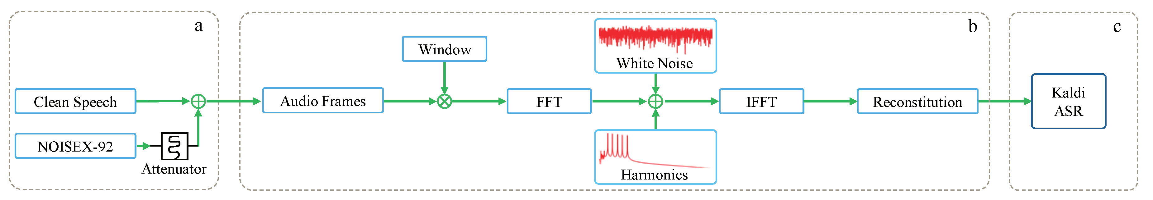
The block diagram of the verification experiment is illustrated in
Figure 5. The experiment includes an utterance generation module, a simulated DUT and a Kaldi ASR system, which corresponding to the part ‘a’, ‘b’ and ‘c’ in
Figure 5 respectively. The utterance generation module attenuates the white noise, babble noise and factory1 noise from the NOISEX-92 noise library by an attenuator according to the specified SNR, and then superimposes them on the clean speech, respectively [
40]. The clean speeches are 10 short (each is about 10 s, all are 16 kHz sampling frequency and 16-bit sampling resolution) segments from a male. The simulated DUT distorts the input speeches according to the corresponding frequency response. For clarity of contrast, the simulated DUT ensures that the DUTs have harmonic distortions of the same relative magnitude at any non-zero input signal frequency. The phases of distorted spectral components are the same as the fundamental spectral components. Each output frequency of the simulated DUT is equal to the summation of the input signal and the distorted spectral components at this frequency. The ASR system consists of an open-source ASR toolkit Kaldi [
41] and a Mandarin TDNN chain model CVTE trained on commercial data.
4.1. Compare DUTs with the Same Existing Indexes
Figure 6 are the averaged spectrum of two DUTs, which have exactly the same SNR, THD, and SINAD indexes. The difference is the harmonic power distribution. Although DUT3 seems to have a clearer spectrum than DUT4, but there is a much higher second-order harmonic around the fundamental signal. Thus, it is difficult to distinguish the performance difference from the same existing indexes.
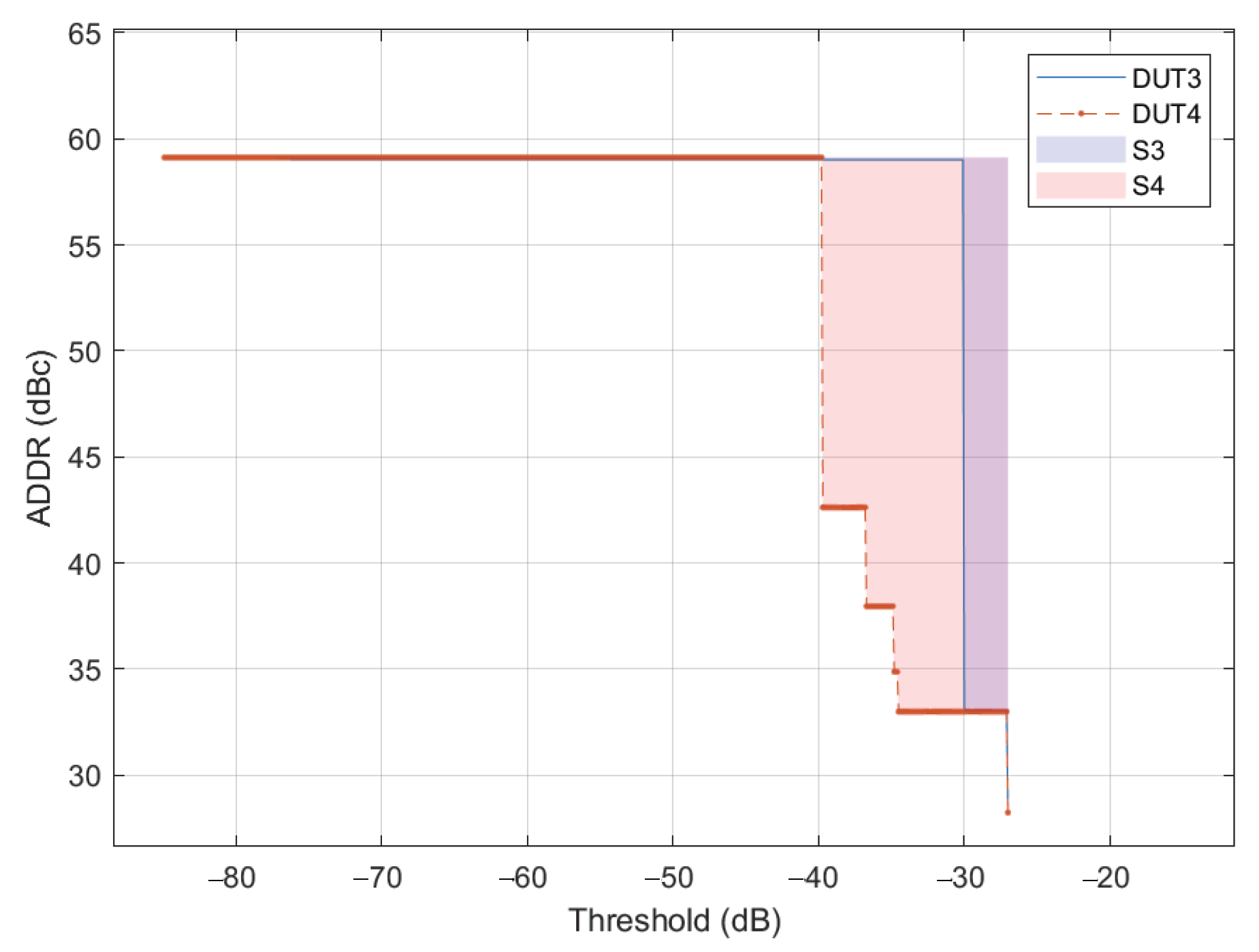
The ADDR plots corresponding to the above-mentioned DUT3 and DUT4 are shown in
Figure 7. The SNR and SINAD index of these DUTs are the same, which makes the ADDR plots have the same start and end positions. However, it is obvious that the middle parts of these ADDR plots are not the same, where the ADDR plot of DUT3 is higher than that of DUT4. This difference of the middle part results in the area of the specified region of DUT4 is smaller than that of DUT3. Based on the area comparison method and the judgement rules stated in Section II, Subsection B, the performance of DUT3 is better than DUT4 because the area ‘S3’ is smaller than ‘S4’.
Generally, under other conditions unchanged, the cleaner the speech through the ASR system is, the lower the WER is. Thus, the DUT with lower overall distortion will achieve a lower averaged WER. The averaged WERs of the test utterances distorted by the above-mentioned simulated DUT3 and DUT4 are shown in
Table 2, respectively.
The ‘ (%)’ column represents the WER differences of the latter DUT and the former DUT. In the ‘Match ?’ column, the symbol ‘√’ indicates that the comparison result of the ASR experiment is consistent with the comparison result of the ADDR plot, and the symbol ‘×’ indicates that the comparison result of the ASR and the comparison result of the ADDR are inconsistent, and the symbol ‘-’ indicates that the DUTs have the same WER. It can be seen that for different categories of noises, as the SNR setup gradually increases (larger attenuator setup), the WERs changes from a relatively poor level to relatively good level.
During the process, the averaged WER of the DUT3 and DUT4 is about 42.57%, and the WERs of DUT2 are on average 5.11% higher than that of DUT3. This difference accounts for 5.11/42.57 × 100% = 11.29%. Such a big difference is indistinguishable by existing indexes. However, a majority of ‘√’ symbols verify the conclusion of the ADDR plots.
In summary, the ADDR index can distinguish the performance difference of DUTs when they have the same SNR, SINAD, THD and SFDR indexes, which is an effective characteristic in real applications.
4.2. Performance Comparison of DUTs with Small difference of Different Existing Indexes
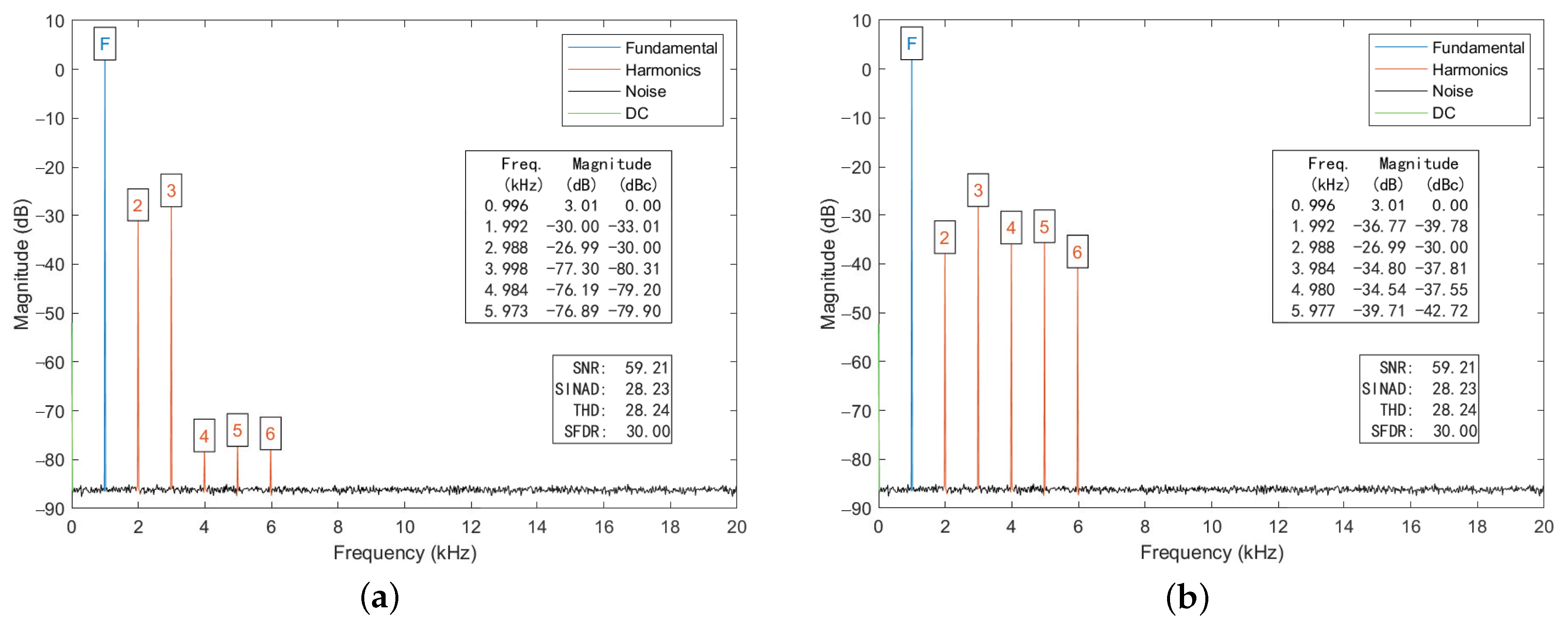
Figure 8a,b shows the averaged spectrum of DUTs, which have the advantage of different existing indexes. It can be seen that the SNR of DUT5 has an advantage of 2.05 dB than DUT6 while the SINAD and THD of DUT6 have advantages of 2.27 dB and 2.72 dB than DUT5 respectively. In this situation, it is relatively more difficult to distinguish the performance difference of the two DUTs according to the existing indexes.
The ADDR plots of the two DUTs are shown in
Figure 9. In the ADDR plot, the left and right sides of the intersection of two curves indicate that these two DUTs each have their own performance advantages. However, the area of the specified region of DUT5 is smaller than that of DUT6. Base on the judgement rules and the area comparison method in Section II, Subsection B, the performance of DUT5 is better than DUT6 because the area ‘S5’ is smaller than ‘S6’.
From
Table 3, it can be seen that the averaged WERs of these DUTs is about 27.24%, and the WERs of DUT2 are on average 0.88% higher than that of DUT5. This difference accounts for 0.88/27.24 × 100% = 3.23%. The difference is relatively much smaller, which means these DUTs have very close overall performances. There are three ‘×’ symbols in Table, which represent the contrary results with the conclusion of ADDR. But it should be noted that these three negative values are relatively smaller, and a positive averaged WER of 0.88% and relatively many ‘
√’ symbols verify the conclusion obtained by the ADDR plots to a certain extent.
In summary, the ADDR index can compare the performance of a DUT with a relatively high accuracy under some complicated comparison conditions. Therefore, it is an effective supplement to the existing indexes in some practical conditions.
5. Discussion
Comparing the proposed ADDR index with the SNR and SINAD indexes from the aspect of calculation method based on the spectrum, we can find that the existing indexes are equivalent to a fixed ADDR performance line, and the proposed ADDR plot is equivalent to connecting all the ADDR performance lines into a performance surface. Furthermore, the lifelike audio signals are generally nonstationary. For an audio DUT, the performance surface probably changes with the amplitude of the input signal. Therefore, a more practical and targeted comparison extends the proposed method from the two-dimensional area comparison to three-dimensional volume comparison, as is shown in
Figure 10.
The volume comparison is conducted on the ADDR performance body formed by the ADDR plot performance surface as a function of the amplitude of the input signal. Similarly, a smaller volume corresponding to better overall performance. At the same time, the ratio of each amplitude of the actual audio signal specified length in the time domain should be analyzed, and then the corresponding performance surface constituting the ADDR performance body should be weighted using this ratio.
Representing the proposed ADDR metric by a single number (quantifying the area in the ADDR-vs-threshold plot between the two reference lines and the plot-line) may be more useful. One possible idea is to set an absolute area that big enough to cover all the performance of practical audio systems on the output spectrum of the DUT, and then calculate the ratio of the area of the selected ADDR graph to that absolute area. The result will be between 0 to 1, and a value closer to 0 represents better performance.
The ADDR index may have a certain supplementary effect on the RF systems compared with the existing indexes. This is because the RF systems also have a certain working bandwidth, all the harmonic, spurious and noise components are the reasons of performance degradation. In addition to the existing indexes such as SFDR, ADDR may also comprehensively reflect the effects of distorted spectral components on RF systems. Similar to the uneven sensitivity to different distortions of human ears, the distorted components farther away from the fundamental wave generally have less influence, and this can be compensated with a weighting function on the spectrum before the calculation of ADDR plot.
6. Conclusions
This paper proposes a new audio system DR performance index called ADDR based on our new definition method. The ADDR index unifies the SNR (0 dBFS input) and the SINAD indexes while depicting extra performance details between the two indexes. Our first contribution is to propose an explicit definition of the ADDR index, which reduces the ambiguities of DR measurement. The second contribution is analyzing the critical factors that influence the accuracy of ADDR, and the corresponding optimal measurement conditions are given. Finally, we compare the ADDR index with some traditional indexes widely used in performance evaluation. A series of simulations verify the supplementary significance of our ADDR index relative to the existing indexes in the real applications because it comprehensively reflects the impact degree of all the distorted signals on DUT performance.


