PreNNsem: A Heterogeneous Ensemble Learning Framework for Vulnerability Detection in Software

Abstract

Automated vulnerability detection is one of the critical issues in the realm of software security. Existing solutions to this problem are mostly based on features that are defined by human experts and directly lead to missed potential vulnerability. Deep learning is an effective method for automating the extraction of vulnerability characteristics. Our paper proposes intelligent and automated vulnerability detection while using deep representation learning and heterogeneous ensemble learning. Firstly, we transform sample data from source code by removing segments that are unrelated to the vulnerability in order to reduce code analysis and improve detection efficiency in our experiments. Secondly, we represent the sample data as real vectors by pre-training on the corpus and maintaining its semantic information. Thirdly, the vectors are fed to a deep learning model to obtain the features of vulnerability. Lastly, we train a heterogeneous ensemble classifier. We analyze the effectiveness and resource consumption of different network models, pre-training methods, classifiers, and vulnerabilities separately in order to evaluate the detection method. We also compare our approach with some well-known vulnerability detection commercial tools and academic methods. The experimental results show that our proposed method provides improvements in false positive rate, false negative rate, precision, recall, and F1 score.

1. Introduction

Software vulnerabilities are one of the root causes of cybersecurity issues. Despite the improving software quality in academia and industry, new vulnerabilities have been exposed, causing huge losses. A large number of vulnerabilities were proven by Common Vulnerabilities and Exposures [1].

Vulnerability detection is an effective method for discovering software bugs. Overall, vulnerability detection methods can be categorized as static and dynamic methods. High coverage and low false positives are the advantages of static methods and dynamic methods, respectively. Many studies of source-code-based static analysis during the software development stage considered open-source tools [2,3,4], commercial tools [5,6,7], and academic research tools [8,9,10] to reduce dynamic runtime costs. Most of these tools are based on pattern matching. The pattern-based methods require experts to manually define vulnerability features for machine learning or rule matching. In summary, there are two significant drawbacks with the existing solutions: (1) relying on human experts and lacking automation; (2) the high false positive rate and low recall. Both are described below.

The existing solutions rely on human experts to define vulnerability features. It is difficult to guarantee the correctness and comprehensiveness of features because of complexity, even for experts. This is a highly subjective task, because the knowledge and experience of experts influence the results. It follows that there cannot be a unified standard for manually extracting features. Therefore, we must reduce or eliminate reliance on intense labor from human experts.

The existing solutions produce a high false positive rate and low recall. Most new tools detect all possible vulnerability patterns when matching the rules, regardless of context, structure, or semantics. As such, the detection results have low recall and a high false positive rate. Because of the fixed nature of rule detection, errors occur when detecting the same vulnerability across projects. Although machine learning has been applied to solve the above problems [11,12], the results are still unsatisfactory. These problems suggest that we must achieve a low false positive rate while maintaining a high recall rate.

For the two problems that are mentioned above, the featured engineer should be the core of the solution. Firstly, automated feature extraction will overcome the need for human labor. Secondly, precise vulnerability features will improve the precision of the result. As an automated feature tool, deep learning [13,14] was proposed for vulnerability detection. Applicable deep learning models can automatically and precisely learn various low- and high-level features. However, there are many deep-learning models, and one problem is selecting a model for achieving automation and a lower false positive rate.

In this paper, the proposed framework, which involves pre-training for vector representation, neural networks for automated feature extraction, and ensemble learning for classification (PreNNsem), focuses on improving the feature engineering of vulnerability detection. To validate PreNNsem, we applied different models of pre-training, neural networks, and ensemble learning. Word2vec continuous bag-of-words (CBOW), multiple structural convolutional neural networks (CNNs), and stacking classifiers were found to be the best combination by comparing classification results. In summary, we make four contributions:

• When compared with our prior work [15], we propose a framework for systematizing feature extraction to automatically detect vulnerabilities based on natural language processing. PreNNsem enables multiple kinds of deep neural networks to extract various kinds of vulnerability features.
• We transfer the standard language features in an extended corpus to the current model’s training and maintain its structural and semantic information through pre-training. We evaluate trainable and non-trainable pre-training methods in terms of detection capability and performance. It is essential to weigh the pros and cons of different pre-training methods for specific vulnerability detection tasks.
• We compare different neural network models to obtain features of vulnerability, providing a reference for future automated vulnerability detection. Improving the effectiveness of feature extraction, we compose a parallel and sequential architecture neural network.
• Our proposed method is more effective than the state-of-the-art methods. The experimental results show that PreNNsem is more useful than traditional static analysis tools and state-of-the-art vulnerability detection systems.

The remainder of this paper is structured, as follows: Section 2 reviews related work. Section 3 presents the PreNNsem framework. Section 4 describes our experimental evaluation of PreNNsem and comparison results and Section 5 discusses problems and concludes the paper.

2. Related Work

2.1. Prior Studies Related to Vulnerability Detection

From the degree of automation, previous vulnerability detection methods can be divided into three categories: (i) Manual methods: Many static vulnerability tools, such as Flawfinder [2], RATS [16], and Checkmarx [17], are based on vulnerability patterns, which are defined by human experts. Because pattern matching depends on the rule base, the false positives and/or false negatives are often high. (ii) Semi-automatic methods: Features are manually defined (code-churn, complexity, coverage, dependency, and organizational [18]; code complexity, information flow, functions, and invocations [19]; missing checks [20,21]; and, abstract syntax tree (AST) [22,23]) for traditional machine learning, such as k-nearest neighbor and random forest. MingJian Tang et al. [24] used artificial statistical characteristics to analyze vulnerability trends and dependencies with the Cupra model in multivariate time series. (iii) More automatic methods: Human experts do not need to define features. POSTER [25] presented a method for automatically learning high-level representations of functions. VulDeePecker [13] is a system showing the feasibility of using deep learning to detect vulnerabilities. Venkatraman S et al. [26] proposed a hybrid model by employing similarity mining and deep learning architectures for image analysis. Vasan D et al. [27] analyzed malware images while using a CNN in order to extract features and support vector machine (SVM) for multi-classification.

PreNNsem is an automated approach and an end-to-end vulnerability detection framework. When compared with the manual and the semi-automatic methods, our method abandons subjectivity. Therefore, the features obtained by our method are more persuasive and comprehensive. POSTER extracts features from the level of the function with a coarser granularity. PreNNsem extracts richer features directly from the word level. Compared with VulDeepecker, we have expanded the corpus in the word embedding layer to increase the precision of semantic expression. We used heterogeneous classifiers to improve the stability and accuracy of classification.

2.2. Prior Similar Studies

Pattern-based approach. Z. Li et al. [13] generated vectors from code gadgets using Word2vec, like us. They used Recurrent Neural Network (RNN)-based deep learning and SoftMax for learning classification. Liu S et al. [28] also used RNN for learning high-level representations of abstract syntax trees (ASTs). Duan X et al. [29] extracted semantic features while using code property graph (CPG), obtaining feature matrices by encoding the CPG. Finally, they used attention neural networks for learning classification. Lin G et al. [30] proposed a deep-learning-based framework with the capability of leveraging multiple heterogeneous vulnerability-relevant data sources for effectively learning latent vulnerable programming patterns.

Similarity-based approach. Vinayakumar R et al. [31] used a Siamese network to identify the similarity and deep learning architectures to classify the domain name. Zhao G et al. [32] encoded code control flow and data flow into a semantic matrix. They designed a new deep learning model that measures code functional similarity that is based on this representation. Xiao, Yang et al. [33] used a novel program slicing to extract vulnerability and patch signatures from the vulnerability function and its patched function at the syntactic and semantic levels. Subsequently, a target function was identified as potentially vulnerable if it matched the vulnerability signature but did not match the patch signature. Nair, Aravind et al. [34] examined the effectiveness of graph neural networks for estimating program similarity by analyzing the associated control flow graphs. In [35], they built a graph representation of programs called flow-augmented abstract syntax tree (FA-AST) and applied two different types of graph neural networks (GNNs) on FA-AST to measure the similarity of code pairs.

When compared with any pattern-based approach, the similarity-based approach is sufficient for detecting the same vulnerability in target programs. However, it cannot detect vulnerabilities in some code clones, including deletion, insertion, and rearrangement of statements. PreNNsem is categorized as a pattern-based approach to vulnerability detection. The existing pattern-based approaches have two problems: first, the extracted information’s granularity is rough; second, the data set used to learn vulnerability patterns is insufficient. In contrast to the studies reviewed above, PreNNsem has two advantages: first, it directly extracts features from code granularity in order to avoid the loss of information during feature abstraction. Second, by expanding the corpus, it can learn from common programming patterns and improve generalization capabilities.

3. Design of PreNNsem

3.1. Hypothesis

High-level programming languages, like C and JAVA, are designed for humans, and are closed to human expression. They have many similarities with natural language. For example, programming languages are probabilistic in definitions and context-dependent in grammar. Hence, we can borrow concepts from natural language processing (NLP) for vulnerability detection. We consider the concepts of code language and natural language as follows:

• Concepts: A slice of code—sentences, keywords, statements, characters, numbers—words.
  For natural language processing, we encoded each word as a vector and each sentence as a sequence of vectors. Therefore, distributed representations are based on an assumption; words that occur in the same context tend to have similar meanings [36].
  For vulnerability detection, we separated the code segment by tokenization and represented as a sequence of vectors. It has the same form as NLP. Therefore, we made assumptions for vulnerability detection.

Hypothesis 1.

In a programming language, a token’s context is its preceding and succeeding tokens. Tokens that occur in the same context tend to have similar semantics.

Hypothesis 2.

The same types of vulnerabilities have similar semantic characteristics. These characteristics can be learned from the context of vulnerabilities.

3.2. Overview of PreNNsem

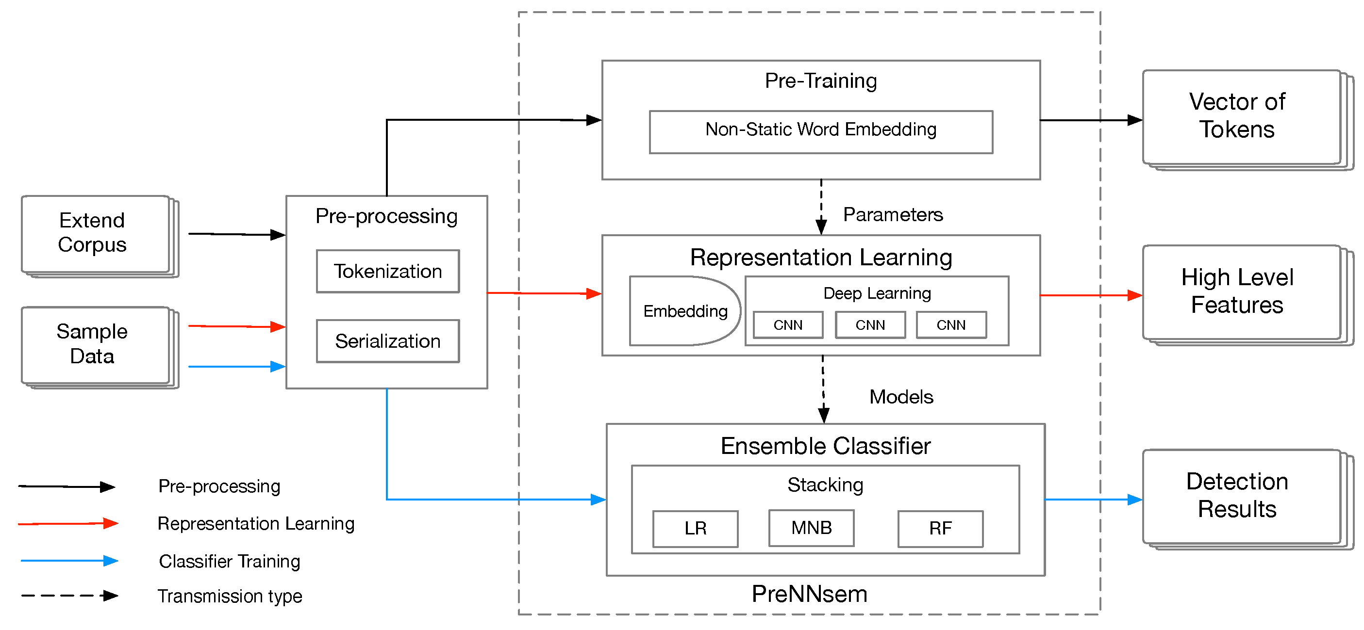
We aimed to automatically detect vulnerability with feature engineering, while using PreNNsem to achieve the goal. Figure 1 shows the process of our proposed framework, in which we take the sliced code as the input, and the output is whether the vulnerability is detected. In this paper, an extended corpus and sample data are transferred from C/C++ source code using security slice [13] and are represented as a sequence of numbers called “vectorize”. Subsequently, PreNNsem needs three steps that are related to each other. In this process, the intermediate data serve as the input to the next layer. In the first step, pre-training uses a vectorized extended corpus to generate distributed representation, and the output is a vector of tokens. The embedding layer takes the output as the initialization parameter. In the second step, the sample data pass through the embedding layer. The neural network and the SoftMax layer obtain high-level features. In the third step, supervised learning takes the feature as the input to determine whether the sample is vulnerable.

3.3. Source Code Pre-Processing

According to code lexical analysis, we remove some semantically irrelevant symbols (e.g., }{) in order to improve efficiency. We divided segment code into words by spaces and symbols (e.g., +−*/=). Deep learning models take vectors (arrays of numbers) as the input. When working with text, we had to develop a strategy to convert strings to numbers before feeding it to the model. Firstly, we indexed each word as a unique number. For example, we assigned 1 to “i”, 2 to “for”, 4 to “=”, 3 to “100”, and so on. Subsequently, we encoded the sentence “for i = 100” as a dense vector like [2, 1, 4, 3]. However, different sentences have different lengths. To unify data length for model input, we defined the max fixed-length as 400 according to sample data. There are two cases: if the sentence length is less than 400, zero will be padded; otherwise, the excess will be removed. Note that because pre-training requires a similar representation (Section 3.4) as embedding, extending the corpus only indexes the words in this step.

3.4. Word Embedding Pre-Training

According to Hypothesis 1, the same vulnerability pattern has similar semantics and structure in source code, and code representation is significant for pattern analysis. Word embeddings [37,38] are a type of word representation that allow words with similar meaning to have a similar representation. As such, a similar representation has the same vulnerability pattern. Vulnerability code and non-vulnerability code can be distinguished.

In this section, word embedding is divided into random, static, and non-static [39] embedding, according to the initialization method. Random embedding means all words are randomly initialized and then modified during training. Static embedding means word vectors are pre-trained from distribution representation and kept static and unchanged during training. Non-static embedding means pre-trained vectors from Word2vec are fine-tuned for each task and trained with a deep learning model. We used continuous bag-of-words (CBOW) to obtain densely distributed representation.

How does CBOW work? As shown in Figure 2, CBOW is a three-layer network. Firstly, we convert each word into a one-hot encoding form as the CBOW input. $x_{Ck}$ represents the vectors of surrounding words given a current word $x_t$, where C is the number of surrounding words and k is the number of vocabulary words. Every x is a matrix with a dimension of $k\times 1$. Secondly, we initialize a weight matrix $W_{k\times d}$ between the input layer and hidden layer. In $W_{k\times d}$, d is a word vector size. In the hidden layer, each x left multiples with W and then adds up to the average as the output $h_d$ of the hidden layer. $h_d$ is a matrix with a dimension of $d\times 1$

$$h_d=\frac{W^T·x_1+W^T·x_2+\dots +W^T·x_C}{C}$$

(1)

Next, we initialize a weight matrix $U_{d\times k}$ between the hidden layer and the output layer. In the output layer, h left multiples with U and then adds the $SoftMax$ activation function. y and x have the same dimensions, but each element of y represents each word’s corresponding probability distribution.

$$y=SoftMax(U^T·h)$$

(2)

The CBOW model is a method of learning. Finally, y is not the last result we want; the intermediate product W is the last word vector. In our proposed method, we define surrounding words windows $C=10$ and word vector size $d=200$. According to Figure 2, in CBOW, we want to predict the word of the target location. We use the location’s surrounding words as input and then obtain the probability distribution of vocabulary words. Finally, we select the word with the highest probability as the final result. In this process, the weight matrix W is constantly adjusted as the final word vector matrix.

3.5. Representation Learning

According to Hypothesis 2, common semantic characteristics can be learned from the context of vulnerabilities. Traditionally, the characteristics of manual definition are crucial to machine learning classification. They transform training data and then augment them with additional features to increase the efficacy of machine learning algorithms. However, with deep learning, we can start with raw data, as features will be automatically created by the neural network when it learns.

In this section, we choose CNN and Long Short-Term Memory (LSTM) as the base deep learning model. Figure 3 shows the selected deep learning model used in this study. Firstly, in order to better learn the structure and semantics of the data, we used transfer learning to build the embedding layer for neural networks. Secondly, we sequentially combined three concatenated CNNs and one CNN as a network model. Thirdly, we added a one-dimensional max-pooling layer and a dropout layer for dimension reduction.

What are the features learned by CNN? As shown in Figure 3, we represent a code segment of length n as:

$$S=[v_0,v_1,\dots ,v_n]$$

(3)

where $v_i$ is the ith word vector in the segment. A filter $w_h$ is used to extract new features combined by the following h words. h is the size of the filter $w_h$; $c_i^h$ represents the feature generated by combining the ith word and the h words following it.

$$c_i^h=f(w_h{v}_{i:i+h-1}+b),$$

(4)

where f is a non-linear function, b is a bias, and:

$$v_{i:i+h-1}=v_i\oplus v_{i+1}\oplus \dots \oplus v_{i+h-1},$$

(5)

where ⊕ is the concatenation operator. According to the filter size, there are four different types of filters, including size three, size four, size five, and size six filters. We considered a filter in order to generate a new feature. The larger the filter size, the richer the context of consideration. In our experiment, we applied multiple filters to multiple features. CNN is characterized by parallelism, and each filter is not related to each other, which improves the execution efficiency.

According to Figure 4, LSTM processes one code segment at a time, and the loop allows for information to be passed from one step of the network to the next. This chain-like nature reveals that the recurrent neural networks are intimately related to sequences. They are the genetic architecture of the neural network to use for such data.

In the application of extracting sequence features, RNN can obtain more comprehensive inter-sequence information than CNN. In theory, CNN can only consider consecutive words’ characteristics, and RNN can consider the entire sentence. However, in the experiment, the more information stored, the longer the processing time. Even if LSTM has chosen to forget some of the information, there is still the problem of prolonged time consumption for long sequences.

3.6. Heterogeneous Ensemble Learning

Recent experimental studies [40] showed that the classifier ensemble may improve the classification performance if we combine multiple diverse classifiers that disagree with each other. Neural network models are nonlinear and have a high variance, which can cause problems when preparing a final model for making predictions. A solution to the high variance of neural networks is to train multiple models and combine their predictions. Ensemble is a standard approach in applied machine learning to ensure that the most stable and best possible prediction is made. We replaced the simple SoftMax classifier with the stacking learning classifier to improve vulnerability classification.

According to [41], heterogeneous ensemble methods have emerged as robust, more reliable, and accurate, intelligent techniques for solving pattern recognition problems. They use different basic classifiers in order to generate several different hypotheses in the feature space and combine them to achieve the most accurate result possible.

How does the stacking framework work? Figure 5 shows the conception of the stacking ensemble. Stacking is used to combine multiple classifiers generated using different learning algorithms $L_1,\dots ,L_N$ on a training dataset S and a testing dataset $S^{\prime }$, which consist of samples $s_i=(x_i,y_i)$ ($x_i$: feature vectors, $y_i$: classifications). Define C as a classifier. Thus,

$$\left\{\begin{array}{cc}{C}_i=L_i\left(S\right),\hfill & \hfill i\in 1,\dots ,N\\ C_{meta}=L_{meta}\left(S^{\prime }\right)\hfill \end{array},\right.$$

(6)

where $C_i$ is the base classifiers and $C_{meta}$ is a meta classifier. In the first stage, we choose two base algorithm, $L_1=LogisticRegression$ and $L_2=MultinomialNaiveBayesian$. We divide training data into $K=10$ parts, one of which is the validation subset $S_d,d\in 1,\dots ,K$. We trained $C_i$ on S and evaluated while using 10-fold cross-validation. For the model trained in each step d, we complete predictions on the test set $Y^{\prime }$. $\forall i\in 1,\dots ,N,$ and $\forall d\in 1,\dots ,K.$

$$\left\{\begin{array}{cc}{C}_i^d=L_i(S-S_d)\hfill & \\ Y_i^d=C_i^d\left(S_d\right)\hfill & \\ P_i^d=C_i^d\left(S^{\prime }\right)\hfill & \end{array}\right.$$

(7)

Subsequently, each $Y_i^d$ is stacked into a feature $A_i$. Take the average of all $P_i$ to obtain feature $B_i$.

$$\left\{\begin{array}{cc}{A}_i=Y_i^1\uplus Y_i^2\uplus Y_i^3\uplus \dots \uplus Y_i^d\hfill & \\ B_i=average(P_i^1,P_i^2,P_i^3,\dots ,P_i^d)\hfill & \end{array}\right.$$

(8)

In the second stage, we concatenate $A_i$ to form a new training data A and concatenate $B_i$ to form new testing data B.

$$\left\{\begin{array}{cc}A=A_i⨁A_i⨁A_i⨁\dots ⨁A_i\hfill & \\ B=B_i⨁B_i⨁B_i⨁\dots ⨁B_i\hfill & \end{array}\right.$$

(9)

Finally, the meta-classifier is trained on A and predict the result of B.

$$\left\{\begin{array}{cc}{C}_{meta}=L_{meta}\left(A\right)\hfill & \\ Result=C_{meta}\left(B\right)\hfill & \end{array}\right.$$

(10)

3.7. Construct Framework

Now, we build a vulnerability detection framework and propose an implementation. Our proposed framework (PreNNsem) consists of distributed representation, deep learning, and machine learning. We chose an implemented solution, Word2vec CBOW, for distributed representation, multiple structural CNNs for deep learning, and heterogeneous ensemble classifier (stacking) for machine learning.

We tokenize the extended corpus in order to obtain word vectors for similar code representations. Sample data are indexed and sequenced as input to the deep learning model. Word vectors are used as a parameter of the embedding layer. The processed sample data are embedded with neural networks as the input to generate an automatic feature extraction model. Subsequently, features are trained by machine learning and predict whether the samples are vulnerable or not.

4. Experiments and Results

4.1. Evaluation Metrics

Let true positive (TP) denote the number of vulnerable samples detected correctly, false positive (FP) denote the number of normal samples detected incorrectly, false negative (FN) denote the number of vulnerable samples undetected, and true negative (TN) denotes the number of clean samples classified correctly. Running time and memory were considered for testing resource consumption.

We used five metrics to measure vulnerability detection results. The $FP$ rate ($FPR$) metric measures the ratio of falsely classified normal samples to all normal samples.

$$FalsePositiveRate\left(FPR\right)=FP/(FP+TN)$$

(11)

False negative rate ($FNR$) measures the ratio of vulnerable samples classified falsely to all vulnerable samples.

$$FalseNegativeRate\left(FNR\right)=FN/(FN+TP)$$

(12)

Precision measures the correctness of the detected vulnerabilities.

$$Precision\left(P\right)=TP/(TP+FP)$$

(13)

Recall represents the ability of a classifier to discover vulnerabilities from all vulnerable samples.

$$Recall\left(R\right)=TP/(TP+FN)$$

(14)

The $F1$ measure considers both precision and recall.

$$F1-Measure\left(F1\right)=2\ast P\ast R/(P+R)$$

(15)

The low $FPR$ and $FNR$, and high P, R, and $F1$ metrics indicated the excellent performance in the experimental results. Low resource consumption is also vital.

4.2. Experimental Setup

In terms of collection programs, the Software Assurance Reference Dataset (SARD) [42] serves as the standard dataset to test vulnerability detection tools with software security errors, and the National Vulnerability Database (NVD) [43] contains vulnerabilities in production software. In the SARD, each program case contains one or multiple common weakness enumeration Identifiers (CWE IDs). In the NVD, each vulnerability has a unique common vulnerabilities and exposures identifier (CVE ID) and a CWE ID to identify the vulnerability type. Therefore, we finally collected the programs with CWE IDs that contained vulnerabilities.

We chose two types of vulnerabilities as detection object: buffer overflow (CWE-119) and resource management error (CWE-399). We also collected some other C/C++ programs on NVD as an extended corpus for pre-training.

Table 1. Statistics on training data and pre-training data.

Datasets	Samples	Vulnerable	Not Vulnerable	Vocabulary
CWE-119	39,753	10,440	29,313	80,692
CWE-399	21,885	7285	14,600	37,499
Extended dataset	420,627	56,395	364,232	89,642

summarizes statistics on training data and pre-training data. The datasets were preliminarily processed by [13]. We collected data from the 10,440 programs related to buffer error vulnerabilities and 7285 programs related to resource management error vulnerabilities from the NVD; we also collected 420,627 programs as an extended corpus to improve code representation. The extended dataset focuses on 1591 open-source C/C++ programs from the NVD and 14,000 programs from the SARD. It includes 56,395 vulnerable samples and 364,232 samples that are not vulnerable.

Regarding training programs vs. target programs, we randomly chose 80% of the programs that were collected as training programs and 20% as target programs. This ratio is applied when dealing with one or both types of vulnerabilities. We also used 10-fold cross-validation over the training set to select the model and used the test set to test the obtained model.

For the deep learning model, we implemented the deep neural network in Python with Keras [44]. We ran experiments on a Google Colaboratory [45] with Nvidia K80, T4, P4, or P100 graphics processing unit (GPU). Genism [46] Word2vec was used to train the word embedding layer. Scikit-learn [47] provides KNeighborsClassifier, RandomForestClassifier, MultinomialNB, and LogisticRegression algorithm as classifiers. Every experiment monitored valid F1 as a condition of early stopping in 10 epochs.

Table 2. Tuned parameters for representation learning.

Parameter	Description
Input_dim	The size of sample vocabulary.
Output_dim	The dimensionality of vectors to which the tokens are converted (200).
Sequence_length	The length of each sample (400).
CNN units	There are 4 CNNs with128 filters each, and the sizes of the filters are 3, 4, 5, 6.
Batch_size	The number of samples that are propagated through the network (128).
Loss function	A function to calculate the loss between the predicted value and real value (binary_crossentropy).
Optimizer	The algorithm to optimize the neural network (Adam)
Monitor	The metric to be monitored for early stop (F1) and patience (10).

shows the parameters in the representation learning phase.

4.3. Comparison of Different Embedding Methods

We compared CBOW and Skip-gram to verify the effect of the embedding method. Different types of tokens were selected to test the methods. Then, their embedded results were lowered to a two-dimensional diagram, as shown in Figure 6. CBOW performed better. After embedding, semantically similar words are closer to each other in the diagram, which means that word embedding extracts token semantic information in the context code structure. CBOW is more accurate than the information extracted by Skip-gram.

4.4. Comparison of Different Neural Networks

We trained six neural network models on the CWE-119 dataset to evaluate the different neural network models for representation learning. Note that we only indexed and sequenced the dataset instead of vectorizing, so the training dataset is two-dimensional in this section. The models contained: (1) three sequential CNNs with128 filters each; (2) two long short-term memory (LSTM) layers, with a 128-dimensional output; (3) bidirectional long short-term memory (BiLSTM) with a 128-dimensional output; (4) combined CNN (128) and BiLSTM ($64\times 2$); (5) combined CNN, BiLSTM, and Attention; and, (6) sequentially combine three concatenated convolutional layers and one convolutional layer. To avoid the disappearance of gradients during RNN structural training, in networks that use LSTM, we use sigmoid as the last dense layer activation function, which is different from our previous papers [15].

Table 3. Comparison of different representation learning models. CNN, convolutional neural networks. convolutional; BiLSTM, bidirectional long short-term memory; FPR, false positive rate; FNR, false negative rate; P, precision; R, recall; F1, f1-score.

Models	FPR (%)	FNR (%)	P (%)	R (%)	F1 (%)
Sequential CNNs	7.2	80.8	48.0	19.2	27.4
Sequential LSTM	12.2	47.5	60.2	52.5	56.1
BiLSTM	10.6	51.5	61.4	48.5	54.2
CNN + BiLSTM	8.0	72.7	54.5	27.3	36.3
CNN + BiLSTM + Attention	8.6	67.5	57.0	32.5	41.4
Concatenated CNNs + CNN	7.4	76.2	52.9	23.8	32.8

shows the comparison results.

Within the margin of error, sequential CNNs and concatenated CNNs achieved the best FPR result. Sequential LSTM has balanced performance and achieved the best results in FNR, recall, and F1. It also has excellent precision. Of the CNNs, concatenated CNNs perform better. Therefore, we tested the embedding layer on sequential LSTM and concatenated CNNs.

4.5. Combination of Different Embedding Methods and Different Neural Networks

According to [39], we divided the pre-training into random, static, and non-static initialization, and then defined the vectors’ dimension as 200. Random initialization means that all words are randomly initialized and then modified during training. Static initialization means that all words are pre-trained from Word2vec to generate vectors and non-trainable in work. Non-static initialization means that pre-trained vectors are fine-tuned for each work. We used the CWE-119 dataset and tested different pre-training methods on the sequential LSTM and concatenated CNN models. For training the Word2vec embedding layer, we used CWE-119 as the corpus and SySeVR [48] data as the extended corpus. In this section, we count the memory and training time of the models to compare their resource consumption.

Table 4. Comparison of different embedding methods on different corpora. Memory, memory consumption; Time, time consumption.

Methods	Corpus	FPR (%)	FNR (%)	P (%)	R (%)	F1 (%)	Memory (MB)	Time (s/epoch)
CNN-random	-	3.4	12.3	90.1	87.7	88.9	1675.1	15.0
CNN-static	CWE-119	3.9	16.6	88.4	83.4	85.8	1671.0	9.9
CNN-non-static	CWE-119	2.5	10.7	92.6	89.3	90.9	1694.1	14.9
CNN-static	SySeVR	2.5	13.6	92.4	86.4	89.3	1670.9	10.1
CNN-non-static	SySeVR	2.6	9.7	92.3	90.2	91.2	1673.5	15.2
LSTM-random	-	2.1	12.9	93.5	87.1	90.2	1377.2	200.5
LSTM-static	CWE-119	2.3	13.4	92.8	86.6	89.6	1365.6	183.4
LSTM-non-static	CWE-119	1.9	9.8	94.1	90.2	92.1	1366.8	201.9
LSTM-static	SySeVR	1.6	10.5	95.1	89.5	92.2	1370.4	183.6
LSTM-non-static	SySeVR	2.3	10.7	93.0	89.3	91.1	1373.5	197.1

shows the comparison results.

As shown in Table 4, CNN excelled in terms of FNR and recall, and LSTM excelled for FPR and precision. However, the time consumption of LSTM was 18 times that of CNN. For both, we obtained the following conclusions. According to the corpus, the extended corpus has better metrics because the more words we trained, the more appropriate the obtained vector. According to the false rate (FPR + FNR), P, R, and F1, we found that trainable embedding is better than static embedding because the fine-tuning can be adjusted to each work. The memory of training is almost the same, because the input sample data and the embedding size were the same. Less time was required for static embedding because the increase in trainable parameters leads to increased training time.

In conclusion, when considering the results and efficiency, we chose non-static CNN with extending the corpus as our final deep learning model.

4.6. Comparison of Different Classification Algorithms

Through Section 4.4, we observed that concatenated CNNs are the appropriate deep learning model to extract features. In

Table 5. Comparison of different classification algorithms. ML, machine learning; KN, KNeighbors; LR, logistic regression; NB, MultinomialNB; GBDT, gradient boosting decision tree; RF, random forest.

Methods	Base Classifier	FPR (%)	FNR (%)	P (%)	R (%)	F1 (%)	Time (s)
Traditional ML	KN	6.5	22.3	80.6	77.7	79.1	0.7
Traditional ML	LR	5.6	27.1	81.9	72.9	77.1	0.7
CNNs + Traditional ML	KN	3.3	6.6	90.7	93.4	93.0	0.6
CNNs + Traditional ML	NB	5.6	6.1	85.4	93.9	89.5	0.1
CNNs + Traditional ML	LR	2.1	7.9	93.9	92.1	92.9	0.6
CNNs + Boosting	GBDT	1.6	9.1	95.5	90.7	93.0	48.8
CNNs + Bagging	RF	1.6	8.8	95.8	91.2	93.1	10.7
CNNs + Stacking	LR, NB, RF	1.5	8.0	95.4	91.9	93.6	13.7

, we directly use traditional machine learning after the word-embedding layer. In order to improve the classification results, we chose a different ensemble learning model [49] to substitute the simple activation sigmoid after CNNs. We chose boosting and bagging as our homogeneous ensemble model, including gradient boosting decision tree (GBDT) and random forest (RF). We used stacking for generating ensembles of heterogeneous classifiers, logistic regression (LR) and MultinomialNB (NB) as the base classifiers, and RF as the final classifier. For comparison with ensemble classifiers, we also chose traditional classifiers, including KNeighbors (KN), NB, and LR. Finally, Table 5 shows the comparison results.

Table 5 shows that the first two lines did not use representation learning to extract features, and the classification effect was poor. Machine learning with CNNs performed better than traditional machine learning. We concluded that word embedding can only extract the granular features of words. CNNs can obtain the features of code structure, not only word semantics. Therefore, multiple granularity features help to improve the performance of the classifier.

The results of the last three lines (CNN + Ensemble) were generally better than those of lines three to five. Although CNN + NB produced the best recall results (93.9%), its precision was worse, at 85.4%, resulting in an F1 score of only 89.5%, which represents comprehensive performance. Low precision leads to spending more effort and time on the wrong detection results. Therefore, ensemble learning can further improve vulnerability detection. Of the three ensemble learnings, the stacking that was used in this article yielded the best results because it combines multiple diverse algorithms to generate several different hypotheses in the feature space and achieves the most accurate result possible. Though time consumption is higher compared to traditional machine learning methods, we emphasize the detection results for vulnerability detection tasks. Therefore, the increased time consumption is within an acceptable range.

Above all, we selected the most appropriate implementation of PreNNsem through our experiments; it consists of non-static pre-training with an extended corpus, concatenated CNNs representation learning, and stacking classifier.

4.7. Ability to Detect Different Vulnerabilities

As shown in

Table 6. Comparison of different classification algorithms.

Vulnerability	Vulnerability Dataset	FPR (%)	FNR (%)	P (%)	R (%)	F1 (%)
Specific CWE ID	Buffer Overflow	1.5	8.0	95.4	91.9	93.6
	Resource Management Error	0.3	2.2	99.5	97.7	98.6
Multiple CWE IDs	Array Usage	2.6	7.9	92.3	92.1	92.2
	API Function Call	2.1	9.5	92.4	90.5	91.5
	Arithmetic Expression	1.4	5.2	92.7	94.8	93.8
	Hybrid Vulnerabilities	1.5	6.3	94.4	93.7	94.1

, the proposed method was applied to the six datasets. We tested our model on the buffer overflow CWE-119 dataset and resource management error CWE-339 dataset in order to evaluate our method’s detection ability for different types of vulnerabilities. To validate our approach’s generalization capabilities, we selected three different types of vulnerability datasets: Array Usage, API Function Call, and Arithmetic Expression. Each type of dataset contains multiple CWE vulnerabilities. Array Usage (87 CWE IDs) accommodates the vulnerabilities related to arrays (e.g., improper use of array element access, array address arithmetic, and address transfer as a function parameter). API Function Call (106 CWE IDs) accommodates the vulnerabilities related to library/API function calls. Arithmetic Expression (45 CWE IDs) contains the vulnerabilities that are related to improper arithmetic expressions (e.g., integer overflow). Finally, we combined the three to form a hybrid vulnerability dataset, Hybrid Vulnerabilities.

According to the results, we found that the method for detecting specific vulnerabilities performs well. Resource management error has the best result, F1 Score, at 98.6%. Our approach also performs well in detecting the same type of vulnerability. API Function Call has the lowest F1 score, but the result was still no less than 91.5%. The method performed better on hybrid vulnerability datasets than on the same vulnerability datasets, because having more data can improve the model’s indicators. In summary, our approach performs well on a variety of data sets.

4.8. Comparative Analysis

We compared our best experimental results with those of state-of-the-art methods in order to verify the performance of the proposed method. We chose open-source static analysis tool Flawfinder [2], commercial static analysis tool Checkmarx [17], vulnerable code clone detection tool VUDDY [50], and academic deep learning methods VulDeePecker [13], DeepSim [32], and VulSniper [29]. Our three reasons for selecting these were: (1) these tools represent the state-of-the-art static analyses for vulnerability detection; (2) they directly operate on the source code; and, (3) they were available to us. Flawfinder and Checkmarx represent manual methods based on static analysis. VUDDY is suitable for detecting vulnerabilities incurred by code cloning. VulDeePecker, DeepSim, and Vulsnipper use deep learning to analyze source code. All of the results in

Table 7. Comparison of experimental results obtained using the proposed method and those using state-of-the-art methods.

Method	FPR (%)	FNR (%)	P (%)	R (%)	F1 (%)
Flawfinder	46.3	69.0	23.7	40.5	29.9
Checkmarx	43.1	41.1	39.6	58.9	47.3
VUDDY	3.5	91.3	47.0	8.7	14.7
VulDeePecker	2.9	18.0	91.7	82.0	86.6
DeepSim	16.1	41.6	71.6	58.4	64.4
VulSniper	6.42	26.2	88.7	73.8	80.6
PreNNsem	1.5	8.0	95.4	91.9	93.6

are based on the CWE-119 dataset. The results of Checkmarx and VulDeePecker were obtained from [13]. The results of DeepSim and VulSniper were obtained from [29].

Our method outperformed the state-of-the-art methods. Because these traditional tools depend on the rule base, they incurred high FR (FPR and FNR) and lower precision, recall, and F1. VulDeePecker was found to be better than the other tools, with a precision of 91.7%. However, VulDeePecker’s recall rate was low, only 82.0%, because it does not expand the corpus during the word embedding phase. DeepSim and VulSnipper extract features from the intermediate code, which loses some of the information. Accordingly, both precision and recall do not work well. Our method automatically extracts vulnerability features directly from the slice source code and does not rely on the rule library. In the word embedding phase, we expand the corpus to obtain richer semantics. Therefore, we improved vulnerability detection capabilities. When compared to VulDeePecker, we improved FPR by 1.4%, FNR by 10%, pPrecision by 3.7%, recall by 9.9%, and F1 by 7%.

5. Conclusions

In this paper, according to existing detection methods, we analyzed vulnerability detection’s core problem, which is the lack of proper feature extraction. Firstly, we researched vulnerability detection methods related to deep learning. We then presented the PreNNsem framework to detect vulnerabilities by analyzing source code. We drew some insights that were based on the collected dataset, including explanations for word embedding, deep learning model, and classifier comparisons in vulnerability detection. We used six different vulnerability datasets to prove our method’s generalization ability. Finally, we compared the results that were obtained with our method with those of the state-of-art tools and academic methods to validate the improvement in vulnerability detection.

In terms of practicality, our summary is as follows: (i) our method performs well on various mixed vulnerability data sets. Our method can detect various vulnerabilities. (ii) Because we analyze the source code from the perspective of analyzing text, other high-level language source code vulnerabilities can also use our framework. (iii) Each part of PreNNsem also supports other methods, which proves the scalability of the framework.

However, our method has several limitations: (i) our method only focuses on the source program, and our framework can not be applied in executable programs. (ii) Our approach relies on VulDeePecker’s [13] code snipping, which will be proposed and integrated into our future framework. (iii) Although we chose several deep learning models, we need to evaluate other models. (iv) The sample length is padded if it is shorter than the fixed length and cut off if it is longer; future works need to investigate how to handle vectors’ varying lengths.