Calibrated Integral Equation Model for Bare Soil Moisture Retrieval of Synthetic Aperture Radar: A Case Study in Linze County

Abstract

Soil moisture plays a significant role in surface energy balance and material exchange. Synthetic aperture radar (SAR) provides a promising data source to monitor soil moisture. However, soil surface roughness is a key difficulty in bare soil moisture retrieval. To reduce the measurement error of the correlation length and improve the inversion accuracy, we used the surface roughness (Hrms, root mean surface height) and empirical correlation length lopt as proposed by Baghdadi to introduce analytical equations of the backscattering coefficient using the calibrated integral equation model (CIEM). This empirical model was developed based on analytical equations to invert soil moisture for Hrms between 0.5 and 4 cm. Experimental results demonstrated that when the incidence angle varied from 33.5° to 26.3°, R² of the retrieved and measured soil moisture decreased from 0.67 to 0.57, and RMSE increased from 2.53% to 5.4%. Similarly, when the incidence angle varied from 33.5° to 26.3°, R² of the retrieved and measured Hrms decreased from 0.64 to 0.51, and RMSE increased from 0.33 to 0.4 cm. Therefore, it is feasible to use the empirical model to invert soil moisture and surface roughness for bare soils. In the inversion of the soil moisture and Hrms, using Hrms and the empirical correlation length lopt as the roughness parameters in the simulations is sufficient. The empirical model has favorable validity when the incidence angle is set to 33.5° and 26.3° at the C-band.

1. Introduction

Soil moisture is a crucial state variable in the fields of hydrology, climatology, ecology, and agriculture [1,2,3,4]. With the development of remote sensing (RS) technology, large-scale monitoring of soil moisture has become a reality without expensive in situ monitoring networks. As an active microwave that can monitor soil moisture at a spatial resolution of meters to tens of meters under almost all weather conditions, synthetic aperture radar (SAR) is a promising data source to monitor soil moisture with relatively high prediction accuracy [5,6]. In recent years, as SAR satellite sensors develope from the earlier Seasat, ERS-1/2, JERS-1, RADARSAT-1 and other single-polarization space-borne sensors to the more recent ENVISAT/ASAR, SIR-C/X-SAR, ALOS/PALSAR, Sentinel-1, RADARSAT-2, TerraSAR-X, Cosmo-Skymed, GF-3, ALOS-2 multiband, and multipolarization satellite sensors, SAR has been widely used for soil moisture inversion [7,8,9,10,11].

According to the land cover class, the methods of soil moisture inversion using SAR data can be classified into two types: methods applied to bare soils [9,10,11] and methods for soils covered by vegetation [12,13,14,15,16,17]. For soil moisture inversion of soils with vegetation coverage, the key question is how to eliminate the effect of vegetation coverage on the backscattering coefficient. MIMICS and water-cloud models are currently used to describe the backscattering. Because of the complexity of the MIMICS model, the use of the water-cloud model became common [18,19]. El Hajj [20] developed an inversion approach to estimate surface soil moisture using sentinel-1/2 data based on the calibration of the water-cloud model. For soil moisture inversion of bare soil, the main problem is how to handle the soil surface roughness. Unsuccessful roughness parameterization has become the main source of error that affects the accuracy of soil moisture inversion. Currently, there are four conventional methods to parameterize the surface roughness [21]. The first method is change-detection analysis under the assumption of constant roughness. Rahman et al. [22] offered a solution strategy to estimate soil moisture using multiangle radar images without ancillary data. The second method is calibrating soil roughness parameters. Baghdadi et al. (2002) developed a calibrated integral equation model (CIEM), which used the empirical correlation length lopt to replace the correlation length l [23]. The third method is combining the semiempirical relations between the correlation length and root mean square height (Hrms). Zribi et al. (2014) proposed a new description of soil surface roughness for soil moisture [24]. The fourth method is using prior knowledge of the roughness state. Satalino et al. (2002) used prior information on the surface roughness of a given area to invert soil moisture [25]. There are other alternative approaches to the roughness problem, such as multiscale processes [26,27], two-dimensional surface roughness characterization [28,29], and polarization decomposition data usage [30,31]. There are also radar backscatter models that can correctly model the radar signal for a wide range of soil parameters in bare surface soil [32], which can be physical, semiempirical, or empirical. The most popular physical models are the integral equation model (IEM) [33], an IEM calibrated by Baghdadi, which is called the calibrated integral equation model (CIEM) in this paper [23,34,35,36,37,38], and the advanced integral equation model (AIEM) [39].

This paper intensively exploits the surface roughness by combining the change-detection analysis under the assumption of constant roughness and the calibrating soil roughness parameters. The approach attempts to use the backscattering of VV and VH polarizations and CIEM to invert soil moisture and surface roughness in bare soil. The surface roughness parameter can often be expressed as Hrms and the correlation length l. Fung has suggested that it is a difficult task to separately estimate the effects of Hrms and correlation length l on the backscattering behavior of rough surfaces [33]. Furthermore, Zbiri has indicated that when IEM/AIEM is used to simulate the backscattering characteristics, using only Hrms as a roughness parameter in the simulations is not sufficient to derive correct results because the effect of correlation length l on the backscattering coefficient is neglected [40]. In addition, Rahman et al. (2008) suggested that conducting field measurement of roughness may become impractical and expensive when large areas must be covered [22]. Therefore, many researchers [40,41,42,43] introduced a roughness parameter Zs (which is equal to Hrms²/l) expressed as the surface roughness to invert soil moisture. However, roughness parameter Zs adopted correlation length l in their studies. One study showed that the measurement error of correlation length l was much larger than that of Hrms in the roughness measurement of the fieldwork [35]. Therefore, how to reduce the error of the correlation length when the soil surface roughness is parameterized has become the major question to answer.

In this paper, the surface roughness defined by Hrms and the empirical correlation length lopt as proposed by Baghdadi were used to introduce analytical equations of backscattering coefficient using the CIEM. When the backscatter database was built to propose analytical equations of the backscattering coefficient, many researchers mostly used the IEM and AIEM, whereas CIEM was rarely used [40,41,44,45]. To compare the findings concerning the surface roughness parameterization and model, the related studies were summarized in

Table 1. Summary of the approaches in related papers.

Authors	Data Source	Model Used	Surface Roughness Parameterization
Zribi (2003) [40]	SIRC/X-SAR, ERASME, RADARSAT	IEM	Zs = s2/l
Yu (2010) [46]	ASAR	AIEM	Zs = s3/l2
Huang (2014) [47]	ENVISAT-ASAR	CIEM	Zs = s2/lopt
Tao (2017) [41]	ALOS/PALSAR, RADARSAT-2	IEM	Zs = s2.33/l1.33
Chen (2017) [48]	ASAR	AIEM	Zs = s3 + bs2l + cs2 + dsl + es + fl
Kong (2018) [45]	Radarsat-2	AIEM	Zs = s3/l
Yang (2019) [44]	RADARSAT-2	AIEM	Zs = s3/l2
Guo (2019) [49]	Sentinel-1	AIEM	Zs = $\surd 3$s/l
This Study	ASAR	CIEM	S,lopt

.

The paper developed an empirical model through numerical simulation and regression analysis based on CIEM. First, we discussed the effects of surface roughness defined by Hrms, empirical correlation length lopt and soil moisture mv on the backscattering coefficient simulations. Then, the relationship of the backscattering coefficient, Hrms, and soil moisture was established. In building the soil moisture inversion model, the combined roughness parameter was not used; only Hrms and the empirical correlation length lopt were used. Finally, this empirical model was developed based on the analytical equations to invert the soil moisture and surface roughness. The experimental results show that using Hrms and the empirical correlation length lopt as the roughness parameters in the simulations is sufficient for the inversion.

2. Study Area and Data

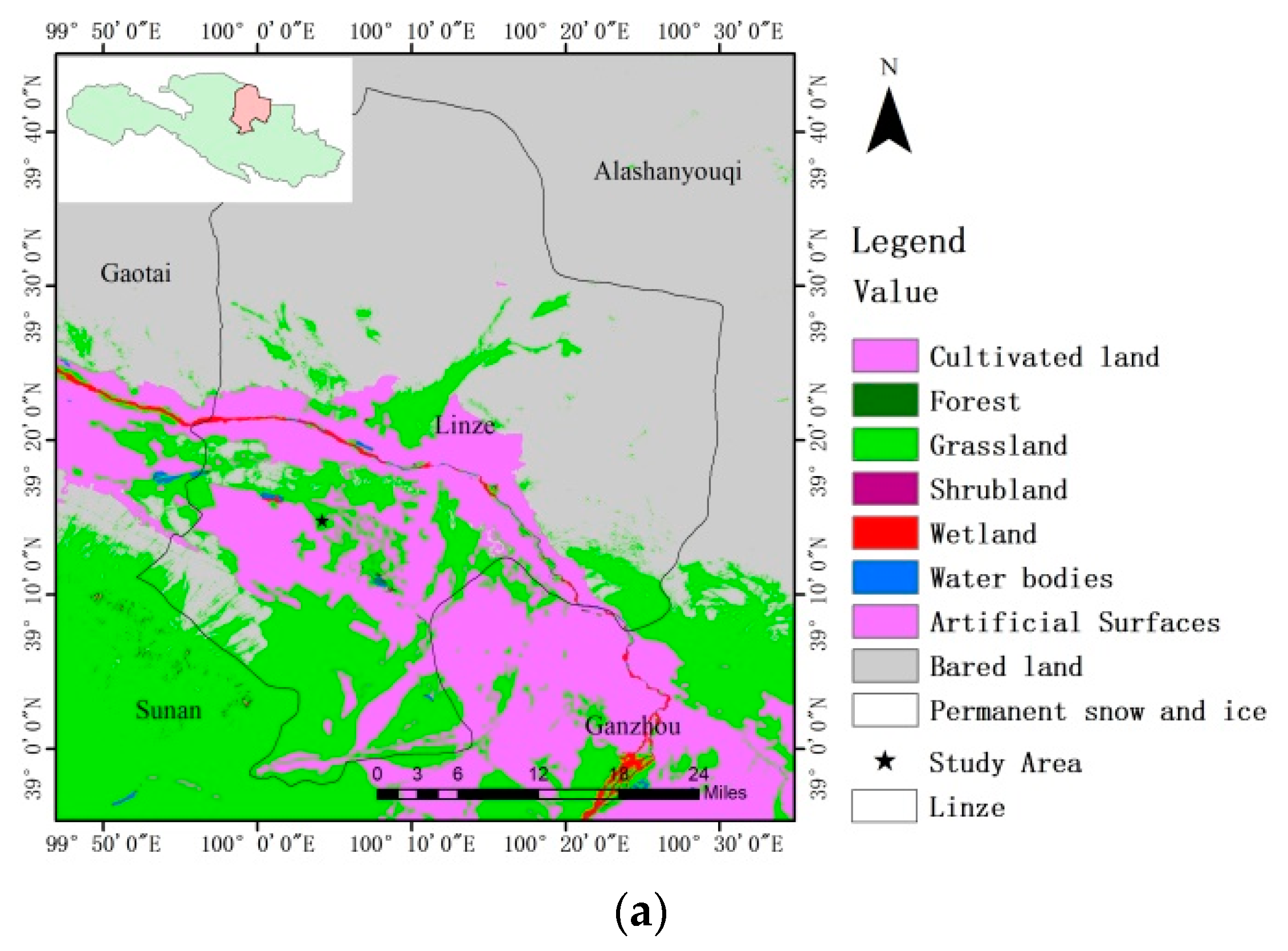
2.1. Study Area

In Figure 1, the study area is located in Linze County in Zhangye, Gansu province, China. The central position is 39.250 43° N, 100.005 871° E, and the altitude is 1385 m. The land cover map is obtained from GLC30 [50].

The region is in a temperate drought desert climate zone in the middle reach of Heihe River Basin with a flat terrain, which belongs to the lower plain part of the corridor. The average annual rainfall is 121.5 mm with an annual potential evaporation exceeding 2340 mm. The dry index is 15.9. The average temperature and annual sunshine hours are 7.1 °C and 3045 h, respectively. The ground features are mainly bare land and farmland with a small amount of sparse sedge. There is approximately 16.7% sandy soil, 74.8% sand, and 8.5% clay in the sand texture [46].

2.2. Satellite Data and Preprocessing

The Envisat ASAR satellite was equipped with a C-band SAR (5.405 GHz) with multipolarization, 7 observation angles and 5 operating modes. In the paper, ASAR data were used, whose operating mode was alternation polarization with two types of polarizations (VV and VH) and high space resolution (12.5 × 12.5 m per pixel). The ASAR data were provided on 11 July 2008 and 24 May 2008.

The satellite data were preprocessed with European Space Agency SNAP software. Radiometric calibration was applied, which can transform the digital number (DN) of each pixel of the original single-look complex product into the backscattering coefficient in decibels. An LEE filter with a 7 × 7 moving window was applied to weaken the effect of speckle noise. Then, range Doppler terrain correction was performed based on ACE30 DEM.

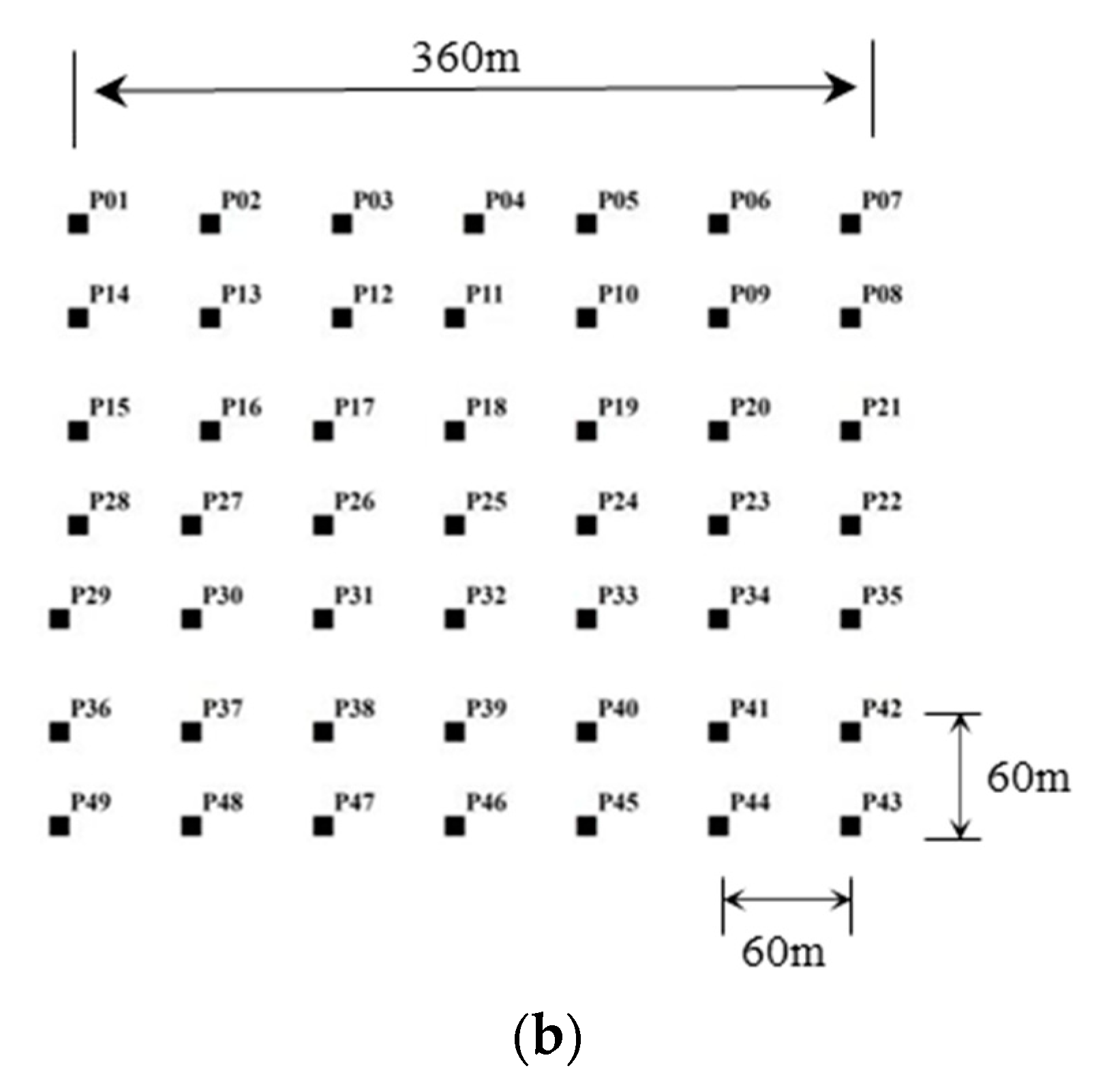
2.3. Ground Measurements Data and Analysis

Field measurement data were obtained from Watershed Allied Telemetry Experimental Research, including the surface soil moisture and surface roughness parameters [51,52,53]. The field measurements were taken while the satellite data were acquired. During this period, no precipitation or obvious temperature changes occurred in the experimental area.

The size of the study area is 0.36 × 0.36 km, and there are 49 sample points in this region. The soil samples were collected from the upper 0–5 cm soil layer. Most field measurements of soil moisture were made within ±2 h of the ASAR overpasses. The soil texture was analyzed by soil samples.

The soil moisture content of each sample point was measured by gravimetry. Firstly, the samples were obtained by a cutting-ring method, and the total weight of the soil was obtained using scales and expressed as G_wet. Secondly, the soils were dried, and the weight was expressed as G_dry. Thirdly, the volume of the cutting ring was provided, which was 50 cm³ and expressed as V_soil. Finally, the measured soil volume water content was calculated by the formula m_v = (G_wet − G_dry)/V_soil. The soil moisture in the field measurements was 13.5–50.7%.

The surface roughness data were measured using needle profilometers. which were 1 m long, and a digital camera. There were 101 needles with a 1-cm sampling interval between needles in the needle profilometers. At each sampling site, two field photographs were taken: along a north–south direction and along an east–west direction. Two roughness profiles were established for each sampling point. Standard deviations of Hrms and correlation length l were calculated using the mean of the autocorrelation function based on these measurements. The Hrms in the field measurements was 0.68–4.08 cm with an average of 1.4 cm, and the correlation length was 53–69 cm. The soil temperature was obtained by a needle thermometer, and it was observed twice at each sampling point. Detailed data are shown in

Table 2. ASAR images and simultaneous ground-based measurement data.

Satellite Data Description
Satellite Data	Polarization	Band	Acquisition Date	Incidence Angle (°)
ENVISAT/ASAR ENVISAT/ASAR	VV/VH VV/VH	C C	11 July 2008 24 May 2008	33.5° 26.3°
Ground Measurements Data
	Min	Max	Average	Observation Time
Soil moisture (%)	13.5	34.7	18.6	11 July 2008
Soil moisture (%)	17.6	50.7	24.7	24 May 2008
Hrms (cm)	0.68	4.08	1.4	7 June 2008
Correlation length (cm)	53	69	63.2	7 June 2008

.

3. Model Construction

3.1. Integral Equation Model and Calibrated Integral Equation Model

The IEM is the most commonly used physical model [54]. In the C-band, the validity domain of IEM [33] covers only a part of the range of roughness values commonly encountered for agricultural surfaces (k * Hrms ≤ 3 corresponds to Hrms ≤ 1.11 cm⁻¹ in C-band). The IEM describes the relationship between the backscattering coefficient with the characteristics of the sensor (incidence angle, polarization, and radar wavelength) and the soil properties (dielectric constant, Hrms, correlation length, and correlation function) over bare soils in agriculturally bare areas. It can be expressed as follows:

$$\begin{array}{l}{\sigma }_{pp}^0=\frac{k^2}{2}{\left|f_{pp}\right|}^2{e}^{-4Hrm{s}^2{k}^2{\cos }^2\theta }{\displaystyle \sum _{n=1}^{+\infty }\frac{{(4Hrm{s}^2{k}^2{\cos }^2\theta )}^n}{n!}}{W}^{(n)}(2k\sin \theta ,0)\\ +\frac{k^2}{2}\mathrm{Re}(f_{pp}^{*}{F}_{PP})e^{-3Hrm{s}^2{k}^2{\cos }^2\theta }{\displaystyle \sum _{n=1}^{+\infty }\frac{{(4Hrm{s}^2{\cos }^2\theta )}^n}{n!}}{W}^{(n)}(2k\sin \theta ,0)\\ +\frac{k^2}{8}{\left|F_{pp}\right|}^2{e}^{-2Hrm{s}^2{k}^2{\cos }^2\theta }{\displaystyle \sum _{n=1}^{+\infty }\frac{{(Hrm{s}^2{k}^2{\cos }^2\theta )}^n}{n!}}{W}^{(n)}(2k\sin \theta ,0)\end{array}$$

(1)

The CIEM is a semiempirical calibration model, which was proposed based on IEM by Baghdadi et al. [35,36]. The proposed CIEM adopts the empirical correlation length lopt and reduces the number of input soil parameters of the IEM from three to two (Hrms and mv only, instead of Hrms, l and mv). Correlation length l as the measured correlation length was replaced by a calibration parameter lopt included in the CIEM. Calibration parameter lopt (an empirical correlation length) is computed as a function of the Hrms, radar frequency, incidence angle, and polarization to obtain a better fit between CIEM simulations and radar observations.

The variable lopt in CIEM is not the input parameter but can be calculated in CIEM. Furthermore, it integrates the true correlation length and the imperfections of the IEM so that the simulated data using the CIEM can be consistent with radar measurement data.

For C-band SAR data, calibration parameter lopt can be expressed as follows [35,36]:

$$l_{opt\text{-}HH}(Hrms,\theta ,HH)=0.162+3.006{(\sin 1.23\theta )}^{-1.494}Hrms$$

(2)

$$l_{opt\text{-}HV}(Hrms,\theta ,HV)=0.9157+1.2289{(\sin 0.1543\theta )}^{-0.3139}Hrms$$

(3)

$$l_{opt\text{-}VV}(Hrms,\theta ,VV)=1.281+0.134{(\sin 0.19\theta )}^{-1.59}Hrms$$

(4)

where θ is in radians, and Hrms and lopt are in centimeters.

The CIEM has been successfully tested in many studies [11,55,56].

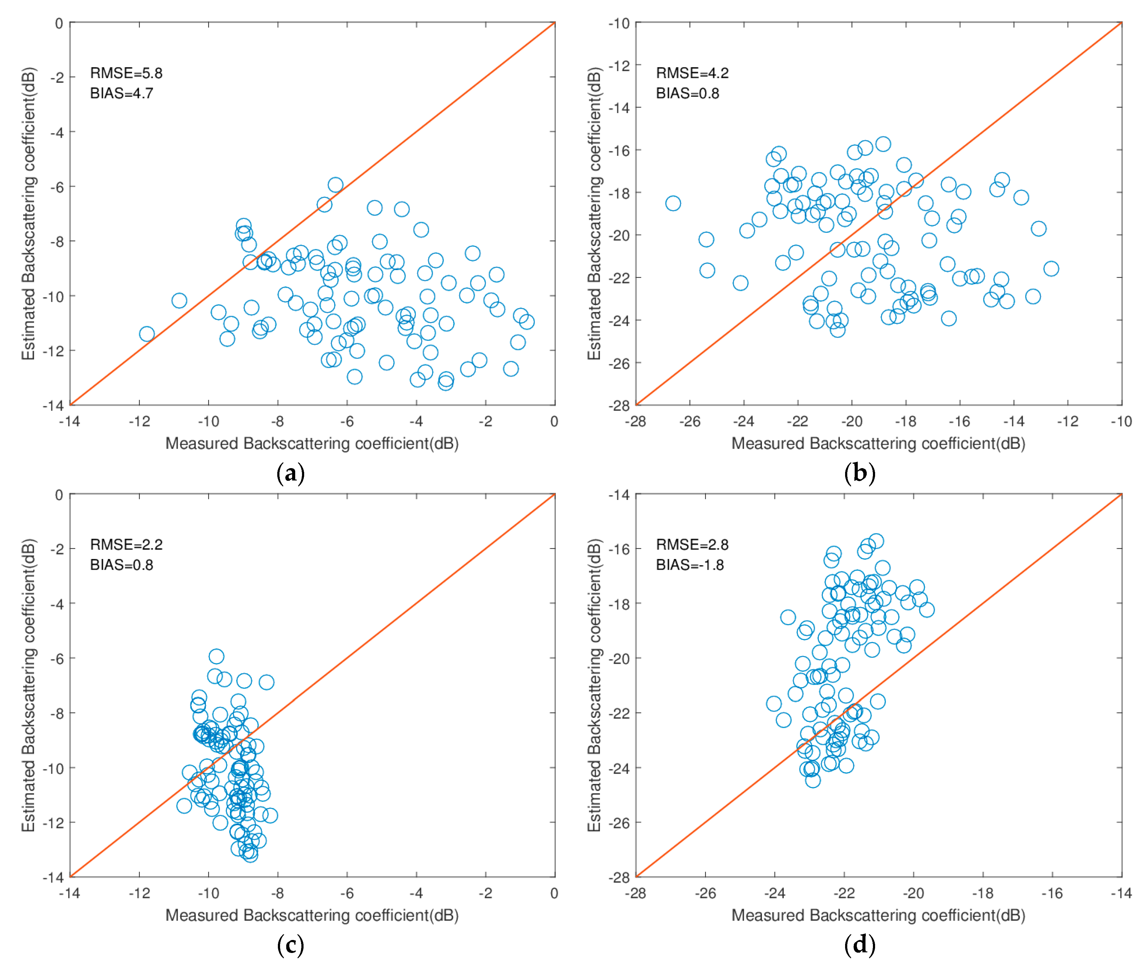
3.2. Comparison between CIEM and IEM

Both CIEM and IEM can provide backscattering coefficient values considering the characteristics of the sensor and target. In this section, the difference between IEM and CIEM of SAR for VV and VH polarizations in C-band was studied. In Figure 2, by using IEM, the biases are 4.7 dB in the VV polarization and 0.8 dB in the HV polarization. However, by using CIEM, the biases are 0.8 dB in the VV polarization and −1.8 dB in the HV polarization. In addition, the RMSE between the simulated and measured backscattering coefficient for VV polarization decreased from 5.8 dB to 2.2 dB after using CIEM, and the RMSE for HV polarization decreased from 4.2 to 2.8 dB. The results show that the CIEM performs better than the IEM, as observed by Baghdadi et al. [35,36]. Therefore, only CIEM was used to simulate the backscattering characteristics in this section.

3.3. Analysis of Simulated Backscattering Coefficient as Functions of Roughness and Soil Moisture

Shi et al. [57] suggested that the backscattering coefficients of a bare soil surface could be presented as a product of two functions on a linear scale:

$${\sigma }_{pq}(\theta )=R_{pq}({\epsilon }_s,\theta )\cdot S{r}_{pq}(\theta ,kHrms,kl)$$

(5)

or on a logarithmic scale [58]:

$${\sigma }_{pq}(\mathrm{dB})=10\log [R_{pq}({\epsilon }_s,\theta )\cdot S{r}_{pq}(\theta ,kHrms,kl)]$$

(6)

One function is the dielectric function R_pq that reflects the soil moisture information; the other is the roughness function Sr_pq that describes the effect of the surface roughness at a different polarization. σ_pq is the backscattering coefficient, where subscripts q and p represent the polarization status. Meanwhile, R_pq and functions Sr_pq are independent of each other. Firstly, this paper discussed the effects of Hrms and the empirical correlation length lopt on the backscattering coefficient using CIEM simulations in this section. Secondly, the effect of soil moisture mv on the backscattering coefficient using CIEM simulations was analyzed. Finally, the soil moisture inversion model was built using Equation (5) or Equation (6) based on the description of the model, which was built in Section 3.3.1 and Section 3.3.2.

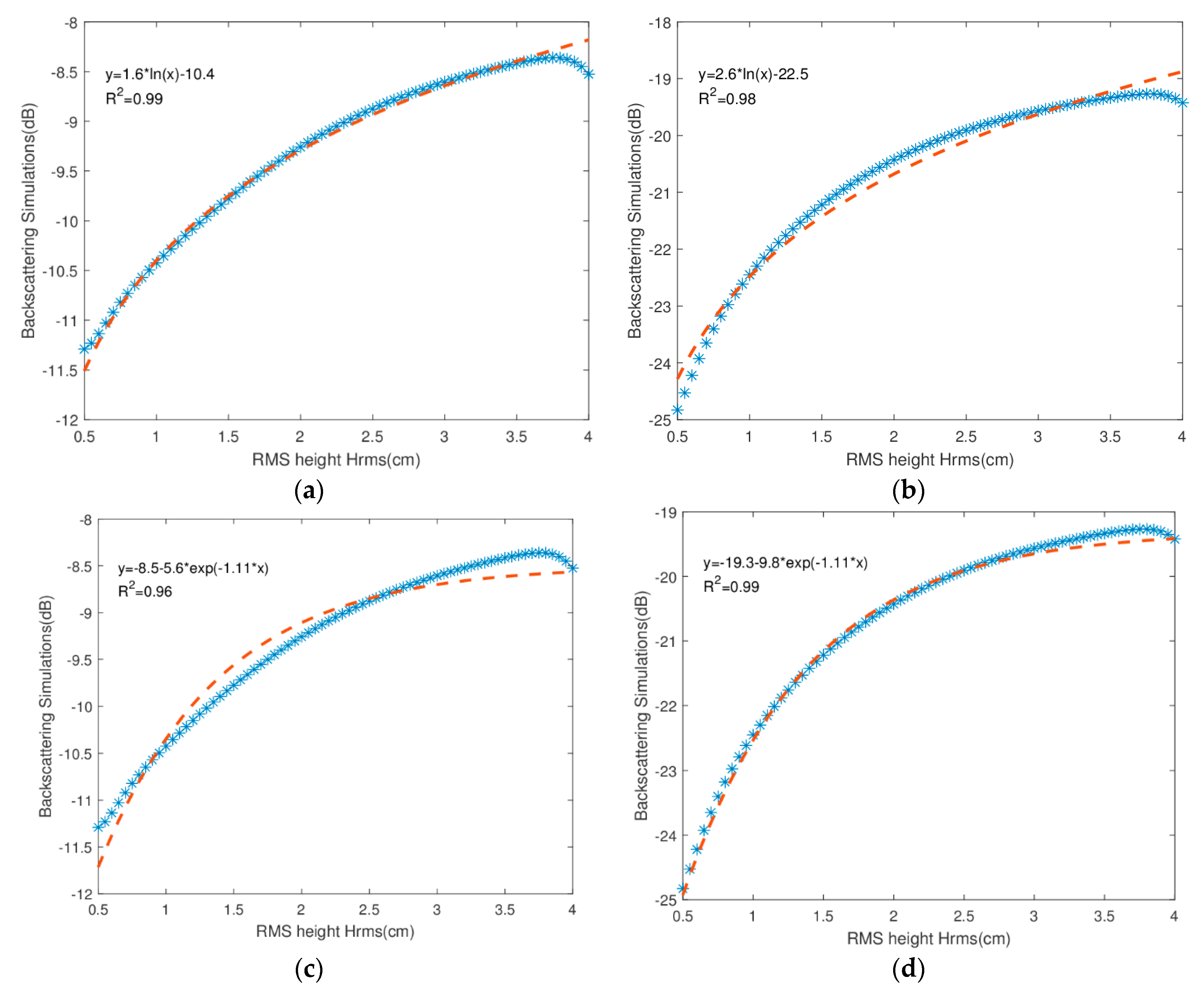
3.3.1. Effect of Hrms, Empirical Correlation Length lopt on the Backscattering Coefficient Using CIEM Simulations

As far as we know [24,40], two variables describe the surface roughness: Hrms and correlation length l. Studies have shown that the measurement error of correlation length l is much larger than that of Hrms in the contact measurement techniques on roughness because the shorter length profile and large sampling interval in field roughness measurements can result in substantially undervaluing the correlation length [59]. The error between the measured backscattering coefficients and the simulations by CIEM is mainly determined by the inaccuracy of correlation length l [35]. If the effect of the correlation length on the backscattering coefficient is neglected, it may cause large errors in the estimation of the backscattering coefficient. Therefore, the CIEM in this study did not use the measured correlation length l but used the empirical correlation length lopt instead. In building the model, variable incidence angle θ and wavelength λ can be considered constant at the C-band. Therefore, the correlation between backscattering coefficient and surface roughness is as follows:

$${\sigma }_{pq}(\theta )=S{r}_{pq}(\theta ,kHrms,k{l}_{opt})=S{r}_{pq}(\theta ,\frac{2\pi }{\lambda }Hrms,\frac{2\pi }{\lambda }{l}_{opt})=S{r}_{pq}(Hrms,l_{opt})$$

(7)

The calibration correlation length lopt in VV and HV polarizations can be expressed as Equations (3) and (4) in the CIEM. At the C-band, the incidence angle and frequency are known in VV and HV polarizations of the ENVISAT ASAR data, so variable incidence angle θ and frequency f can be considered constant. Equations (3) and (4) can be expressed as follows:

$$l_{opt}{}_{pq}=a+bHrms$$

(8)

where a and b are constants.

Therefore, combining Equations (5) and (7) yields the following expression:

$${\sigma }_{pq}(\theta )=S{r}_{pq}(Hrms,l_{opt})=S{r}_{pq}(Hrms,a+bHrms)=S{r}_{pq}(Hrms)$$

(9)

When the backscattering coefficient was simulated in CIEM, the volumetric soil moisture content was assumed to be 18.6%, which is the mean of the measured soil moisture at the incidence angle of 33.5°. Incidence angle θ is set to 33.5°, and frequency f is set to 5.405 GHz. The Hrms was supposed to be 0.5–4 cm using a step size of 0.05 cm, and the corresponding calibration correlation length lopt was calculated according to Equations (3) and (4). According to Baghdadi et al. (2006), the correlation function in the CIEM is Gaussian [35]. Figure 3 was obtained using statistical analysis.

This study found that R² of the logarithmic relationship in VV and VH polarizations both exceeded 0.98. Therefore, the logarithmic relationship was used to describe the roughness and backscattering coefficient, which can be expressed as follows:

$${\sigma }_{pq}\left(\mathrm{dB}\right)=A\ln (Hrms)+B$$

(10)

where A and B are the empirical coefficient, which can be calculated by statistical regression analysis.

This result of the study was validated by Baghdadi et al. (2002) [60].

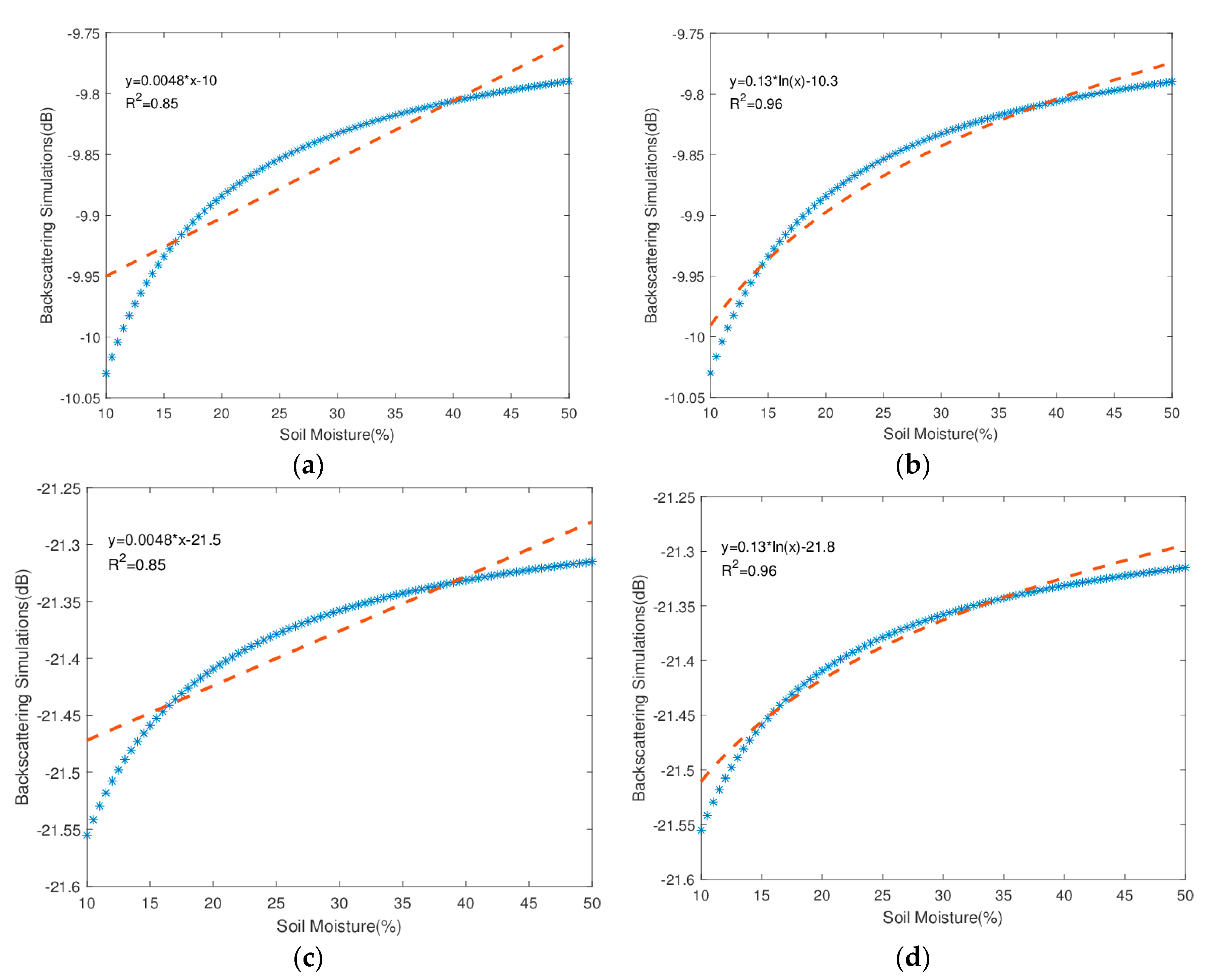
3.3.2. Effect of Soil Moisture mv on the Backscattering Coefficient Using CIEM Simulations

The relationship between soil moisture and backscattering coefficient was analyzed based on a CIEM simulated database under the following conditions: incidence angle θ is set to 33.5°; frequency f is set to 5.405 GHz; Hrms is 1.4 cm; corresponding empirical correlation length lopt can be calculated according to Equations (3) and (4); mv ∈ (10%, 50%) at intervals of 0.5%.

In Figure 4, when the surface roughness and radar configuration are fixed, there are different fitting relationships in VV and VH polarizations using two function expressions (linear and logarithmic). R² of the logarithmic relationship in VV and VH polarizations is 0.96, and the linear value is 0.85. The results show that the logarithmic relationship is better between soil moisture and backscattering coefficient, which can be expressed as follows:

$${\sigma }_{pq}\left(\mathrm{dB}\right)=C\ln (mv)+D$$

(11)

where C and D are the empirical coefficients, which can be calculated by a statistical regression analysis.

3.4. Soil Moisture Retrieval Model

Based on the above analysis, according to Equations (6), (10), and (11), the backscattering coefficient can be expressed as follows at a specific incidence angle and frequency:

$${\sigma }_{pq}(\mathrm{dB})=10\log \left[(A\ln (Hrms)+B)(C\ln (mv)+D)\right].$$

(12)

Therefore,

$${\sigma }_{pq}(\mathrm{dB})=10\log \left[a\ln (mv)+b\ln (Hrms)+c\ln (Hrms)\ln (mv)+d\right]$$

(13)

or

$$a\ln (mv)+b\ln (Hrms)+c\ln (Hrms)\ln (mv)+d{=10}^{\left({\sigma }_{pq}(\mathrm{dB})/10\right)}$$

(14)

where a, b, c, and d are regression coefficients that can be determined by least square methods, and p and q are the corresponding polarization mode.

4. Results and discussion

The retrieval model expresses the relationship between σ_pq, mv, and Hrms at a specific incidence angle and frequency. When the incidence angle is 25–55°, the logarithmic relationship of Equations (10) and (11) is better. Baghdadi et al. (2006) established that CIEM was calibrated in the C-band for a radar frequency of approximately 5.4 GHz. Therefore, the application condition of Equations (13) and (14) about the frequency is f = 5.4 GHz.

Then, the regression coefficients of the inversion model were discussed when the incidence angle changed. The database simulated by CIEM was built under the following conditions: frequency f was 5.4 GHz; Hrms was 0.5–4 cm with a step size of 0.1 cm; mv ∈ (10%, 50%) at intervals of 5%. Furthermore, the incidence angles of the empirical model were 25–55° with an interval of 5° to derive empirical coefficients at different incidence angles.

Table 3. Empirical coefficients at different incidence angles in VV polarization (Hrms ∈ (0.5, 4) cm).

θ (°)	a (θ)	b (θ)	c (θ)	d (θ)	R2
25	0.0032	0.0258	−9.592 × 10−5	0.104	0.57
26.3	0.0032	0.0286	1.973 × 10−4	0.1007	0.72
30	0.0031	0.0337	0.0008	0.0916	0.95
33.5	0.0030	0.0354	0.0011	0.0838	0.98
35	0.0030	0.0355	0.0012	0.0808	0.98
40	0.0029	0.0349	0.0014	0.0720	0.98
45	0.0028	0.0337	0.0015	0.0643	0.97
50	0.0028	0.0317	0.0017	0.0573	0.96
55	0.0029	0.0283	0.0018	0.0505	0.94

and

Table 4. Empirical coefficients at different incidence angles in VH polarization (Hrms ∈ (0.5, 4) cm).

θ (°)	a (θ)	b (θ)	c (θ)	d (θ)	R2
25	0.0001	0.0028	2.768 × 10−5	0.005	0.79
26.3	0.0002	0.0031	4.718 × 10−5	0.0051	0.86
30	0.0002	0.0037	9.666 × 10−5	0.005	0.97
33.5	0.0002	0.0041	0.0001	0.0053	0.99
35	0.0002	0.0042	0.0001	0.0053	0.99
40	0.0002	0.0045	0.0002	0.0053	0.99
45	0.0002	0.0046	0.0002	0.0051	0.99
50	0.0002	0.0045	0.0002	0.0048	0.98
55	0.0002	0.0041	0.0003	0.0043	0.98

show the values of empirical parameters a, b, c, and d at different incidence angles. In Table 3 and Table 4, when the Hrms was 0.5–4 cm and the incidence angle was 25°, R² of the empirical coefficient was only 0.57 and 0.79 in VV and VH polarizations, respectively; other values exceeded 0.94. However,

Table 5. Empirical coefficients at different incidence angles in VV polarization (Hrms ∈ (0.5, 2.5) cm).

θ (°)	a (θ)	b (θ)	c (θ)	d (θ)	R2
25	0.0037	0.0289	0.0010	0.1018	0.97
30	0.0032	0.0323	0.0011	0.0909	0.98
35	0.0030	0.0320	0.0012	0.0809	0.98
40	0.0029	0.0303	0.0012	0.0723	0.98
45	0.0028	0.0280	0.0012	0.0648	0.97
50	0.0028	0.0252	0.0012	0.0580	0.97
55	0.0029	0.0211	0.0012	0.0541	0.96

and

Table 6. Empirical coefficients at different incidence angles in VH polarization (Hrms ∈ (0.5, 2.5) cm).

θ (°)	a (θ)	b (θ)	c (θ)	d (θ)	R2
25	0.0002	0.0032	0.0001	0.0049	0.99
30	0.0002	0.0038	0.0001	0.0052	0.99
35	0.0002	0.0040	0.0002	0.0053	0.99
40	0.0002	0.0042	0.0002	0.0053	0.99
45	0.0002	0.0042	0.0002	0.0051	0.99
50	0.0002	0.0039	0.0002	0.0049	0.99
55	0.0002	0.0035	0.0002	0.0044	0.99

show that when the Hrms was 0.5–2.5 cm, R² of the empirical coefficient exceeded 0.96 in VV and VH polarizations. Therefore, the simulated values from the empirical model and CIEM compare fairly well at a specific incidence angle in VV and VH polarizations. When the maximum range of Hrms decreased from 4 to 2.5 cm and the soil surface was smooth, the empirical model had high accuracy.

In summary, the empirical model has good applicability at different incidence angles based on the above analysis. Therefore, the empirical model can be expressed as

$$a(\theta )\ln (mv)+b(\theta )\ln (Hrms)+c(\theta )\ln (Hrms)\ln (mv)+d(\theta ){=10}^{\left({\sigma }_{pq}(\mathrm{dB})/10\right)}$$

(15)

where 25° ≤ θ ≤ 55°.

5. Model Validation

To evaluate the performance of the retrieval model, the ENVSAT ASAR image was used to retrieve soil moisture in Linze County at an incidence angle of 33.5° and a frequency of 5.4 GHz. From Table 3 and Table 4, regression coefficients a, b, c, and d can be obtained as shown in Equations (16) and (17).

$$0.0030\ln (mv) + 0.0354\ln (Hrms) + 0.0011\ln (Hrms)\ln (mv) + 0.0838={10}^{({\sigma }_{\mathrm{vv}}(\mathrm{dB})/10)}$$

(16)

$$0.0002\ln (mv) + 0.0041\ln (Hrms) + 0.0001\ln (Hrms)\ln (mv) + 0.0053={10}^{({\sigma }_{\mathrm{vh}}(\mathrm{dB})/10)}$$

(17)

According to Equation (16), the following formula was obtained:

$$Hrms{=\mathrm{e}}^{\frac{{10}^{({\sigma }_{\mathrm{vv}}(\mathrm{dB})/10)}-0.0838-0.0030\ln (mv)}{0.0354+0.0011\ln (mv)}}$$

(18)

By substituting Equation (18) into Equation (17), the soil moisture mv can be calculated by MATLAB. Similarly, the Hrms can be calculated. Then, the approach of 3-fold cross validation can be used to validate the model by in situ data. Figure 5 and Figure 6 present the soil moisture and Hrms distribution map at the incidence angles of 33.5° and 26.3°, respectively. Figure 5 shows that when the incidence angle was set to 33.5°, the maximum value of soil moisture in the study area was 50%, and the maximum Hrms was 4 cm. When the incidence angle was set to 26.3°, the maximum value of soil moisture in the study area was also 50%, and the maximum Hrms was also 4 cm. In Figure 5, the brown color indicates higher soil moisture content and Hrms and the purple color indicates lower soil moisture content and Hrms. To evaluate the performance of the retrieval model, the retrieved and measured soil moisture values were compared, as shown in Figure 6. When the incidence angle varied from 33.5° to 26.3°, R² of the retrieved and measured soil moisture decreased from 0.67 to 0.57, and RMSE increased from 2.53% to 5.4%. In the same situation, when the incidence angle varied from 33.5° to 26.3°, R² of the retrieved and measured Hrms decreased from 0.64 to 0.51, and RMSE increased from 0.33 to 0.4 cm. The results show good consistency between simulated and measured data, but the inversion accuracy of soil moisture is higher than that of surface roughness. When the incidence angle varied from 33.5° to 26.3°, the inversion accuracy of soil moisture and surface roughness decreased. Therefore, it is feasible to invert soil moisture and surface roughness using the empirical model.

6. Conclusions

The paper developed an empirical model to invert both moisture content mv and surface roughness Hrms based on the database simulated by CIEM. In this study, the effects of the surface roughness Hrms, empirical correlation length lopt, and soil moisture mv on the backscattering coefficient using CIEM simulations were discussed. The relationship of backscattering coefficient σ, Hrms and soil moisture mv was used to invert the soil moisture and avoid the actual measurement error of correlation length l.

The main results of this work are summarized below:

(1) When the incidence angle varied from 33.5° to 26.3°, R² of the retrieved and measured soil moisture values decreased from 0.67 to 0.57, and RMSE increased from 2.53% to 5.4%. When the incidence angle varied from 33.5° to 26.3°, R² of the retrieved and measured Hrms decreased from 0.64 to 0.51, and RMSE increased from 0.33 to 0.4 cm. The results show that there is good consistency between simulated and measured data, but the inversion accuracy of soil moisture is higher than that of the surface roughness. Thus, using Hrms and the empirical correlation length lopt as the roughness parameters in the simulations is sufficient to invert the soil moisture and Hrms;

(2) The empirical model had favorable validity when the incidence angle was 33.5° and 26.3° at the C-band, but the accuracy was higher when the incidence angle was 33.5°;

(3) It is valid to invert soil moisture and Hrms based on CIEM, which uses an empirical correlation length lopt as proposed by Baghdadi, which avoids the actual measurement error of the correlation length and improves the inversion accuracy.

In summary, using Hrms and the calibration parameter lopt as the roughness parameters in CIEM is sufficient to invert the soil moisture and soil Hrms.

However, the computation of incidence angles in CIEM depends on the derivation and verification of the model because of the limited measured data. Therefore, a new incidence angle handling method will be studied. There is a dependence on the research area about the empirical model. In the future, we will attempt to develop a new calibrated advanced integral equation model to optimize the empirical model coefficients, so that the accuracy of soil moisture retrieval can be improved as much as possible.

References

1. Zhao, W.; Fang, X.; Daryanto, S.; Zhang, X.; Wang, Y.; Wenwu, Z.; Xuening, F.; Stefani, D.; Xiao, Z.; Yaping, W. Factors influencing soil moisture in the Loess Plateau, China: A review. Earth Environ. Sci. Trans. R. Soc. Edinb. 2018, 109, 501–509. [Google Scholar] [CrossRef]
2. Liu, C.-A.; Chen, Z.-X.; Shao, Y.; Chen, J.-S.; Hasi, T.; Pan, H.-Z. Research advances of SAR remote sensing for agriculture applications: A review. J. Integr. Agric. 2019, 18, 506–525. [Google Scholar] [CrossRef] [Green Version]
3. Lettenmaier, D.P.; Alsdorf, D.; Dozier, J.; Huffman, G.J.; Pan, M.; Wood, E.F. Inroads of remote sensing into hydrologic science during the WRR era. Water Resour. Res. 2015, 51, 7309–7342. [Google Scholar] [CrossRef]
4. Karthikeyan, L.; Pan, M.; Wanders, N.; Kumar, D.N.; Wood, E.F. Four decades of microwave satellite soil moisture observations: Part 1. A review of retrieval algorithms. Adv. Water Resour. 2017, 109, 106–120. [Google Scholar] [CrossRef]
5. Engman, E.T.; Chauhan, N. Status of microwave soil moisture measurements with remote sensing. Remote Sens. Environ. 1995, 51, 189–198. [Google Scholar] [CrossRef]
6. Wang, J.; Hsu, A.; Shi, J.; O’Neill, P.; Engman, E. A comparison of soil moisture retrieval models using SIR-C measurements over the little Washita River watershed. Remote Sens. Environ. 1997, 59, 308–320. [Google Scholar] [CrossRef]
7. Bousbih, S.; Zribi, M.; Lili-Chabaane, Z.; Baghdadi, N.; El Hajj, M.; Gao, Q.; Mougenot, B. Potential of Sentinel-1 Radar Data for the Assessment of Soil and Cereal Cover Parameters. Sensors 2017, 17, 2617. [Google Scholar] [CrossRef] [Green Version]
8. Santi, E.; Dabboor, M.; Pettinato, S.; Paloscia, S. Combining Machine Learning and Compact Polarimetry for Estimating Soil Moisture from C-Band SAR Data. Remote Sens. 2019, 11, 2451. [Google Scholar] [CrossRef] [Green Version]
9. Baghdadi, N.; El Hajj, M.; Choker, M.; Zribi, M.; Bazzi, H.; Vaudour, E.; Gilliot, J.-M.; Ebengo, D.M. Potential of Sentinel-1 Images for Estimating the Soil Roughness over Bare Agricultural Soils. Water 2018, 10, 131. [Google Scholar] [CrossRef] [Green Version]
10. Zhang, X.; Chen, B.; Fan, H.; Huang, J.; Zhao, H. The Potential Use of Multi-Band SAR Data for Soil Moisture Retrieval over Bare Agricultural Areas: Hebei, China. Remote Sens. 2015, 8, 7. [Google Scholar] [CrossRef] [Green Version]
11. Mirsoleimani, H.R.; Sahebi, M.R.; Baghdadi, N.; El Hajj, M. Bare Soil Surface Moisture Retrieval from Sentinel-1 SAR Data Based on the Calibrated IEM and Dubois Models Using Neural Networks. Sensors 2019, 19, 3209. [Google Scholar] [CrossRef] [Green Version]
12. Tao, L.; Wang, G.; Chen, W.; Li, J.; Cai, Q. Soil Moisture Retrieval from SAR and Optical Data Using a Combined Model. IEEE J. Sel. Topics Appl. Earth Obs. Remote Sens. 2019, 12, 637–647. [Google Scholar] [CrossRef]
13. Foucras, M.; Zribi, M.; Albergel, C.; Baghdadi, N.; Calvet, J.-C.; Pellarin, T. Estimating 500-m Resolution Soil Moisture Using Sentinel-1 and Optical Data Synergy. Water 2020, 12, 866. [Google Scholar] [CrossRef] [Green Version]
14. Bousbih, S.; Zribi, M.; El Hajj, M.; Baghdadi, N.; Lili-Chabaane, Z.; Gao, Q.; Fanise, P. Soil Moisture and Irrigation Mapping in A Semi-Arid Region, Based on the Synergetic Use of Sentinel-1 and Sentinel-2 Data. Remote Sens. 2018, 10, 1953. [Google Scholar] [CrossRef] [Green Version]
15. El Hajj, M.; Baghdadi, N.; Zribi, M.; Bazzi, H. Synergic Use of Sentinel-1 and Sentinel-2 Images for Operational Soil Moisture Mapping at High Spatial Resolution over Agricultural Areas. Remote Sens. 2017, 9, 1292. [Google Scholar] [CrossRef] [Green Version]
16. Gao, Q.; Zribi, M.; Escorihuela, M.J.; Baghdadi, N. Synergetic Use of Sentinel-1 and Sentinel-2 Data for Soil Moisture Mapping at 100 m Resolution. Sensors 2017, 17, 1966. [Google Scholar] [CrossRef] [Green Version]
17. Huang, S.; Ding, J.; Zou, J.; Liu, B.; Zhang, J.; Chen, W. Soil Moisture Retrival Based on Sentinel-1 Imagery under Sparse Vegetation Coverage. Sensors 2019, 19, 589. [Google Scholar] [CrossRef] [Green Version]
18. Zhang, L.; Lv, X.; Chen, Q.; Sun, G.-C.; Yao, J. Estimation of Surface Soil Moisture during Corn Growth Stage from SAR and Optical Data Using a Combined Scattering Model. Remote Sens. 2020, 12, 1844. [Google Scholar]
19. El Hajj, M.; Baghdadi, N.; Zribi, M.; Belaud, G.; Cheviron, B.; Courault, D.; Charron, F. Soil moisture retrieval over irrigated grassland using X-band SAR data. Remote Sens. Environ. 2016, 176, 202–218. [Google Scholar] [CrossRef] [Green Version]
20. Baghdadi, N.; El Hajj, M.; Zribi, M.; Bousbih, S. Calibration of the Water Cloud Model at C-Band for Winter Crop Fields and Grasslands. Remote Sens. 2017, 9, 969. [Google Scholar] [CrossRef] [Green Version]
21. Verhoest, N.E.C.; Lievens, H.; Wagner, W.; Álvarez-Mozos, J.; Moran, M.S.; Mattia, F. On the Soil Roughness Parameterization Problem in Soil Moisture Retrieval of Bare Surfaces from Synthetic Aperture Radar. Sensors 2008, 8, 4213–4248. [Google Scholar] [CrossRef] [Green Version]
22. Rahman, M.; Moran, M.; Thoma, D.; Bryant, R.; Collins, C.H.; Jackson, T.; Orr, B.; Tischler, M. Mapping surface roughness and soil moisture using multi-angle radar imagery without ancillary data. Remote Sens. Environ. 2008, 112, 391–402. [Google Scholar] [CrossRef]
23. Baghdadi, N.; King, C.; Chanzy, A.; Wigneron, J.P. An empirical calibration of the integral equation model based on SAR data, soil moisture and surface roughness measurement over bare soils. Int. J. Remote Sens. 2002, 23, 4325–4340. [Google Scholar] [CrossRef]
24. Zribi, M.; Gorrab, A.; Baghdadi, N. A new soil roughness parameter for the modelling of radar backscattering over bare soil. Remote Sens. Environ. 2014, 152, 62–73. [Google Scholar] [CrossRef] [Green Version]
25. Satalino, G.; Mattia, F.; Davidson, M.; Le Toan, T.; Pasquariello, G.; Borgeaud, M. On current limits of soil moisture retrieval from ERS-SAR data. IEEE Trans. Geosci. Remote Sens. 2002, 40, 2438–2447. [Google Scholar] [CrossRef]
26. Mattia, F.; Le Toan, T. Backscattering Properties of Multi-Scale Rough Surfaces. J. Electromagn. Waves Appl. 1999, 13, 419–526. [Google Scholar] [CrossRef]
27. Zribi, M.; Ciarletti, V.; Taconet, O. Validation of a Rough Surface Model Based on Fractional Brownian Geometry with SIRC and ERASME Radar Data over Orgeval. Remote Sens. Environ. 2000, 73, 65–72. [Google Scholar] [CrossRef]
28. Davenport, I.; Holden, N.; Pentreath, R. Derivation of soil surface properties from airborne laser altimetry. In Proceedings of the International Geoscience and Remote Sensing Symposium (IGARSS ’03), Toulouse, France, 21–25 July 2003; pp. 438–4391. [Google Scholar]
29. Davenport, I.; Holden, N.; Gurney, R. Characterizing errors in airborne laser altimetry data to extract soil roughness. IEEE Trans. Geosci. Remote Sens. 2004, 42, 2130–2141. [Google Scholar] [CrossRef]
30. Hajnsek, I.; Pottier, E.; Cloude, S. Inversion of surface parameters from polarimetric SAR. IEEE Trans. Geosci. Remote Sens. 2003, 41, 727–744. [Google Scholar] [CrossRef]
31. Schuler, D.; Lee, J.-S.; Kasilingam, D.; Nesti, G. Surface roughness and slope measurements using polarimetric SAR data. IEEE Trans. Geosci. Remote Sens. 2002, 40, 687–698. [Google Scholar] [CrossRef]
32. Baghdadi, N.; Choker, M.; Zribi, M.; El Hajj, M.; Paloscia, S.; Verhoest, N.E.C.; Lievens, H.; Frappart, F.; Mattia, F. A New Empirical Model for Radar Scattering from Bare Soil Surfaces. Remote Sens. 2016, 8, 14. [Google Scholar] [CrossRef] [Green Version]
33. Fung, A.; Li, Z.; Chen, K. Backscattering from a randomly rough dielectric surface. IEEE Trans. Geosci. Remote Sens. 1992, 30, 356–369. [Google Scholar] [CrossRef]
34. Baghdadi, N.; Gherboudj, I.; Zribi, M.; Sahebi, M.; King, C.; Bonn, F. Semi-empirical calibration of the IEM backscattering model using radar images and moisture and roughness field measurements. Int. J. Remote Sens. 2004, 25, 3593–3623. [Google Scholar] [CrossRef]
35. Baghdadi, N.; Holah, N.; Zribi, M. Calibration of the Integral Equation Model for SAR data in C-band and HH and VV polarizations. Int. J. Remote Sens. 2006, 27, 805–816. [Google Scholar] [CrossRef]
36. Baghdadi, N.; Chaaya, J.A.; Zribi, M. Semiempirical Calibration of the Integral Equation Model for SAR Data in C-Band and Cross Polarization Using Radar Images and Field Measurements. IEEE Geosci. Remote Sens. Lett. 2010, 8, 14–18. [Google Scholar] [CrossRef] [Green Version]
37. Baghdadi, N.; Saba, E.; Aubert, M.; Zribi, M.; Baup, F. Evaluation of Radar Backscattering Models IEM, Oh, and Dubois for SAR Data in X-Band Over Bare Soils. IEEE Geosci. Remote Sens. Lett. 2011, 8, 1160–1164. [Google Scholar] [CrossRef]
38. Baghdadi, N.; Zribi, M.; Paloscia, S.; Verhoest, N.E.C.; Lievens, H.; Baup, F.; Mattia, F. Semi-Empirical Calibration of the Integral Equation Model for Co-Polarized L-Band Backscattering. Remote Sens. 2015, 7, 13626–13640. [Google Scholar] [CrossRef] [Green Version]
39. Chen, K.; Wu, T.-D.; Tsang, L.; Li, Q.; Shi, J.; Fung, A. Emission of rough surfaces calculated by the integral equation method with comparison to three-dimensional moment method simulations. IEEE Trans. Geosci. Remote Sens. 2003, 41, 90–101. [Google Scholar] [CrossRef]
40. Zribi, M.; Dechambre, M. A new empirical model to retrieve soil moisture and roughness from C-band radar data. Remote Sens. Environ. 2003, 84, 42–52. [Google Scholar] [CrossRef]
41. Tao, L.; Chen, X.; Cai, Q.; Zhang, Y.; Li, J. An Effective Model to Retrieve Soil Moisture from L- and C-Band SAR Data. J. Indian Soc. Remote Sens. 2016, 45, 621–629. [Google Scholar] [CrossRef]
42. Yu, F.; Zhao, Y.S. A new method for soil moisture inversion by synthetic aperture radar. Geomatics. Inf. Sci. Wuhan Univ. 2010, 35, 317–321. [Google Scholar]
43. Kong, J.L. Retrieval for soil moisture using microwave remote sensing data based on a new combined roughness parameter. Geogr. Geo-Inf. 2016, 32, 34–38. [Google Scholar]
44. Yang, L.; Li, Y.; Li, Q.; Sun, X.; Kong, J.; Wang, L. Implementation of a multiangle soil moisture retrieval model using RADARSAT-2 imagery over arid Juyanze, northwest China. J. Appl. Remote Sens. 2017, 11, 036029. [Google Scholar] [CrossRef] [Green Version]
45. Kong, J.; Yang, J.; Zhen, P.; Li, J.; Yang, L. A Coupling Model for Soil Moisture Retrieval in Sparse Vegetation Covered Areas Based on Microwave and Optical Remote Sensing Data. IEEE Trans. Geosci. Remote Sens. 2018, 56, 7162–7173. [Google Scholar] [CrossRef]
46. Yu, F.; Li, H.T.; Zhang, C.M.; Wan, Z.; Liu, J.; Zhao, Y. A new approach for surface soil moisture retrieving using two-polarized microwave remote sensing data. Geomat. Inf. Sci. Wuhan Univ. 2014, 39, 225–228. [Google Scholar]
47. Huang, D.; Wang, W. Surface soil moisture estimation using IEM model with calibrated roughness. Trans. Chin. Soc. Agric. Eng. (Trans. CSAE) 2014, 30, 182–190. [Google Scholar]
48. Chen, L.W.; Han, L. A New Method for Constructing Land Surface Combined Roughness Parameter in the Process of Soil Moisture Retrieval by Microwave Remote Sensing. Geogr. Geo-Inf. Sci. 2017, 33, 37–43. [Google Scholar]
49. Guo, S.; Bai, X.; Chen, Y.; Zhang, S.; Hou, H.; Zhu, Q.; Du, P. An Improved Approach for Soil Moisture Estimation in Gully Fields of the Loess Plateau Using Sentinel-1A Radar Images. Remote Sens. 2019, 11, 349. [Google Scholar] [CrossRef] [Green Version]
50. Jun, C.; Ban, Y.; Li, S. Open access to Earth land-cover map. Nat. Cell Biol. 2014, 514, 434. [Google Scholar] [CrossRef] [Green Version]
51. WATER: Dataset of ground truth measurements synchronizing with Envisat ASAR and ALOS PALSAR in the Linze station foci experimental area on May 24, 2008. Natl. Tibetan Plateau Data Cent. 2013. [CrossRef]
52. Ge, C.M. WATER: Dataset of ground truth measurements synchronizing with Envisat ASAR in the Linze grassland foci experimental area on Jul. 11, 2008. Natl. Tibetan Plateau Data Cent. 2013. [Google Scholar] [CrossRef]
53. Wang, S.G.; Li, X.; Han, X.J.; Jin, R. Estimation of surface soil moisture and roughness from multi-angular ASAR imagery in the Watershed Allied Telemetry Experimental Research (WATER). Hydrol. Earth Syst. Sci. 2011, 15, 1415–1426. [Google Scholar] [CrossRef] [Green Version]
54. FUNG, A.K. Microwave Scattering and Emission Models for Users; Artech House Inc.: Boston, MA, USA; London, UK, 1994; pp. 47–328. [Google Scholar]
55. Choker, M.; Baghdadi, N.; Zribi, M.; El Hajj, M.; Paloscia, S.; Verhoest, N.; Lievens, H.; Mattia, F. Evaluation of the Oh, Dubois and IEM models using large dataset of SAR signal and experimental soil measurements. Water 2017, 9, 38. [Google Scholar] [CrossRef]
56. Zhang, X.; Chen, B.; Zhao, H.; Li, T.; Chen, Q. Physical-based soil moisture retrieval method over bare agricultural areas by means of multi-sensor SAR data. Int. J. Remote Sens. 2018, 39, 3870–3890. [Google Scholar] [CrossRef]
57. Shi, J.; Wang, J.; Hsu, A.; O’Neill, P.; Engman, E. Estimation of bare surface soil moisture and surface roughness parameter using L-band SAR image data. IEEE Trans. Geosci. Remote Sens. 1997, 35, 1254–1266. [Google Scholar]
58. Zribi, M.; Baghdadi, N.; Holah, N.; Fafin, O. New methodology for soil surface moisture estimation and its application to ENVISAT-ASAR multi-incidence data inversion. Remote Sens. Environ. 2005, 96, 485–496. [Google Scholar] [CrossRef]
59. Oh, Y.; Hong, J.-Y. Effect of Surface Profile Length on the Backscattering Coefficients of Bare Surfaces. IEEE Trans. Geosci. Remote Sens. 2007, 45, 632–638. [Google Scholar] [CrossRef]
60. Baghdadi, N.; King, C.; Bourguignon, A.; Remond, A. Potential of ERS and Radarsat data for surface roughness monitoring over bare agricultural fields: Application to catchments in Northern France. Int. J. Remote Sens. 2002, 23, 3427–3442. [Google Scholar] [CrossRef]
Figure 1. Land cover map of the study site and distribution of sampling point: (a) land cover map of the study site; (b) distribution of sampling point (Pii represents sampling point number).
Applsci 10 07921 g001aApplsci 10 07921 g001b
Figure 2. Backscattering coefficients calculated from the integral equation model (IEM) and calibrated integral equation model (CIEM) vs. the observations measured by synthetic aperture radar (SAR) at the C-band: (a) VV polarization, IEM; (b) VH polarization, IEM; (c) VV polarization, CIEM; (d) VH polarization, CIEM.
Applsci 10 07921 g002
Figure 3. CIEM simulations of the backscattering signal and Hrms, empirical correlation length lopt in different fitting relationships (logarithmic and exponential) in VV and VH polarizations: (a) VV, logarithmic; (b) VH, logarithmic; (c) VV, exponential; (d) VH, exponential.
Applsci 10 07921 g003
Figure 4. CIEM simulations of the backscattering signal with soil moisture in different fitting relationships (linear and logarithmic) in VV and VH polarizations: (a) VV, linear; (b) VV, logarithmic; (c) VH, linear; (d) VH, logarithmic.
Applsci 10 07921 g004
Figure 5. Distribution map of soil moisture mv and Hrms: (a) mv, θ = 33.5°; (b) mv, θ = 26.3°; (c) Hrms, θ = 33.5°; (d) Hrms, θ = 26.3°.
Applsci 10 07921 g005aApplsci 10 07921 g005b
Figure 6. Comparison between inverted and ground-measured soil moisture and Hrms: (a) soil moisture, θ = 33.5°; (b) soil moisture, θ = 26.3°; (c) Hrms, θ = 33.5°; (d) Hrms, θ = 26.3°.
Applsci 10 07921 g006