Uncharted Stable Peninsula for Multivariable Milling Tools by High-Order Homotopy Perturbation Method

Abstract

In this work, a new method for solving a delay differential equation (DDE) with multiple delays is presented by using second- and third-order polynomials to approximate the delayed terms using the enhanced homotopy perturbation method (EMHPM). To study the proposed method performance in terms of convergency and computational cost in comparison with the first-order EMHPM, semi-discretization and full-discretization methods, a delay differential equation that model the cutting milling operation process was used. To further assess the accuracy of the proposed method, a milling process with a multivariable cutter is examined in order to find the stability boundaries. Then, theoretical predictions are computed from the corresponding DDE finding uncharted stable zones at high axial depths of cut. Time-domain simulations based on continuous wavelet transform (CWT) scalograms, power spectral density (PSD) charts and Poincaré maps (PM) were employed to validate the stability lobes found by using the third-order EMHPM for the multivariable tool.

1. Introduction

There are many phenomena in different fields of science and engineering where the physical response of a variable involves not only the value at time $t$ but also the effects that occur in an earlier state $t-\tau$. Thus, delay systems appear in many engineering problems, such as in the shimmy effect (wheel vibration) [1], vehicle traffic models [2], feedback stabilization problems [3] and in the regenerative vibration of machine-tools better known as chatter [4]. In cases where the net force depends on the current values and some past values (history) such as position and speed, the system dynamic behavior can be modeled using a differential delay equation (DDE).

It is well-known that during a milling process, unstable vibrations also known as self-excited vibration or chatter may occur. Chatter reduces the machining efficiency due to low material removal rate by reducing the workload and affects surface quality, shortens tool life and accelerates tool wear. Researchers are studying several ways to overcome this limitation. Kuljanic et al. [5] studied the incorporation of a chatter detection system based on multiple sensors to milling operations for industrial conditions, Zhuo et al. [6] used a method based on fractal dimension for the flank milling of a thin-walled blade, which can reflect the chatter severity level through the morphological change in signal. Paul and Morales [7], to mitigate chatter, presented an active controller based on the technique of discrete time sliding mode control (DSMC) blended with the type-2 fuzzy logic system. Moreover, Peng et al. [8] presented a method based on a dynamic cutting force simulation model and a machine learning approach based on statistical learning theory to predict and avoid the cutting chatter. In addition, to control and suppress chatter vibrations, the use of piezoelectric actuators embedded in the tool holder [9], electromagnetic actuators integrated into the spindle system [10] and tunable clamping table [11] has been analyzed. In the milling process, the use of variable pitch cutters has demonstrated to improve productivity [12]. Different from the uniform pitch cutter, when a variable pitch cutter is used the dynamics model of cutting vibration changes from DDEs with a single delay to DDEs with multiple delays [13]. A common technique offline to predict unstable vibrations is the so-called stability lobes of the DDE based on Floquet theory [14], in which a curve describes the limit of stable vibration under feasible range values of cutting parameters.

The stability analysis of the milling process with multiple delays has been studied through different methods. Among all these methods, those with variable pitch tools play a critically important role [15]. Slavicek [16] was the one who first demonstrated the effectiveness of variable pitch cutters in suppressing vibrations in the milling process, he assumed a rectilinear tool motion for cutting teeth, and applied the theory of orthogonal stability to the irregular pitch of the tooth, by assuming an alternating step variation then, he obtained an expression of the stability limit as a function of the step angle variation. Budak [17,18] proposed an analytical method for nonconstant pitch milling cutters from a design point of view, showing for some applications how this variable effect helps to reduce self-excited vibrations, so he found that chatter stability can be improved significantly even at slow cutting speeds by properly designing the pitch angles. Altintas et al. [19] used the frequency domain method to analyze the milling stability of the variable pitch cutter and introduced a method to select the optimal pitch angles. Olgac and Sipahi proposed a mathematical approach, the cluster treatment of characteristic roots (CTCR), which optimizes the design of variable pitch cutters [20]. Jin et al. [21] presented an improved semi-discretization algorithm to predict the stability lobes for variable pitch cutters, which were verified and compared with previous works such as the Altintas analytical method (zero-order method) [19]. Comak and Budak [22] showed the optimal design of a tool for milling operations with variable geometry to widen the stability zones using the semi-discretization method, validating it experimentally. They also used a design methodology to determine the optimal pitch angle geometry for a given cutting condition, allowing increased stability.

Zatarain et al. [23] extended the multifrequency solution proposed by Budak and Altintas [24] to include the helix effect, they pointed out that the variation of the helix angle plays an important role in stability graphs due to repetitive vibrations driven by impact (flip), they found that the flip lobes became closed curves that are separated by horizontal lines where the depth of cut is equal to a multiple of the helix pitch. A similar phenomenon was confirmed using the semi-discretization method (SDM) in [25], meanwhile, B.R. Patel et al. [26] considered the influence of the helix angle of the tool to obtain an analytical force model, they found that isolated islands of instability can occur in the milling processes, which are induced by the helix angle of the tool and lead to separate regions of period-doubling and quasi-period behavior. Sims et al. [27] by using an adapted and time-averaged version of the SDM analyzed both the influence on the variation of the helix angle and the pitch angle of the tool to improve the prediction of vibrations and estimate predictions of surface errors. They used the semi-discretization method, the time-averaged semi-discretization method and the temporal finite element method to predict vibration stability for variable helix and variable pitch milling tools. Turner et al. [28] modeled and compared stability for variable pitch and helix angle cutters, demonstrating that variable helix angle tools can have higher stability and productivity.

Yusoff and Sims in [29] combined SDM with differential evolution to optimize variable helix milling tools to minimize vibration, their analysis predicted total vibration mitigation using the optimized variable helix milling tool at low radial immersion. Furthermore, Dombovari and Stepan [30] introduced a general mechanical model based on SDM to predict the linear stability of specialty cutters with optional continuous variation of the helix angle. Using an extended second-order SDM, Zhan et al. [15] predicted the stability lobe diagrams for tools with variable pitch angles. Meanwhile, Huang et al. [31] conducted a stability analysis for milling operations with variable pitch mills at variable speed, while Cai et al. [32] proposed an integrated process machine model based on the computer graphics method to simulate the milling process of a variable pitch cutter.

On the other hand, Olvera and Elías-Zuñiga in [33] led to the development of the enhanced multistage homotopy perturbation method (EMHPM) to solve differential delay equations (DDEs) with constant and variable coefficients and then this EMHPM was applied to predict the stability of a multivariate milling tool in which they consider the helix angle and the pitch angle variation of the cutting edges [34]. Based on the Laplace formulation, Sims [35] studied the stability of milling operations with a variable helix angle. Using the multi-frequency solution, Otto et al. [36] derived a dynamic process model where the non-linear shear force and the runout effect are included for milling with non-uniform pitch and variable helix tools. Niu et al. [37] found that runout can significantly increase the stability limits regardless of spindle speed ranges, while Olvera et al. [38] in a study for a thin-walled workpiece demonstrated that by considering the effects of the runout, the helix angle and characterization dependent on the cutting speed, more precise stability boundaries are achieved.

To demonstrate that one of the effective ways to suppress vibration in milling operations is to use tools with variable pitch and helix angle, Wang et al. [12] proposed an improved semi-discretization method based on Floquet′s theory. Since the delay between each cutting edge varies along with the axial depth of the tool in milling, they discretized the cutting tool in some axial layers to simplify the calculation. Iglesias et al. [39] presented a method to find the optimal angles between the inserts, and the stability diagrams were obtained through the iterative brute force (BF) method, which consists of an iterative maximization of stability through the semi-discretization method. They conclude that, if an optimal selection of the angle between the inserts is possible then, the material removal rate can be improved up to three times. Gou et al. [40] proposed an effective optimization method for the variable helical cutter introducing an index called “suppression factor” to measure stability quantitatively.

Therefore, in the present work, the EMHPM developed in [33] and extended for analysis of multivariable tools in [34], is now expanded to solve the dynamics of the machining process in milling in which the approximation to the delay is performed with polynomials of degree two and three. In order to study the proposed method performance in terms of convergency and computational cost, a multivariable milling tool with a variable pitch cutter and helix angle is used to determine milling process in stability domains.

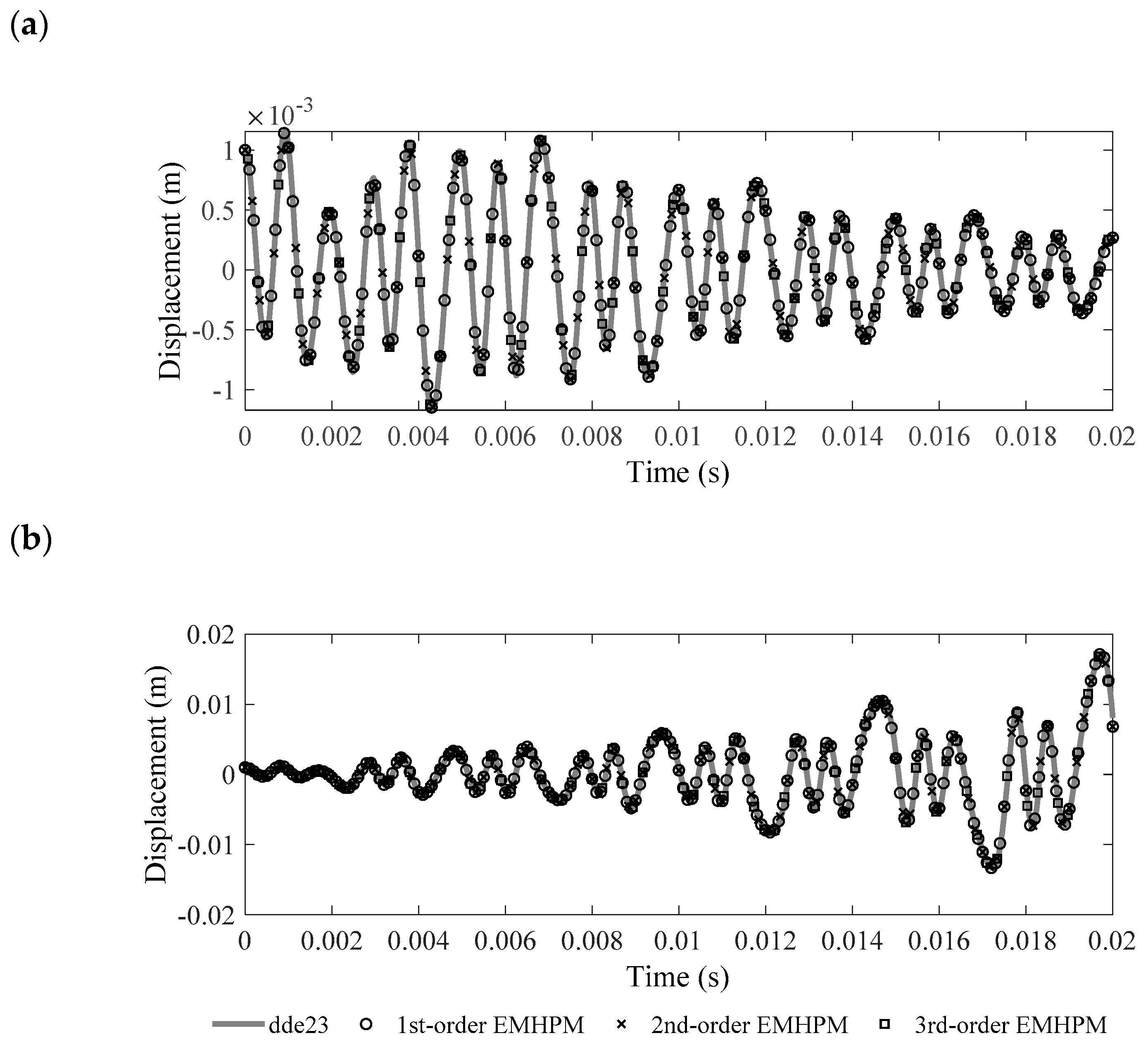
This paper is summarized as follows. Section 2 focuses on the development of second- and third-order EMHPM for stability analysis of DDE. Section 3 studies the application of the second- and third-order EMHPM on the milling equation to demonstrate its improvement in the convergence rate. Section 4 is focused on the use of the third-order EMHPM to compute the stability analysis in milling for multivariable tools, and theoretical predictions with time-domain simulations are performed. Finally, some conclusions are drawn.

2. Enhanced Multistage Homotopy Perturbation Method

2.1. Second-Order EMHPM

Olvera et al. enhanced in [33] the multistage homotopy perturbation method (MHPM) proposed by Hashim [41]. The EMHPM considers the general case in which the nonlinear equation contains terms of the independent variable. This method is also useful to solve an n-dimensional DDE in the state-space form

$$\dot{x}\left(t\right)=A\left(t\right)x+B\left(t\right)x\left(t-\tau \right)$$

(1)

where $A\left(t+\tau \right)=A\left(t\right),B\left(t+\tau \right)=B\left(t\right),x\left(t\right)$, is the state vector, and $\tau$ is the time delay. Equation (1) can be written equivalently as:

$${\dot{x}}_i\left(T\right)-A_t{x}_i\left(T\right)\approx B_t{x}_i{}^{\tau }\left(T\right)$$

(2)

where $x_i\left(T\right)$ indicates the $m$-order solution for Equation (1) that satisfies the initial conditions $x_i\left(0\right)=x_{i-1}$, $A_t$ and $B_t$ are the periodic matrix whose values vary with time $t$. In [42], Puma et al. applied the first-order EMHPM to estimate the delayed term $x_i^{\tau }\left(T\right)$ in Equation (2), in which the period $\left[t_0-\tau ,t_0\right]$ was discretized in $N$ equally spaced discrete state values, and the function that describes the delayed term $x_i^{\tau }\left(T\right)$ in the delayed interval $\left[t_{i-N},t_{i-N+1}\right]$ was approximated as a first-order polynomial representation. Defining $x_i\equiv x_i\left(T\right)$ to simplify the notation, Equation (2) can be written as

$${\dot{x}}_i\left(T\right)=A_t{x}_i(T)+B_t\left(x_{i-N}+\frac{N-1}{\tau }\left(x_{i-N+1}-x_{i-N}\right)T\right)$$

(3)

Figure 1a shows the representation of the approximation of the delayed term with the first-order polynomial. In the second-order EMHPM, to approximate the function that describes the delayed term $x_i^{\tau }\left(T\right)$ in Equation (2), the Lagrange equation is used, making use of the discrete values $x_{i-N},x_{i-N+1},x_{i-N+2}$ as follows:

$$f_n\left(x\right)={\displaystyle \sum _{i=0}^{n}Li\left(x\right)f\left(x_i\right)},L_i\left(x\right)={\displaystyle \prod _{i=0,i\ne k}^n\frac{x-x_i}{x_k-x_i}}$$

(4)

to achieve a second-degree polynomial approximation, we have from Equation (4) that

$$P_2\left(x\right)=\frac{\left(x-\Delta t\right)\left(x-2\Delta t\right)}{\left(0-\Delta t\right)\left(0-2\Delta t\right)}f\left(x_{i-N}\right)+\frac{\left(x-0\right)\left(x-2\Delta t\right)}{\left(\Delta t-0\right)\left(\Delta t-2\Delta t\right)}f\left(x_{i-N+1}\right)+\frac{\left(x-0\right)\left(x-\Delta t\right)}{\left(2\Delta t-0\right)\left(2\Delta t-\Delta t\right)}f\left(x_{i-N+2}\right)$$

(5)

Substituting $x=T$ and $\Delta t=\left(N-1\right)/\tau$, we obtain the function that describes the delayed interval as:

$$x_{i-N+1}\left(T\right)\approx x_{i-N}+\left(\frac{N-1}{\tau }\right)T(-\frac{3}{2}{x}_{i-N}+2x_{i-N+1}-\frac{1}{2}{x}_{i-N+2})+{\left(\frac{N-1}{\tau }\right)}^2\frac{T^2}{2}\left(x_{i-N}-2x_{i-N+1}+x_{i-N+2}\right)$$

(6)

When the delay is approximated by a second-degree polynomial it is called second-order EMHPM and should not be confused with the order of solution $m$ and which is determined by the last deformation taking into account the approximated solution. Notice that a polynomial of the second-degree requires three points. Likewise four points in the case of a third-degree polynomial as shown in Figure 1.

The procedure to calculate the second-order EMHPM solution is based on the EMHPM procedure described in [33]. The solution for second-order EMHPM is recursively expressed of $X_{ik}\left(T\right)$ as

$$X_{ik}=X_{ik}^a+X_{ik}^b+X_{ik}^c,k=1,2,3\dots .$$

(7)

where

$$X_{i0}^a=x_{i-1,} X_{i0}^b=X_{i0}^c=0$$

(8)

and

$$\begin{array}{l}{X}_{ik}^a=\frac{T}{k}\left(A_t{X}_{i(k-1)}^a+g\left(k\right)B_t{x}_{i-N}\right)\\ X_{ik}^b=\frac{T}{k+1}\left(A_t{X}_{i(k-1)}^b+g(k)\left(\frac{N-1}{\tau }\right)B_{t}T\left(-\frac{3}{2}{x}_{i-N}+2x_{i-N+1}-\frac{1}{2}{x}_{i-N+2}\right)\right)\\ X_{ik}^c=\frac{T}{k+2}\left(A_t{X}_{i(k-1)}^c+g(k){\left(\frac{N-1}{\tau }\right)}^2{B}_t\frac{T^2}{2}\left(x_{i-N}-2x_{i-N+1}+x_{i-N+2}\right)\right)\end{array}$$

(9)

So, the solution of Equation (1) is obtained by adding each of the approximations $X_{ik}$ of Equation (7).

$$x_i\left(T\right)\approx {\displaystyle \sum _{k=0}^m{X}_{ik}\left(T\right)}$$

(10)

2.2. Third-Order EMHPM Solution

For the polynomial representation of the third-degree, the function that describes the delayed term $x_i^{\tau }\left(T\right)$ is approximated by a polynomial of order three, then Equation (4) of the Lagrange interpolator is used accordingly. In this case, it is necessary to employ the $x_{i-N},x_{i-N+1},x_{i-N+2}, x_{i-N+3}$ discrete values. Following the same procedure described in Section 2.1, the function that describes the delayed interval is given as:

$$\begin{array}{cc}\hfill x_i^{\tau }\left(T\right)=& x_{i-N+1}\left(T\right)\approx x_{i-N}+\left(\frac{N-1}{\tau }\right)T(-\frac{11}{6}{x}_{i-N}+3x_{i-N+1}-\frac{3}{2}{x}_{i-N+2}+\frac{1}{3}{x}_{i-N+3})+\hfill \\ & {\left(\frac{N-1}{\tau }\right)}^2\frac{T^2}{2}(2x_{i-N}-5x_{i-N+1}+4x_{i-N+2}-x_{i-N+3})+{\left(\frac{N-1}{\tau }\right)}^3\frac{T^3}{6}\left(-x_{i-N}+3x_{i-N+1}-3x_{i-N+2}+x_{i-N+3}\right)\hfill \end{array}$$

(11)

Following the EMHPM procedure, the recursive solution of Equation (1) $X_{ik}\left(T\right)$ is expressed as

$$X_{ik}=X_{ik}^a+X_{ik}^b+X_{ik}^c+X_{ik}^d,k=1,2,3\dots .$$

(12)

where

$$X_{i0}^a=x_{i-1,}{X}_{i0}^b=X_{i0}^c=X_{i0}^d=0$$

(13)

and

$$\begin{array}{l}{X}_{ik}^a=\frac{T}{k}\left(A_t{X}_{i(k-1)}^a+g\left(k\right)B_t{x}_{i-N}\right)\\ X_{ik}^b=\frac{T}{k+1}(A_t{X}_{i(k-1)}^b+g(k)\left(\frac{N-1}{\tau }\right)B_{t}T(-\frac{11}{6}{x}_{i-N}+3x_{i-N+1}-\frac{3}{2}{x}_{i-N+2}+\frac{1}{3}{x}_{i-N+3}))\\ X_{ik}^c=\frac{T}{k+2}(A_t{X}_{i(k-1)}^c+g(k){\left(\frac{N-1}{\tau }\right)}^2{B}_t\frac{T^2}{2}(2x_{i-N}-5x_{i-N+1}+4x_{i-N+2}-x_{i-N+3}))\\ X_{ik}^d=\frac{T}{k+3}(A_t{X}_{i(k-1)}^d+g(k){\left(\frac{N-1}{\tau }\right)}^3{B}_t\frac{T^3}{6}(-x_{i-N}+3x_{i-N+1}-3x_{i-N+2}+x_{i-N+3}))\end{array}$$

(14)

The approximate solution of Equation (1) can be obtained by substituting Equation (12) into Equation (10) adding each of the approximations $X_{ik}$.

2.3. Stability Analysis

To calculate the stability of the differential Equation (1) using the second-order EMHPM, the solution of Equation (10) for second-order EMHPM must be rewritten by grouping each of the discrete values $x_{\mathrm{i}},x_{i-N+2},x_{i-N+1},x_{i-N}$, resulting in

$$x_i(T)\approx P_i(T)x_{i-1}+Q_i{}^{\prime }(T)x_{i-N+2}+Q_i(T)x_{i-N+1}+R_i(T)x_{i-N}$$

(15)

where

$$\begin{array}{l}{P}_i(T)={\displaystyle \sum _{k=0}^m\frac{1}{k!}}{A}_t^k{T}^k,\\ Q{{}^{\prime }}_i(T)={\displaystyle \sum _{k=1}^m\left(\frac{1}{(k+2)!}{\left(\frac{N-1}{\tau }\right)}^2{A}_t^{k-1}{B}_t{T}^{k+2}-\frac{1}{2(k+1)!}\left(\frac{N-1}{\tau }\right)A_t^{k-1}{B}_t{T}^{k+1}\right)}\\ Q_i(T)={\displaystyle \sum _{k=1}^m\frac{1}{(k+1)!}\left(\frac{N-1}{\tau }\right)A_t^{k-1}{B}_t{T}^{k+1}-2Q{{}^{\prime }}_i}\\ R_i(T)={\displaystyle \sum _{k=1}^m\frac{1}{k!}{A}_t^{k-1}{B}_t{T}^k-Q{{}^{\prime }}_i-Q_i}\end{array}$$

(16)

Similarly, to compute the stability lobes for the third-order EMHPM, the solution of the differential Equation (1) for third-order EMHPM is rewritten as

$$x_i(T)\approx P_i(T)x_{i-1}+Q{{}^{″}}_i(T)x_{i-N+3}+Q{{}^{\prime }}_i(T)x_{i-N+2}+Q_i(T)x_{i-N+1}+R_i(T)x_{i-N}$$

(17)

where

$$\begin{array}{l}{P}_i(T)={\displaystyle \sum _{k=0}^m\frac{1}{k!}}{A}_t^k{T}^k,\\ Q{{}^{″}}_i(T)={\displaystyle \sum _{k=1}^m\left(\frac{1}{(k+1)!}\left(\frac{N-1}{\tau }\right)A_t^{k-1}{B}_t{T}^{k+1}\left(\frac{1}{3}\right)-\frac{1}{(k+2)!}{\left(\frac{N-1}{\tau }\right)}^2{A}_t^{k-1}{B}_t{T}^{k+2}+\frac{1}{(k+3)!}{\left(\frac{N-1}{\tau }\right)}^3{A}_t^{k-1}{B}_t{T}^{k+3}\right)}\\ Q{{}^{\prime }}_i(T)={\displaystyle \sum _{k=1}^m\left(\begin{array}{l}\frac{1}{(k+1)!}\left(\frac{N-1}{\tau }\right)A_t^{k-1}{B}_t{T}^{k+1}+\frac{1}{(k+2)!}{\left(\frac{N-1}{\tau }\right)}^2{A}_t^{k-1}{B}_t{T}^{k+2}\left(-\frac{7}{2}\right)\\ +\frac{1}{(k+3)!}{\left(\frac{N-1}{\tau }\right)}^3{A}_t^{k-1}{B}_t{T}^{k+3}\left(\frac{9}{2}\right)\end{array}\right)}-\frac{15}{2}Q{}^{\prime }{{}^{\prime }}_i\\ Q_i(T)={\displaystyle \sum _{k=1}^m\left(\frac{1}{(k+1)!}\left(\frac{N-1}{\tau }\right)A_t^{k-1}{B}_t{T}^{k+1}\right)-3Q{}^{\prime }{{}^{\prime }}_i-2Q{{}^{\prime }}_i}\\ R_i(T)={\displaystyle \sum _{k=1}^m\frac{1}{k!}{A}_t^{k-1}{B}_t{T}^k-Q{}^{\prime }{{}^{\prime }}_i-Q{{}^{\prime }}_i-Q_i}\end{array}$$

(18)

The approximate solution obtained from Equation (17) was used to define a discrete map following the procedure described in [43]:

$$w_i=D_i{w}_{i-1}$$

(19)

where $w_{i-1}$ is a vector with dimension equal to the total number of states (displacement and velocity) for all $N$ discrete intervals:

$$w_{i-1}=[x_{(i-1)},{\dot{x}}_{(i-1)},x_{(i-2)},\dots ,x_{(i-N)}]{ }^T$$

(20)

$D_i$ is a coefficient matrix and for the third-order EMHPM it has the form:

$$D_i=\left[\begin{array}{cccccccccc}P& 0& 0& 0& \cdots & 0& Q{{}^{″}}_i& Q{{}^{\prime }}_i& Q_i& R_i\\ I& 0& 0& 0& \cdots & 0& 0& 0& 0& 0\\ 0& I& 0& 0& \cdots & 0& 0& 0& 0& 0\\ 0& 0& I& 0& \cdots & 0& 0& 0& 0& 0\\ ⋮& ⋮& ⋮& \ddots & ⋮& ⋮& ⋮& ⋮& ⋮& ⋮\\ 0& 0& 0& 0& \ddots & 0& 0& 0& 0& 0\\ 0& 0& 0& 0& \cdots & I& 0& 0& 0& 0\\ 0& 0& 0& 0& \cdots & 0& I& 0& 0& 0\\ 0& 0& 0& 0& \cdots & 0& 0& I& 0& 0\\ 0& 0& 0& 0& \cdots & 0& 0& 0& I& 0\end{array}\right]$$

(21)

It is important to point out that in the case of the second-order EMHPM, the matrix $D_{\mathrm{i}}$ is like the matrix of the third-order EMHPM without the matrix $Q_i^{{}^{″}}$.

Then, the Floquet transition matrix Φ is calculated over the main period $\tau =\left(N-1\right)/\mathsf{\Delta }t$, coupling each of the discrete maps $D_i$, $i=1,2,\dots ,\left(N-1\right),$ to obtain:

$$\Phi =D_{N-1}{D}_{N-2}\dots D_2{D}_1$$

(22)

Thus, the stability of Equation (1) is determined by calculating the eigenvalues of the transition matrix given by Equation (22). The eigenvalues of the transition matrix are actually the Floquet multipliers which are the exponents of each complex exponential functions that describe the motion of Equation (1). If the modulus of greatest magnitude is greater than or equal to one, it implies that the system will behave in an unstable way and the amplitude of the vibration will increase exponentially, otherwise it will have a stable behavior.

3. Numeric Solution of the Milling Equation

3.1. Dynamic Model to the Milling Equation

To validate the proposed EMHPM methods, the numerical solution of the delay differential equation analyzed by Olvera et al., in [33] was calculated, which describes the dynamic model of the milling process in one degree of freedom (DOF):

$$\ddot{x}\left(t\right)+2\zeta {\omega }_n\dot{x}\left(t\right)+{\omega }_n^{2}x(t)=-\frac{a_p{h}_{xx}\left(t\right)}{m_m}\left(x\left(t\right)-x\left(t-\tau \right)\right)$$

(23)

where $\zeta$ is the modal damping ratio, ${\omega }_n$ is the natural frequency of the workpiece, $a_p$ is the axial depth of cut, $m_m$ is the modal mass, $\tau$ represents the time delay corresponding to the hitting period between each tooth of the tool and $h_{xx}\left(t\right)$ is the specific cutting force in the x-direction due to flexibility in x-direction, which was calculated depending on the position of the tool

$$h_{xx}(t)={\displaystyle \sum _{iz=1}^{z_n}g\left({\varphi }_{iz}(t)\right)sin{\varphi }_{iz}(t)\left(K_{tc}\cos {\varphi }_{iz}(t)+K_{nc}\sin {\varphi }_{iz}(t)\right)}$$

(24)

$z_n$ is the number of edges of the tool, $K_{tc}$ and $K_{nc}$ are the average specific cut coefficients in the tangential and normal direction, respectively, and ${\varphi }_{iz}\left(t\right)$ is the angular position of each left edge described by

$${\varphi }_{iz}=\left(2\pi n/60\right)t+2\pi iz/z_n$$

(25)

where $n$ is the spindle speed in revolution per minute (rpm). The function $g\left({\varphi }_{iz}\left(t\right)\right)$ is a window function, which has the value of one when the current edge $iz$ is cutting material, otherwise it takes the value zero.

In up-milling ${\varphi }_{st}=0$and ${\varphi }_{ex}={\cos }^{-1}\left(1-2a_d\right),$ conversely in down-milling ${\varphi }_{st}={\cos }^{-1}\left(2a_d-1\right)$ and ${\varphi }_{ex}=\pi$, $a_d$ is the radial immersion ratio of the cut and ${\varphi }_{st}$and ${\varphi }_{ex}$ are the angular positions where each edge enters and leaves the workpiece.

The second- and third-order EMHPM is applied to obtain the solution of Equation (23) and it is compared with the solution given by the first-order EMHPM [33]; for a regular tool the matrix $A$ and $B$ are represented as:

$$A_t=\left[\begin{array}{cc}0& 1\\ -{\omega }_n^2-\frac{a_p{h}_{xx}(t)}{m_m}& -2\zeta {\omega }_n\end{array}\right], B_t=\left[\begin{array}{cc}0& 0\\ \frac{a_p{h}_{xx}(t)}{m_m}& 0\end{array}\right]$$

(26)

$A_t$ and $B_t$ correspond to the periodic matrix evaluated at time $t$. For demonstration purposes, time-domain simulations were computed for a full-immersion down-milling operation. We used the parameters employed by Insperger et al., in [43] where the stability lobes were also calculated. The modal parameters $f_n$ = 922 Hz, ${\omega }_n=5793$ rad/s, $\zeta =0.011$ and $m_m=0.03993$ kg corresponds to a single degree of freedom. The tangential and normal cutting coefficients are $K_{tc}=6\times {10}^8$ N/${\mathrm{m}}^2$ and $K_{nc}=2\times {10}^8$ N/${\mathrm{m}}^2$ respectively for an end-mill with $z_n=2$. The time-domain solution was computed using the EMHPM considering $N=76$ discrete intervals and $m=7$. Two sets of cutting conditions were chosen for a fixed spindle speed value of $n=12000$ rpm where the axial depth of cut of $a_p=1.5$ mm corresponds to a stable cutting operation while that for an unstable operation $a_p=3$ mm was chosen. In Figure 2 we plot the second- and third-order EMHPM solutions and compare it with the first-order EMHPM and the dde23 routine in Matlab, which is used to integrate DDE.

3.2. Numerical Comparison between Methods

In order to observe the rate of convergence of the first-, second- and third-order EMHPM, we chose the stable case with cutting conditions $a_p=1.5$ mm, $a_d=1$ and n = 12,000 rpm presented in Figure 3a, and the unstable case with cutting conditions $a_p=3$ mm, $a_d=1$ and n = 12,000 rpm showed in Figure 3b. The rate of convergence was analyzed by computing the absolute error between the solution with N discrete intervals and a converged solution. All methods were compared against itself using the solution provided with N = 200 discrete intervals, which are considered the converged solution. In Figure 3a it is observed that the convergence is better for the second- and third-order than the first-order, however, the difference of convergence between second- and third-order with the parameters used was negligible. On the other hand, Figure 3b shows that for few discrete intervals the third-order EMHPM had the fastest convergence in comparison with the second- and the first-order EMHPM. However, the second-order and third-order curves behaved very similarly after N = 50 discrete intervals. It is important to mention that for a typical stability solution in the ranges of spindle speed 5000–10,000 rpm, N = 40 discrete intervals will be enough to have accurate predictions.

Since the rate of convergence was proved for time-domain simulations, we next explored the convergence of the methods applied to the stability analysis. The stability lobes computed with the second- and third-order EMHPM for regular milling tools were compared with its predecessor for radial immersion value of $a_d$ =1 and the other parameters indicated above as it was used in [44]. Figure 4 shows the stability diagrams for spindle speed in the range 2000–3000 rev/min where the precision of the method was compromised due to the higher value of the time delay. While the shaded gray area represents the stability lobes computed with N = 200 discrete intervals in all subfigures, in each subfigure solid black lines draw the stability frontier for a specific discrete interval and using the first-, second- or third-order EMHPM. In Figure 4 the first, second and third column represents the solution for the first-, the second- and the third-order EMHPM respectively, while the first and the second row was for N = 60 and N = 100 discrete intervals, respectively. It is observed that the error achieved in the third-order EMHPM was less than those attained for the first-order and second-order EMHPM solutions. This confirms that the third-order EMHPM had the highest rate of convergence.

The results were also compared, in Figure 4g, with the semi-discretization method (SDM) presented by Insperger and Stépán in [43] (dot line) and with the full-discretization method (FDM) presented by Ding et al. in [45] (dash line). It is observed that the EMHPM converged faster than the SDM and FDM.

Table 1. Comparison of convergence for different methods for down-milling operation with $a_d=1$

Method	$\mathit{N}=60$		$\mathit{N}=100$
	Time (s)	Error	Time (s)	Error
First-order EMHPM	52.39	1.6276	186.35	0.3203
Second-order EMHPM	54.85	0.3507	194.65	0.0568
Third-order EMHPM	61.48	0.3458	195.86	0.0563
FDM	61.26	1.4097	191.49	0.3998
SDM	278.03	-	570.04	-

list the results for computation times for a different number of discretized intervals together with the absolute error between stability frontiers. Notice that the solution obtained with the EMHPM with N = 60 discrete intervals was faster than the SDM and the FDM and even the error was less in the solution by the EMHPM. For N = 100 discrete intervals the computation time for the FDM was similar to the solution obtained with the EMHPM but it was demonstrated that the solution by second- and third-order EMHPM requires a smaller number of discretized intervals to converge to the solution and using a smaller amount of computation time. Notice the error for the SDM was not calculated since there was no stability frontier in some values of spindle speed.

It is noticeable that exists a significant improvement in the rate of convergence from first-order to second-order and third-order EMHPM, however, the difference between the second- and the third-order EMHPM is negligible if the number of discretized intervals increase. There is no best method between second- and third-order EMHPM in terms of rate of convergence and computation time since the precision depends on the nature of the studied problem. However, it is easy to prove that a higher-order approximation (fourth- and fifth-order EMHPM) could drastically increase the computational time without a significant improvement in the solution.

4. Stability Analysis of Multivariable Milling Tools

The EMHPM can be generalized for stability analysis of DDEs having multiple delays. A multivariable tool contains some of the following characteristics: uneven pitch between teeth, and/or at least one helix angle with a different value from the others. This analysis was developed by Compeán et al., in [34] by using the first-order EMHPM, where the methodology for the characterization of the cutting coefficients for a multivariable tool was discussed, and the dynamic behavior was studied from the productivity point of view. Since the angular spacing at the beginning of the edge is different between teeth (pitch) and the different values of helix angles of the edges between adjacent teeth, the angular spacing between teeth at a specific height changes continuously, which produces an infinite number of delays. A common approach to deal with the DDE with an infinite number of delay is to discretize the tool by cutting disks in the axial direction with a thickness $\Delta a_{dsk}$ to induce a DDE with a finite number of delays. A single disk still has the same number of flutes (discrete flutes) and considering that the maximum delay in the process is the period of rotation of the tool or the spindle rotation period ${\tau }_T$, then, it can be discretized in $N-1$ intervals.

The angular position between two adjacent teeth in each cutting disk changes according to the axial position of the referred disk and is related to the expression $\psi =k_{\beta }{a}_p$, where $k_{\beta }=2\tan \beta /2D$. Here $D$ is the diameter of the tool and $\psi$ represents the cutting-edge offset angle due to the helix angle. A certain interval can be associated with a discrete time delay of each tooth $iz$ and disk $l$ using the following formulation

$$N_{iz,l}=round\left((N-1)\frac{\delta {\varphi }_{iz,l}}{2\pi }\right)$$

(27)

where $\delta {\varphi }_{iz,l}$ is the angular pitch between consecutive teeth for each disk, the round function converts the argument to the nearest integer. In Equation (27) $N_{iz}$_, is a table (matrix) of dimension iz × l. Since this procedure could generate several delayed terms and some of them with the same value of discrete time delay due to the discretization scheme, it is required to collect all the different (non-repeated) discrete time delays $d_n$ from $N_{iz,l}$.

Thus, without loss of generality, the DDE with multiple delays can be written as

$$\dot{x}(t)=A(t)x(t)+{\displaystyle \sum _{d=\min \left(d_n\right)}^{\max \left(d_n\right)}{B}^{d}x(t-\tau )}$$

(28)

where x is the vector of states, $A\left(t+{\tau }_T\right)=A\left({\tau }_T\right)$, $B^d\left(t+{\tau }_T\right)=B^d\left({\tau }_T\right)$ and ${\tau }_T$ is the period of rotation of the spindle. Following the EMHPM procedure, Equation (28) can be written equivalently by intervals as:

$${\dot{x}}_i(T)-A_t{x}_i(T)\approx {\displaystyle \sum _{d=\min \left(d_n\right)}^{\max \left(d_n\right)}{B}_t{}^d{x}_i{}^{{\tau }_d}(T)}$$

(29)

being $x_i\left(T\right)$ the solution by intervals of order m for Equation (28) in the $i-th$ interval that satisfies the initial condition $x_i\left(0\right)={\mathrm{x}}_{i-1}$, the matrices $A_t$ and $B_t^d$ represent the values of the matrices $A\left(t\right)$ and $B^d\left(t\right)$ evaluated at time $t$ respectively.

4.1. Third-Order EMHPM for Multivariable Milling Tool

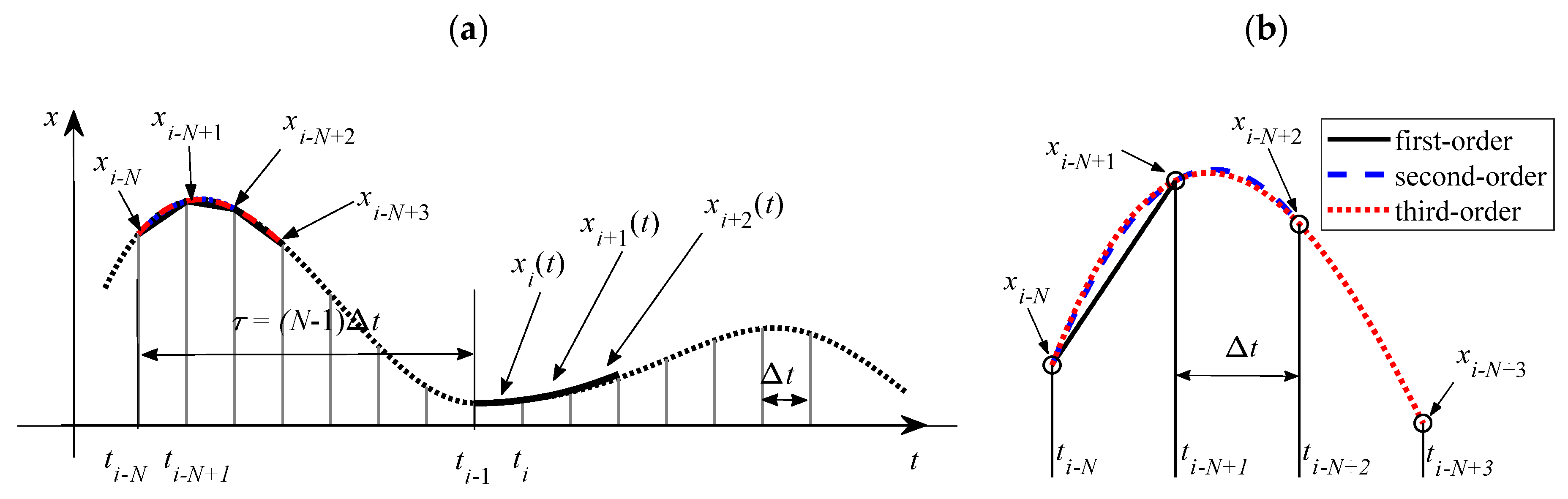
To approximate the term associated with the delayed terms $x_i^{{\tau }_d}\left(T\right)$ of Equation (29), the interval of the period ${\tau }_T,\left[t_0-{\tau }_T,t_0\right]$ is discretized in $N-1$ intervals that can be equal size. For simplicity, intervals of equal size $\Delta t={\tau }_T/\left(N-1\right)$ are chosen. Then it is assumed that the function $x_i^{{\tau }_d}\left(T\right)$, which is defined in the interval $\left[t_{i-d-1},t_{i-d+2}\right],$ for the third-order EMHPM has the representation of the form:

$$\begin{array}{c}{x}_i^{{\tau }_d}\left(T\right)=x_{i-d}\left(T\right)\approx x_{i-d-1}+\left(\frac{N-1}{{\tau }_T}\right)T(-\frac{11}{6}\left(x_{i-d-1}\right)+3\left(x_{i-d}\right)-\frac{3}{2}\left(x_{i-d+1}\right)+\frac{1}{3}\left(x_{i-d+2}\right))+\\ {\left(\frac{N-1}{{\tau }_T}\right)}^2\frac{T^2}{2}\left(2\left(x_{i-d-1}\right)-5\left(x_{i-d}\right)+4\left(x_{i-d+1}\right)-\left(x_{i-d+2}\right)\right)+\\ {\left(\frac{N-1}{{\tau }_T}\right)}^3\frac{T^3}{6}\left(-x_{i-d-1}+3\left(x_{i-d}\right)-3\left(x_{i-d+1}\right)+x_{i-d+2}\right)\end{array}$$

(30)

Defining $x_i\equiv x_i\left(T_i\right)$ to simplify the notation, and substituting Equation (30) in Equation (29), the following equation is obtained:

$${\dot{x}}_i(T)=A_t{x}_i(T)+{\displaystyle \sum _{d=\min \left(d_n\right)}^{\mathrm{m}ax\left(d_n\right)}\left(\begin{array}{l}{B}_t{}^d{x}_{i-d-1}+B_t{}^{d}T\left(\frac{N-1}{{\tau }_T}\right)(-\frac{11}{6}\left(x_{i-d-1}\right)+3\left(x_{i-d}\right)-\frac{3}{2}\left(x_{i-d+1}\right)+\frac{1}{3}\left(x_{i-d+2}\right))+\\ B_t{}^d\frac{T^2}{2}{\left(\frac{N-1}{{\tau }_T}\right)}^2\left(2\left(x_{i-d-1}\right)-5\left(x_{i-d}\right)+4\left(x_{i-d+1}\right)-x_{i-d+2}\right)+\\ B_t{}^d\frac{T^3}{6}{\left(\frac{N-1}{{\tau }_T}\right)}^3\left(-x_{i-d-1}+3\left(x_{i-d}\right)-3\left(x_{i-d+1}\right)+x_{i-d+2}\right)\end{array}\right)}$$

(31)

where

$$A_t=\left[\begin{array}{cc}0& 1\\ -{\omega }_n^2-\frac{\Delta a_{disk}}{m_m}{\displaystyle \sum _{d=\min \left(d_n\right)}^{\max \left(d_n\right)}{h}_{yy}^d}& -2\zeta {\omega }_n\end{array}\right], B_t{}^d=\left[\begin{array}{cc}0& 0\\ \frac{\Delta a_{disk}}{m_m}{\displaystyle \sum _{d=\min \left(d_n\right)}^{\max \left(d_n\right)}{h}_{yy}^d}& 0\end{array}\right]$$

(32)

here, $h_{yy}$ is the specific cutting force in the y-direction due to flexibility in y-direction, which is used for thin wall machining. This force was calculated depending on the position of the tool via the following equation:

$$h_{yy}(t)={\displaystyle \sum _{iz=1}^{z_n}g\left({\varphi }_{iz}(t)\right)\cos {\varphi }_{iz}(t)\left(-K_{tc}\sin {\varphi }_{iz}(t)+K_{nc}\cos {\varphi }_{iz}(t)\right)}$$

(33)

Then, solving Equation (31) yields

$$\begin{array}{l}{X}_{i0}=x_{i-1}\\ X_{i1}=T{A}_t\left(x_{i-1}\right)+{\displaystyle \sum _{d=\min \left(d_n\right)}^{\max \left(d_n\right)}\left(\begin{array}{l}T{B}_t{}^d\left(x_{i-d-1}\right)+B_t{}^d\frac{T^2}{2}\left(\frac{N-1}{{\tau }_T}\right)(-\frac{11}{6}\left(x_{i-d-1}\right)+3\left(x_{i-d}\right)-\frac{3}{2}\left(x_{i-d+1}\right)+\frac{1}{3}\left(x_{i-d+2}\right))\\ +B_t{}^d\frac{T^3}{6}{\left(\frac{N-1}{{\tau }_T}\right)}^2\left(2\left(x_{i-d-1}\right)-5\left(x_{i-d}\right)+4\left(x_{i-d+1}\right)-x_{i-d+2}\right)\\ +B_t{}^d\frac{T^4}{24}{\left(\frac{N-1}{{\tau }_T}\right)}^3\left(-x_{i-d-1}+3\left(x_{i-d}\right)-3\left(x_{i-d+1}\right)+x_{i-d+2}\right)\end{array}\right)}\\ X_{i2}=\frac{T^2}{2}{A}_t{}^2\left(x_{i-1}\right)+A_t{\displaystyle \sum _{d=\min \left(d_n\right)}^{\max \left(d_n\right)}\left(\begin{array}{l}\frac{T^2}{2}{B}_t{}^d\left(x_{i-d-1}\right)+B_t{}^d\frac{T^3}{6}\left(\frac{N-1}{{\tau }_T}\right)(-\frac{11}{6}\left(x_{i-d-1}\right)+3\left(x_{i-d}\right)-\frac{3}{2}\left(x_{i-d+1}\right)+\frac{1}{3}\left(x_{i-d+2}\right))+\\ B_t{}^d\frac{T^4}{24}{\left(\frac{N-1}{{\tau }_T}\right)}^2\left(2\left(x_{i-d-1}\right)-5\left(x_{i-d}\right)+4\left(x_{i-d+1}\right)-x_{i-d+2}\right)+\\ B_t{}^d\frac{T^5}{120}{\left(\frac{N-1}{{\tau }_T}\right)}^3\left(-x_{i-d-1}+3\left(x_{i-d}\right)-3\left(x_{i-d+1}\right)+x_{i-d+2}\right)\end{array}\right)}\\ ⋮\\ X_{ik}=\frac{1}{k!}{T}^k{A}_t{}^k\left(x_{i-1}\right)+A_t{}^{k-1}{\displaystyle \sum _{d=\min \left(d_n\right)}^{\max \left(d_n\right)}\left(\begin{array}{l}\frac{1}{k!}{T}^k{B}_t{}^d\left(x_{i-d-1}\right)+\frac{1}{\left(k+1\right)!}{T}^{k+1}{B}_t{}^d\left(\frac{N-1}{{\tau }_T}\right)(-\frac{11}{6}\left(x_{i-d-1}\right)+3\left(x_{i-d}\right)-\frac{3}{2}\left(x_{i-d+1}\right)+\\ \frac{1}{3}\left(x_{i-d+2}\right))+\frac{1}{\left(k+2\right)!}{T}^{k+2}{B}_t{}^d{\left(\frac{N-1}{{\tau }_T}\right)}^2\left(2\left(x_{i-d-1}\right)-5\left(x_{i-d}\right)+4\left(x_{i-d+1}\right)-x_{i-d+2}\right)+\\ \frac{1}{\left(k+3\right)!}{T}^{k+3}{B}_t{}^d{\left(\frac{N-1}{{\tau }_T}\right)}^3\left(-x_{i-d-1}+3\left(x_{i-d}\right)-3\left(x_{i-d+1}\right)+x_{i-d+2}\right)\end{array}\right)}\end{array}$$

(34)

Notice that Equation (34) can be written recursively as

$$X_{ik}=X_{ik}^a+X_{ik}^b+X_{ik}^c+X_{ik}^d,k=1,2,3\dots .$$

(35)

where $X_{i0}^a=x_{i-1},X_{i0}^b,=X_{i0}^c=X_{i0}^d=0$ and

$$\begin{array}{l}{X}_{ik}^a=\frac{T}{k}\left(A_t{X}_{i(k-1)}^a+g\left(k\right){\displaystyle \sum _{d=\min \left(d_n\right)}^{\max \left(d_n\right)}{B}_t^d{x}_{i-d-1}}\right)\\ X_{ik}^b=\frac{T}{k+1}\left(A_t{X}_{i(k-1)}^b+g(k){\displaystyle \sum _{d=\min \left(d_n\right)}^{\max \left(d_n\right)}\left(\frac{N-1}{\tau }\right)B_t^{d}T(-\frac{11}{6}\left(x_{i-d-1}\right)+3\left(x_{i-d}\right)-\frac{3}{2}\left(x_{i-d+1}\right)+\frac{1}{3}\left(x_{i-d+2}\right))}\right)\\ X_{ik}^c=\frac{T}{k+2}\left(A_t{X}_{i(k-1)}^c+g(k){\displaystyle \sum _{d=\min \left(d_n\right)}^{\max \left(d_n\right)}{\left(\frac{N-1}{\tau }\right)}^2{B}_t^d\frac{T^2}{2}\left(2\left(x_{i-d-1}\right)-5\left(x_{i-d}\right)+4\left(x_{i-d+1}\right)-x_{i-d+2}\right)}\right)\\ X_{ik}^d=\frac{T}{k+3}\left(A_t{X}_{i(k-1)}^d+g(k){\displaystyle \sum _{d=\min \left(d_n\right)}^{\max \left(d_n\right)}{\left(\frac{N-1}{\tau }\right)}^3{B}_t^d\frac{T^3}{6}\left(-x_{i-d-1}+3\left(x_{i-d}\right)-3\left(x_{i-d+1}\right)+x_{i-d+2}\right)}\right)\end{array}$$

(36)

the solution of order $m$ for Equation (31) was obtained by adding each of the approximations $k$ of Equation (35). Similar to Equation (15), to obtain the stability graphs the solution of Equation (35) is rewritten by grouping the discrete states, which results in:

$$x_i(T)\approx P_i(T)x_{(i-1)}+{\displaystyle \sum _{d=\min \left(d_n\right)}^{\max \left(d_n\right)}\left(Q_{{}_i}^{{}^{″}}{}^d(T)x_{i-d+2}+Q_{{}_i}^{{}^{\prime }}{}^d(T)x_{i-d+1}+Q_{{}_i}^d(T)x_{i-d}+R_{{}_i}^d(T)x_{i-d-1}\right)}$$

(37)

where

$$\begin{array}{l}{P}_i(T)={\displaystyle \sum _{k=0}^m\frac{1}{k!}}{A}_t^k{T}^k,\\ Q{ }_i^{{}^{″}d}(T)={\displaystyle \sum _{k=1}^m\left(\begin{array}{l}\frac{1}{(k+1)!}\left(\frac{N-1}{{\tau }_T}\right)A_t^{k-1}{B}_t^d{T}^{k+1}\left(\frac{1}{3}\right)-\frac{1}{(k+2)!}{\left(\frac{N-1}{{\tau }_T}\right)}^2{A}_t^{k-1}{B}_t^d{T}^{k+2}+\\ \frac{1}{(k+3)!}{\left(\frac{N-1}{{\tau }_T}\right)}^3{A}_t^{k-1}{B}_t^d{T}^{k+3}\end{array}\right)}\\ Q_i^{{}^{\prime }d}(T)={\displaystyle \sum _{k=1}^m\left(\begin{array}{l}\frac{1}{(k+1)!}\left(\frac{N-1}{{\tau }_T}\right)A_t^{k-1}{B}_t^d{T}^{k+1}+\frac{1}{(k+2)!}{\left(\frac{N-1}{{\tau }_T}\right)}^2{A}_t^{k-1}{B}_t^d{T}^{k+2}\left(-\frac{7}{2}\right)+\\ \frac{1}{(k+3)!}{\left(\frac{N-1}{{\tau }_T}\right)}^3{A}_t^{k-1}{B}_t^d{T}^{k+3}\left(\frac{9}{2}\right)\end{array}\right)-\frac{15}{2}{Q}_i^{{}^{″}d}}\\ Q_i^d(T)={\displaystyle \sum _{k=1}^m\left(\frac{1}{(k+1)!}\left(\frac{N-1}{{\tau }_T}\right)A_t^{k-1}{B}_t^d{T}^{k+1}\right)-3Q_i^{{}^{″}d}-2Q_i^{{}^{\prime }d}}\\ R_i^d(T)={\displaystyle \sum _{k=1}^m\frac{1}{k!}{A}_t^{k-1}{B}_t^d{T}^k-Q_i^{{}^{″}d}-Q_i^{{}^{\prime }d}-Q_i^d}\end{array}$$

(38)

The approximate solution obtained from Equation (37) was used to define a discrete map:

$$w_i=D_i{w}_{i-1}$$

(39)

where $w_{i-1}$ is a vector represented by Equation (20) and $D_i$ is a coefficient matrix given by

$$D_i=\left[\begin{array}{ccccccccccccccccccc}{P}_i& 0& \cdots & Q_i^{″1}& Q_i^{\prime 1}& Q_i^1& R_i^1& \cdots & Q_i^{″2}& Q_i^{\prime 2}& Q_i^2& R_i^2& \cdots & Q_i^{″d_n}& Q_i^{\prime d_n}& Q_i^{d_n}& R_i^{d_n}& \cdots & 0\\ I& 0& \cdots & 0& 0& 0& 0& \cdots & 0& 0& 0& 0& \cdots & 0& 0& 0& 0& \cdots & 0\\ 0& I& \cdots & 0& 0& 0& 0& \cdots & 0& 0& 0& 0& \cdots & 0& 0& 0& 0& \cdots & 0\\ 0& 0& \ddots & 0& 0& 0& 0& \cdots & 0& 0& 0& 0& \cdots & 0& 0& 0& 0& \cdots & 0\\ ⋮& ⋮& ⋮& I& 0& 0& 0& \cdots & 0& 0& 0& 0& \cdots & 0& 0& 0& 0& \cdots & 0\\ 0& 0& \cdots & 0& I& 0& 0& \cdots & 0& 0& 0& 0& \cdots & 0& 0& 0& 0& \cdots & 0\\ 0& 0& \cdots & 0& 0& I& 0& \cdots & 0& 0& 0& 0& \cdots & 0& 0& 0& 0& \cdots & 0\\ 0& 0& \cdots & 0& 0& 0& I& \cdots & 0& 0& 0& 0& \cdots & 0& 0& 0& 0& \cdots & 0\\ 0& 0& \cdots & 0& 0& 0& 0& \ddots & 0& 0& 0& 0& \cdots & 0& 0& 0& 0& \cdots & 0\\ 0& 0& \cdots & 0& 0& 0& 0& \cdots & I& 0& 0& 0& \cdots & 0& 0& 0& 0& \cdots & 0\\ 0& 0& \cdots & 0& 0& 0& 0& \cdots & 0& I& 0& 0& \cdots & 0& 0& 0& 0& \cdots & 0\\ 0& 0& \cdots & 0& 0& 0& 0& \cdots & 0& 0& I& 0& \cdots & 0& 0& 0& 0& \cdots & 0\\ 0& 0& \cdots & 0& 0& 0& 0& \cdots & 0& 0& 0& I& \cdots & 0& 0& 0& 0& \cdots & 0\\ 0& 0& \cdots & 0& 0& 0& 0& \cdots & 0& 0& 0& 0& \ddots & 0& 0& 0& 0& \cdots & 0\\ 0& 0& \cdots & 0& 0& 0& 0& \cdots & 0& 0& 0& 0& \cdots & I& 0& 0& 0& \cdots & 0\\ 0& 0& \cdots & 0& 0& 0& 0& \cdots & 0& 0& 0& 0& \cdots & 0& I& 0& 0& \cdots & 0\\ 0& 0& \cdots & 0& 0& 0& 0& \cdots & 0& 0& 0& 0& \cdots & 0& 0& I& 0& \cdots & 0\\ ⋮& ⋮& \cdots & ⋮& ⋮& ⋮& ⋮& \cdots & ⋮& ⋮& ⋮& ⋮& \cdots & 0& 0& 0& I& \cdots & ⋮\\ 0& 0& \cdots & 0& 0& 0& 0& \cdots & 0& 0& 0& 0& \cdots & 0& 0& 0& 0& \cdots & 0\end{array}\right]$$

(40)

The transition matrix $\Phi$ over the period ${\tau }_T=\left(N-1\right)/\mathsf{\Delta }t$ was determined by coupling each solution $x_i$ through the discrete map $D_i$, $i=1,2,\dots ,\left(N-1\right)$. However, the computational cost can be reduced by computing only the transition matrix up to the maximum delayed term without losing precision in the calculation of the eigenvalues:

$$\Phi =D_{N\max }{D}_{N\max - 1}\dots D_2{D}_1$$

(41)

Thus, the stability graphs of Equation (28) were determined by computing the eigenvalues of the transition matrix of Equation (41). The results obtained from the EMHPM were corroborated with the stability lobes in the study of multivariate tools [27].

4.2. Experimental Characterization of One Degree of Freedom Milling Equation and Cutting Force Model

4.2.1. Experimental Modal Analysis

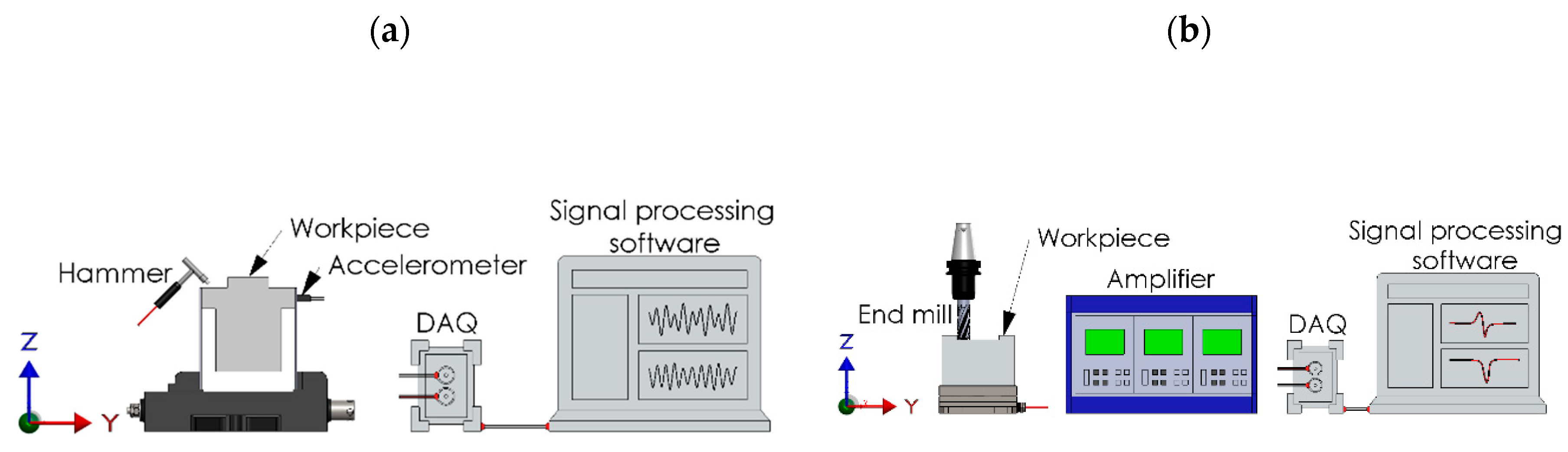
An experimental workpiece was assembled with a 7075T6 aluminum block of 101 mm × 172 mm supported by two thin plates (walls) with a thickness of 4.5 mm. This assembly mimics a DOF as described in Equation (23). The workpiece assembly was rigidly fixed to the workbench of a Makino F3 machining center. For modal analysis, tap testing was performed using a 352C68 PCB Piezotronics accelerometer and an impact hammer model 9722A500. The signals were acquired with a Polytec VIB-E-220 data acquisition card and processed with VibSoft signal analyzer software as shown in Figure 5a. Using the CutPro 8 software, the modal parameters were fitted resulting the values $\zeta =0.068$, $m_m=3.8$ kg, $f_m$ = 132 Hz and ${\omega }_n=829$rad/s.

4.2.2. Experimental Determination of Cutting Coefficients

The force model in Equation (33) was used to predict the cutting force magnitude for a given depth of cut. It is based on a mechanistic approach that assumes a relationship between forces and the uncut chip thickness by means of the cutting coefficients. The cutting force model was established by introducing cutting (shearing) and edge coefficients for the tangential and normal directions of the milling tool. The characterization procedure assumed the linear relationship between the averaged experimental cutting forces $\tilde{F}$ and the feed rate f_z in x- and y- directions. This relationship is established as follows:

$$\tilde{F}=f_z{\tilde{F}}_c+{\tilde{F}}_e$$

(42)

Here, $\widetilde{F_c}$ and $\widetilde{F_e}$ are the cutting shear and edge components, respectively. The experimental forces at each feed rate are measured, and the cutting-edge components $\widetilde{F_c}$ and $\widetilde{F_e}$ were evaluated

$$K_{tc}=4\frac{{\tilde{F}}_{yc}}{z_n{a}_p}, K_{nc}=-4\frac{{\tilde{F}}_{xc}}{z_n{a}_p}$$

(43)

A multivariable cutter provided by a local toolmaker was characterized by using Equation (43) and the experimental setup shown in Figure 5b.

Table 2. Main geometric parameters of multivariable tool.

	Diameter	12.7 mm
	Cutting length	25 mm
	Coating type	Uncoated
	Number of teeth	4
	Helix angles	39°, 37°, 39°, 41°
	Pitch angles	80°, 100°, 70°, 110°

summarizes the main geometric characteristics of the multivariable tool. A total of five cuttings were performed for full radial immersion in aluminum 7075T6 during dry machining. The forces were recorded by using a dynamometer 9257B Kistler and the spindle speed was set at 3000 rpm based on the dynamometer’s natural frequency to avoid the amplification of milling forces. The force signals were acquired using a VibSoft-20 acquisition card at a sample rate of 48 kHz and processed in a custom-made MATLAB app to remove drift and noise. Cutting forces data were collected for the axial depth of cut of 2 mm and four values of feed per tooth 0.05, 0.10, 0.015 and 0.20, so the resulting cutting coefficients $K_{tc}$for the tooth 1, 2, 3 and 4 were $1215\times {10}^6,$ 1$369\times {10}^6,$ $897\times {10}^6$and $1799\times {10}^6$ N/${\mathrm{m}}^2$ respectively, while that the coefficients $K_{nc}$ for the tooth 1, 2, 3 and 4 resulted $272\times {10}^6,$ $520\times {10}^6$, $801\times {10}^6$ and $859\times {10}^6$ N/${\mathrm{m}}^2$ respectively.

4.3. Stability Analysis of 1 DOF Milling with a Multivariable Tool

The stability lobes computed for the multivariable tool using the third-order EMHPM with a mesh of $400\times 200$ ($n\times a_p$) are shown in Figure 6 together with stability lobes for a regular tool (angles of 90° and helix angles of 30° for all flutes). An approximation of order $m=7$ was used with N = 241 and $a_d=1$ mm. Notice from Figure 6 that the stable zone obtained for the multivariable tool was significantly larger, meaning that the critical depth of cut was higher in most spindle speeds, which allowed having more global productivity. It is also observed in the range of spindle speed between 2000 and 3000 rpm, a stable peninsula formed with axial depth ranging from 11 to 20 mm or higher values of critical depth of cut. For instance, for the multivariable cutter at 2500 rpm, the critical depth of cut $a_p$ was 2.17 mm, however it became stable again as shown in Figure 6 for the interval values between 11 and 20 mm. To validate this unexpected behavior, we performed several time-domain simulations using the third-order EMHPM solution described by Equation (37).

Furthermore, the simulated vibrations for the chosen cutting conditions were analyzed using the continuous wavelet transform (CWT), the power spectral density (PSD) and Poincaré maps (PM). The CWT is a time-frequency representation of a signal that offers the capability to observe how frequencies evolve in time. The scalograms display the absolute value of CWT of the simulated vibration and therefore, they were used to detect chatter phenomena that appeared when milling with a multivariable tool. The PSD is based on the Fourier transform that provides the transformation from the time-domain to the frequency-domain. Additionally, PSD is defined as the squared value of the signal and describes the power of a signal or time series distributed over different frequencies [46]. Moreover, a PM represents points in phase space, which are sampled every spindle rotation [47]. The frequencies $f$ of the CWT and PM were normalized $f_n=f/f_h$ according to the spindle frequency $f_h$. When milling with a regular milling tool the excitation frequency $f_e$ is equal to $z_n$ times frequencies of the spindle speed $f_h$ but in a multivariable tool, there are several excitation frequencies since the angular spacing between teeth change as a function of the axial depth of cut.

Figure 7 illustrates the CWT, PSD and PM for simulated vibrations using the multivariable tool with different axial depths denoted as cutting conditions A, B and C for the axial depths of cut of 1.0, 1.7 and 1.7 mm respectively. Figure 7a–c refers to the vibrations of the cutting conditions A marked in Figure 6, using a regular tool. The scalogram in Figure 7a identifies point A as a stable cutting since normalized cutting frequencies present a dominant value of $f_n$ = 3.2, which corresponds to the natural frequency $f_m=132$ Hz. This is also confirmed by the PSD analysis shown in Figure 7b. The PM illustrated in Figure 7c shows a vibration that decreased with time and sampled data concentrated in the center confirmed a typical stable case. When the axial depth of cut was increased to 1.7 mm, the stability diagram predicted unstable cutting conditions according to the stability lobes for the regular tool. This case is denoted with cutting conditions B and the corresponding scalogram (shown in Figure 7d) illustrated how the intensity of the dominant frequency increased with time even when the excitation frequency was the same as the case in A.

The PM diagram shown in Figure 7f exhibited a vibration far from zero. In fact, the PM diagram shows that the vibration amplitude grows exponentially because our equation of motion did not consider nonlinear effects such as those that appeared when the tool lost contact with the workpiece. Both cutting conditions A and B agreed with the stability boundaries in Figure 6. Now, the cutting conditions B were used but with a multivariable tool, which was referred to as cutting conditions C. The CWT plotted in Figure 7g described completely different results since there were no single dominant frequencies in comparison with cutting conditions A, but appeared several frequencies around $f_n$ = 3.2 and close to $f_n$ = 1 that reduced in intensity with time, suggesting a stable cutting. Figure 7i illustrates how the vibration amplitude approached to zero when using a multivariable tool in contrast to the PM obtained for the regular tool and exhibited in Figure 7f. This can be explained by observing that there were several excitation frequencies due to the irregular pitch and helix angles that break a single excitation frequency avoiding regenerative chatter phenomena.

Figure 8 illustrates the CWT, PSD and PM for simulated vibrations using the multivariable tool with different axial depths denoted as cutting conditions D, E, F and G for the axial depths of cut of 2.3, 3.0, 8.55 and 18 mm respectively. Notice that a stable case C was already validated when the axial depth was 1.7 mm in Figure 7g–i that corresponded to cutting conditions under the stability boundaries shown in Figure 6. For case D, a transient cutting condition was chosen very close to the critical axial depth of the cut. It is interesting to point out that transition cutting conditions in the CWT scalogram shown in Figure 8a not only shows frequencies with higher intensity in comparison with the stable case B, but also presents shifted frequencies that varied in intensity every single revolution. This shifting suggests a marginally stable cutting condition that was confirmed by the PM illustrated in Figure 8c, where circular trajectories were described close to the center point.

Unstable vibrations that appeared for case E were because of the intensity of frequencies increased exponentially with time, see Figure 8d. Notice that other frequencies arose with time close to the values of $f_n$ = 0.5 and $f_n$ = 1.5. These frenquencies also occurred for cutting conditions D, which is an indication of the appearance of chatter phenomena. In contrast to Figure 7i for a stable case, Figure 8f exhibited few trajectories because the vibration amplitude was out of the range selected (±1 mm). The qualitative and quantitative dynamic behaviour due to cutting conditions F, and illustrated in Figure 8g-i, were classified as transition cutting behaviour. Here, a more severe shifting in frequencies was observed in the scalogram (Figure 8g). From Figure 8g, it is seen that drastic shifting occurred in the time domain in the range of normalized frequencies from 3.5 to 6. It was also evident in the PM showed in Figure 8i, that the amplitude of vibration remained below 1 mm during several revolutions of the tool but the amplitude of vibration never aproached to the center point, in contrast to the stable cutting condition C shown in Figure 7i in which the oscillation aplitudes aproached the center.

An interesting dynamic behaviour was observed in the milling cutting process when the cutting conditions were selected in the middle of the stable peninsula, above unstable cutting conditions such as E cutting conditions. The axial depth of the cut was increased from the unstable axial depth of cut of 3–18 mm, 6 times higher of the stable cutting condition C and 2 times higher than the unstable condition E. Since the vibration quickly decreased in a few revolutions no dominant frequencies appeared in the CWT and PSD failed to clearly identify a dominant frequency since the vibration amplitude decreased to zero after few revolutions, as confirmed by the PM shown in Figure 8l.

Figure 9 shows the normalized excitation frequencies that the multivariable tool produced for a fixed spindle speed of 2500 rpm. The total number of disks of 50 μm of thickness was grouped in sets of each millimeter in the axial direction. The waterfall plot in Figure 9 explains that a stable peninsula was formed above 11 mm because the workpiece was excited with several frequencies simultaneously. For instance, for a milling operation with the axial depth of cut of 1 mm (stable cutting), 80 discrete disks were cut with four normalized excitation frequencies values (3.3, 3.6, 4.5 and 5.1). On the other hand, when milling at 18 mm (stable cutting), there were 14 normalized excitation frequencies (3.30, 3.35, 3.39, 3.44, 3.49, 3.54, 3.60, 4.55, 4.64, 4.73, 4.82, 4.92, 5.02 and 5.13), most of them with at least 115 discrete disks.

5. Conclusions

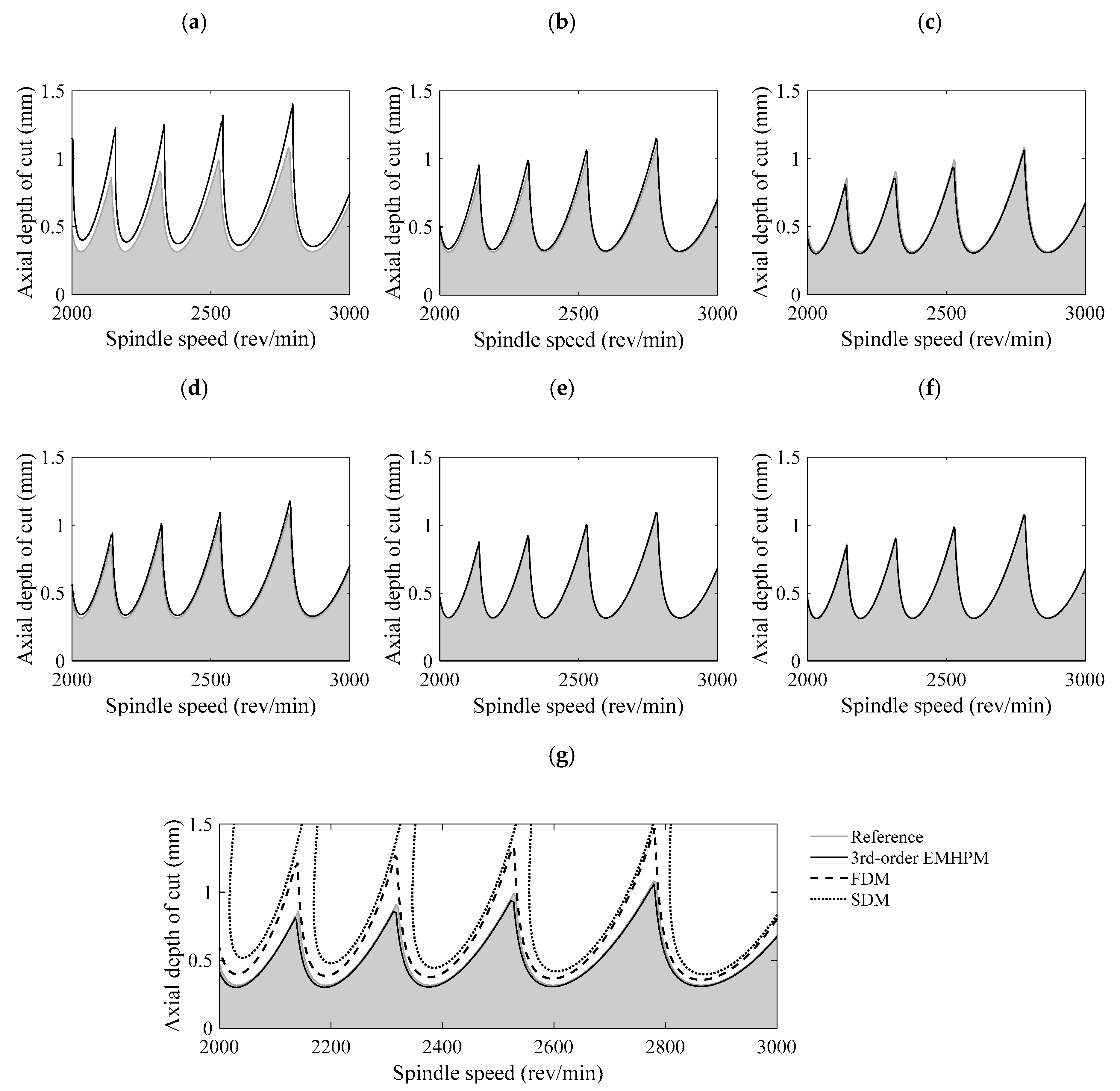
In this work, quadratic and cubic polynomials were used to approximate the delayed terms of delay differential equations. Numerical simulations showed that using second- and third-order EMHPM improved the convergence rate and required less computational time when compared to the first-order EMHPM, and to semi-discretization and full-discretization methods, since fewer approximations or less discrete intervals were needed to reduce the computation time.

To further assess the applicability of the proposed method, the third-order EMHPM was used for determining the stability bounds in one-degree-of-freedom milling operation with a multivariable tool, demonstrating that the stability zone improved in comparison with a regular tool. For instance, at 2500 rpm the critical axial depth of the cut was 1.3 mm using the regular milling tool. However, using the multivariable tool, the critical axial depth of the cut was increased until 2.17 mm but more interesting, a stable zone appeared above 8.55 mm.

The CWT scalograms, PSD charts and PM were employed to validate the stability lobes found by using the third-order EMHPM for the multivariable tool. Numerical solutions confirmed the system dynamics behavior predicted by the third-order EMHPM.

Based on the above results, this paper provided evidence the third-order EMHPM could be used to study dynamic phenomena that appeared at higher axial depths of cut due to the multivariable design of the tool, which broke the excitation frequencies at a lower depth of cut.

References

1. Mi, T.; Chen, N.; Stepan, G.; Takacs, D. Energy distribution of a vehicle shimmy system with the delayed tyre model. IFAC-PapersOnLine 2018, 51, 7–12. [Google Scholar] [CrossRef]
2. Orosz, G.; Stépán, G. Subcritical hopf bifurcations in a car-following model with reaction-time delay. Proc. R. Soc. A Math. Phys. Eng. Sci. 2006, 462, 2643–2670. [Google Scholar] [CrossRef] [Green Version]
3. Hu, H.; Zaihua, W. Dynamics of Controlled Mechanical Systems with Delayed Feedback; Springer Science & Business Media: Berlin, Germany, 2002; ISBN 9783642078392. [Google Scholar]
4. Altintas, Y. Manufacturing Automation. Metal Cutting Mechanics, Machine Tool Vibrations, and CNC Design; Cambridge University Press: New York, NY, USA, 2012. [Google Scholar]
5. Kuljanic, E.; Totis, G.; Sortino, M. Development of an intelligent multisensor chatter detection system in milling. Mech. Syst. Signal Process. 2009, 23, 1704–1718. [Google Scholar] [CrossRef]
6. Zhuo, Y.; Jin, H.; Han, Z. Chatter identification in flank milling of thin-walled blade based on fractal dimension. Procedia Manuf. 2020, 49, 150–154. [Google Scholar] [CrossRef]
7. Paul, S.; Morales-Menendez, R. Chatter mitigation in milling process using discrete time sliding mode control with type 2-fuzzy logic system. Appl. Sci. 2019, 9, 4380. [Google Scholar] [CrossRef] [Green Version]
8. Peng, C.; Wang, L.; Liao, T.W. A new method for the prediction of chatter stability lobes based on dynamic cutting force simulation model and support vector machine. J. Sound Vib. 2015, 354, 118–131. [Google Scholar] [CrossRef]
9. Li, D.; Cao, H.; Chen, X. Fuzzy control of milling chatter with piezoelectric actuators embedded to the tool holder. Mech. Syst. Signal Process. 2020, 148, 107190. [Google Scholar] [CrossRef]
10. Wan, S.; Li, X.; Su, W.; Yuan, J.; Hong, J.; Jin, X. Active damping of milling chatter vibration via a novel spindle system with an integrated electromagnetic actuator. Precis. Eng. 2019, 57, 203–210. [Google Scholar] [CrossRef]
11. Munoa, J.; Sanz-Calle, M.; Dombovari, Z.; Iglesias, A.; Pena-Barrio, J.; Stepan, G. Tuneable clamping table for chatter avoidance in thin-walled part milling. CIRP Ann. 2020, 69, 313–316. [Google Scholar] [CrossRef]
12. Wang, Y.; Wang, T.; Yu, Z.; Zhang, Y.; Wang, Y.; Liu, H. Chatter prediction for variable pitch and variable helix milling. Shock Vib. 2015, 2015. [Google Scholar] [CrossRef]
13. Mei, Y.; Mo, R.; Sun, H.; He, B.; Bu, K. Stability analysis of milling process with multiple delays. Appl. Sci. 2020, 10, 3646. [Google Scholar] [CrossRef]
14. Wan, M.; Zhang, W.H.; Dang, J.W.; Yang, Y. A unified stability prediction method for milling process with multiple delays. Int. J. Mach. Tools Manuf. 2010, 50, 29–41. [Google Scholar] [CrossRef]
15. Zhan, D.; Jiang, S.; Niu, J.; Sun, Y. Dynamics modeling and stability analysis of five-axis ball-end milling system with variable pitch tools. Int. J. Mech. Sci. 2020, 182, 105774. [Google Scholar] [CrossRef]
16. Slavicek, J. The effect of irregular tooth pitch on stability of milling. Proc. 6th MTDR Conf. 1965, 1, 15–22. [Google Scholar]
17. Budak, E. An analytical design method for milling cutters with nonconstant pitch to increase stability, Part I: Theory. J. Manuf. Sci. Eng. Trans. ASME 2003, 125, 29–34. [Google Scholar] [CrossRef]
18. Budak, E. An analytical design method for milling cutters with nonconstant pitch to increase stability, Part 2: Application. J. Manuf. Sci. Eng. Trans. ASME 2003, 125, 35–38. [Google Scholar] [CrossRef] [Green Version]
19. Altintas, Y.; Engin, S.; Budak, E. Analytical stability prediction and design of variable pitch cutters. J. Manuf. Sci. Eng. Trans. ASME 1999, 121, 173–178. [Google Scholar] [CrossRef]
20. Olgac, N.; Sipahi, R. Dynamics and stability of variable-pitch milling. J. Vib. Control 2007, 13, 1031–1043. [Google Scholar] [CrossRef]
21. Jin, G.; Zhang, Q.; Hao, S.; Xie, Q. Stability prediction of milling process with variable pitch cutter. Math. Probl. Eng. 2013, 2013. [Google Scholar] [CrossRef] [Green Version]
22. Comak, A.; Budak, E. Modeling dynamics and stability of variable pitch and helix milling tools for development of a design method to maximize chatter stability. Precis. Eng. 2017, 47, 459–468. [Google Scholar] [CrossRef]
23. Zatarain, M.; Muñoa, J.; Peigne, G.; Insperger, T. Analysis of the influence of mill helix angle on chatter stability. CIRP Ann. Manuf. Technol. 2006, 55, 365–368. [Google Scholar] [CrossRef]
24. Budak, E.; Altintas, Y. Analytical prediction of chatter stability in milling—Part I: General formulation. Am. Soc. Mech. Eng. Dyn. Syst. Meas. Control 1998, 120, 22–30. [Google Scholar] [CrossRef]
25. Insperger, T.; Muñoa, J.; Zatarain, M.; Peigné, G. Unstable islands in the stability chart of milling processes due to the helix angle. In Proceedings of the CIRP 2nd International Conference High Performance Cutting, Vancouver, BC, Canada, 12–13 June 2006. [Google Scholar]
26. Patel, B.R.; Mann, B.P.; Young, K.A. Uncharted islands of chatter instability in milling. Int. J. Mach. Tools Manuf. 2008, 48, 124–134. [Google Scholar] [CrossRef]
27. Sims, N.D.; Mann, B.; Huyanan, S. Analytical prediction of chatter stability for variable pitch and variable helix milling tools. J. Sound Vib. 2008, 317, 664–686. [Google Scholar] [CrossRef] [Green Version]
28. Turner, S.; Merdol, D.; Altintas, Y.; Ridgway, K. Modelling of the stability of variable helix end mills. Int. J. Mach. Tools Manuf. 2007, 47, 1410–1416. [Google Scholar] [CrossRef]
29. Yusoff, A.R.; Sims, N.D. Optimisation of variable helix tool geometry for regenerative chatter mitigation. Int. J. Mach. Tools Manuf. 2011, 51, 133–141. [Google Scholar] [CrossRef] [Green Version]
30. Dombovari, Z.; Stepan, G. The effect of helix angle variation on milling stability. J. Manuf. Sci. Eng. Trans. ASME 2012, 134. [Google Scholar] [CrossRef]
31. Huang, J.; Deng, P.; Li, H.; Wen, B. Stability analysis for milling system with variable pitch cutters under variable speed. J. Vibroeng. 2019, 21, 331–347. [Google Scholar] [CrossRef]
32. Cai, S.; Yao, B.; Feng, W.; Cai, Z.; Chen, B.; He, Z. Milling process simulation for the variable pitch cutter based on an integrated process-machine model. Int. J. Adv. Manuf. Technol. 2020, 106, 2779–2791. [Google Scholar] [CrossRef]
33. Olvera, D.; Elías-Zúñiga, A.; López De Lacalle, L.N.; Rodríguez, C.A. Approximate solutions of delay differential equations with constant and variable coefficients by the enhanced multistage homotopy perturbation method. Abstr. Appl. Anal. 2015, 1–12. [Google Scholar] [CrossRef] [Green Version]
34. Compeán, F.I.; Olvera, D.; Campa, F.J.; López De Lacalle, L.N.; Elías-Zúñiga, A.; Rodríguez, C.A. Characterization and stability analysis of a multivariable milling tool by the enhanced multistage homotopy perturbation method. Int. J. Mach. Tools Manuf. 2012, 57, 27–33. [Google Scholar] [CrossRef]
35. Sims, N.D. Fast chatter stability prediction for variable helix milling tools. Proc. Inst. Mech. Eng. Part C J. Mech. Eng. Sci. 2016, 230, 133–144. [Google Scholar] [CrossRef] [Green Version]
36. Otto, A.; Rauh, S.; Ihlenfeldt, S.; Radons, G. Stability of milling with non-uniform pitch and variable helix Tools. Int. J. Adv. Manuf. Technol. 2017, 89, 2613–2625. [Google Scholar] [CrossRef]
37. Niu, J.; Ding, Y.; Zhu, L.M.; Ding, H. Mechanics and multi-regenerative stability of variable pitch and variable helix milling tools considering runout. Int. J. Mach. Tools Manuf. 2017, 123, 129–145. [Google Scholar] [CrossRef]
38. Olvera, D.; Urbikain, G.; Elías-Zuñiga, A.; López de Lacalle, L.N. Improving stability prediction in peripheral milling of Al7075T6. Appl. Sci. 2018, 8, 1316. [Google Scholar] [CrossRef] [Green Version]
39. Iglesias, A.; Dombovari, Z.; Gonzalez, G.; Munoa, J.; Stepan, G. Optimum selection of variable pitch for chatter suppression in face milling operations. Materials 2018, 12, 112. [Google Scholar] [CrossRef] [PubMed] [Green Version]
40. Guo, Y.; Lin, B.; Wang, W. Optimization of variable helix cutter for improving chatter stability. Int. J. Adv. Manuf. Technol. 2019, 104, 2553–2565. [Google Scholar] [CrossRef]
41. Hashim, I.; Chowdhury, M.S.H. Adaptation of homotopy-perturbation method for numeric-analytic solution of system of ODEs. Phys. Lett. Sect. A 2008, 372, 470–481. [Google Scholar] [CrossRef]
42. Puma-Araujo, S.D.; Olvera-Trejo, D.; Martínez-Romero, O.; Urbikain, G.; Elías-Zúñiga, A.; Lacalle, L.N.L. de Semi-active magnetorheological damper device for chatter mitigation during milling of thin-floor components. Appl. Sci. 2020, 10, 5313. [Google Scholar] [CrossRef]
43. Insperger, T.; Stépán, G. Updated semi-discretization method for periodic delay-differential equations with discrete delay. Int. J. Numer. Methods Eng. 2004, 61, 117–141. [Google Scholar] [CrossRef]
44. Insperger, T. Full-discretization and semi-discretization for milling stability prediction: Some comments. Int. J. Mach. Tools Manuf. 2010, 50, 658–662. [Google Scholar] [CrossRef]
45. Ding, Y.; Zhu, L.M.; Zhang, X.J.; Ding, H. A full-discretization method for prediction of milling stability. Int. J. Mach. Tools Manuf. 2010, 50, 502–509. [Google Scholar] [CrossRef]
46. Lee, E.T.; Eun, H.C. Structural damage detection by power spectral density estimation using output-only measurement. Shock Vib. 2016, 2016. [Google Scholar] [CrossRef] [Green Version]
47. Fries, R.H. Fundamentals of Vibrations; Waveland Press: Long Grove, IL, USA, 2000; ISBN 9781482270372. [Google Scholar]
Figure 1. (a) Scheme for the approximation of the delayed term by a first-order (solid black line), second-order (dashed blue line) and third-order (dotted red line) polynomial: (b) zoom in the time interval [ t i N + 1 ,   t i N + 3 ].
Applsci 10 07869 g001
Figure 2. Numerical comparison of the enhanced homotopy perturbation method (EMHPM) solutions of the milling equation, Equation (23), with the dde23 MATLAB routine. (a) Stable milling operation with a p = 1.5 mm, a d = 1 and n = 12000 rpm and (b) unstable milling operation with a p = 3 mm, a d = 1 and n = 12000 rpm.
Applsci 10 07869 g002
Figure 3. Convergence rate of absolute error between first-, second- and third-order EMHPM for down-milling operation. Cutting parameters for (a) a p = 1.5   mm ,   a d = 1 and n = 12000   rpm and (b) a p = 3   mm ,   a d = 1 and n = 12000   rpm .
Applsci 10 07869 g003
Figure 4. Stability diagrams for down-milling operation. The first (ac) and second (df) rows of subfigures correspond to N = 60 and N = 100 discrete intervals, respectively. First (a,d), second (b,e) and third (c,f) columns correspond to the first-, second- and third-order EMHPM, respectively. Subfigure (g) shows a comparison between the third-order EMHPM (black line), the SDM (dot line) and the FDM (dash line) with N = 60 discrete intervals.
Applsci 10 07869 g004
Figure 5. Scheme of the experimental setup for (a) the modal analysis and (b) cutting forces characterization.
Applsci 10 07869 g005
Figure 6. (a) Comparison of stability lobes for regular (black solid line) and multivariable (red solid line) cutters by using the third-order EMHPM and (b) zoom in on chosen cutting conditions for time-domain simulations. The selected points are marked as follows: unstable (cross mark), stable (circle mark) and transition (plus mark) cutting conditions.
Applsci 10 07869 g006
Figure 7. Analysis of cutting conditions A, B and C. Continuous wavelet transform (CWT) scalograms: (a,d,g); power spectral density (PSD): (b,e,h) and Poincaré maps (PM): (c,f,i) corresponds to the cutting conditions A, B and C respectively.
Applsci 10 07869 g007
Figure 8. Analysis of cutting conditions D, E, F and G. CWT scalogram:s (a,d,g,j); PSD: (b,e,h,k) and PM: (c,f,i,l) corresponds to the cutting conditions D, E, F and G respectively.
Applsci 10 07869 g008aApplsci 10 07869 g008b
Figure 9. The number of discrete disks and discrete excitation frequencies as a function of the axial depth of cut for the multivariable tool.
Applsci 10 07869 g009