Article

Continuous Genetic Algorithms in the Optimization of Logistic Networks: Applicability Assessment and Tuning

by
Przemysław Ignaciuk
and
Łukasz Wieczorek
*
Institute of Information Technology, Lodz University of Technology, 215 Wólczańska St., 90-924 Łódź, Poland
*
Author to whom correspondence should be addressed.
Appl. Sci. 2020, 10(21), 7851; https://doi.org/10.3390/app10217851
Submission received: 20 September 2020 / Revised: 23 October 2020 / Accepted: 3 November 2020 / Published: 5 November 2020
(This article belongs to the Section Computing and Artificial Intelligence)

Abstract

:

Featured Application

Cost-efficient resource distribution in modern logistic networks with complex, realistic topologies, i.e., encompassing lateral trans-shipments, delayed replenishments, and uncertain demand placed at any node.

Abstract

Globalization opens up new perspectives for handling goods distribution in logistic networks. However, establishing an efficient inventory policy is challenging by virtue of the analytical and computational complexity. In this study, the goods distribution process that was governed by the order-up-to policy, implemented in either a distributed or centralized way, was investigated in the logistic systems with complex interconnection topologies. Uncertain demand may be imposed at any node, not just at conveniently chosen contact points, with a lost-sales assumption that introduces a non-linearity into the node dynamics. In order to adjust the policy parameters, the continuous genetic algorithm (CGA) was applied, with the fitness function incorporating both the operational costs and customer satisfaction level. This study investigated how to select the parameters of the popular inventory management policy when operating in the non-trivial networked structures. Moreover, precise guidelines for the CGA tuning in the considered class of problems were provided and evaluated in extensive numerical experiments.

1. Introduction

One of the key areas of economic and entrepreneurship activity in modern production-inventory systems, irrespective of the scale, i.e., regional or international, is logistics. Nevertheless, the current conditions in which the logistic companies operate, highly influenced by globalization, make the processes associated with the goods distribution and transportation difficult to analyze formally in precise terms. They are also not amenable to the standard optimization methods due to the high computational complexity. In fact, most of the scientific research in the field until now has focused on the basic configurations, such as single-stage systems [1,2], serial chain [3,4], and tree-like structures [5,6,7]. Meanwhile, in real systems, more complex configurations in the form of logistic networks have been established [8]. The non-linearities, delays, and couplings in the network node interaction typically do not permit obtaining a closed-form solution to the associated optimization problem. Moreover, the traditional models and numerical methods, e.g., involving the Markov chains, are hardly applicable to the actual, high-dimensional cases [9]. Similarly, the application of heuristics requires precise development for a specific scenario and type of network [10]. As an alternative, one might consider customizing artificial intelligence (AI) approaches to complex logistic systems [11,12]. Even though the exact solution may not always be attained with the desired accuracy, the relieved computational and implementation burden provided by a properly tuned AI method makes it an attractive choice for practical management problems.
According to Min [11], the recent literature displays an increasing interest in the AI approaches for process optimization in logistics. The fundamental AI methods, such as agent-based systems, expert systems, and fuzzy logic, find a wide range of applications in the decision-making problems related to scheduling processes. In addition, more sophisticated approaches, such as evolutionary algorithms, have been gradually employed in the planning stage of real-life systems in which the space of potential solutions should be considered in order to find the optimum [13]. These methods, depending on their specifics and implementation choices, can solve a given optimization problem by self-adjusting to the changes in the system variables and constraints. Among other promising approaches one can also point out machine learning, which finds relatively widespread acceptance in the industrial framework [14], and simulation-based optimization [15,16]. The computational intelligence approach is recommended for complex systems in which the optimal solution cannot be formulated in an analytical way, e.g., owing to model non-linearities, and the evaluation of the fitness function requires substantial resources and is time-consuming [17].
Among the attractive AI methods, genetic algorithms (GAs) are relatively well investigated regarding general optimization problems. They form a kind of metaheuristics based on the phenomenon of biological evolution that explores the space of alternative problem solutions to reach the best one, which is quantified through a predefined fitness function [18]. Nowadays, GAs are increasingly used in real-life problems. Jauhar and Pant [19] and Lee [20] note that despite the invention of numerous modern soft computing techniques, GAs are still widely used by scientists in optimization problems. Besides industrial applications, many organizational challenges might be addressed using GAs, e.g., traffic flow control [21]. These real-life problems require a different implementation and tuning philosophy of GAs compared to the benchmark ones due to the substantial computational investment in assessing the population fitness [18]. In order to obtain a solution in a reasonable time, the number of fitness function evaluations needs to be greatly constrained compared to the benchmark cases.
This study investigated the application of GAs for optimizing the goods flow process in logistic networks with a complex, fully-connected topology. The goods distribution was governed by the order-up-to (OUT) inventory policy:
  • Taken in its classical form [22], i.e., implemented in a distributed way, with each node preserving a full local autonomy regarding taking the ordering decisions,
  • Its centralized, networked (NOUT) version [23], which is deployed under the auspices of a common organization governing the network.
The optimization objective was to adjust the policy parameters (reference stock levels at the controlled nodes) such that the holding costs were minimized, while maintaining a specified service level in the presence of time-varying, uncertain demand. The value of the fitness function was obtained by investigating the system’s response to various demand patterns, which required intensive computational effort, as is typical of real-life optimization problems. The policy parameters have a continuous range. Thus, in contrast to the standard–binary–GA form, the application of continuous GAs (CGAs) was considered. This study’s contribution is thus twofold:
  • Investigate how to adjust the parameters of the popular inventory management policy when operating in a complex networked structure such that the cost and service level objectives are attained.
  • Show how to select the CGA parameters for the task of optimizing the logistic network performance, which requires significant computational effort to evaluate the population fitness owing to non-trivial node interaction and the uncertain nature of the demand.
The paper is organized in the following way. First, a literature review related to configuring the classical inventory management policy and tuning the soft computing techniques for efficient performance in the considered class of problems is conducted in Section 2. Then, in Section 3, the system model is introduced and presented in a form that is convenient for computer implementation. The inventory policies are expressed using the model variables in a vector form. Next, in Section 4, the characteristics of CGAs and a way that they can be implemented for solving the problems related to the dynamic goods distribution in logistic networks are discussed. The CGA’s numerical performance is examined in Section 5. Section 6 comprises the discussion of the results and the conclusions.

2. Related Works

The cost-efficient application of an inventory management policy requires setting appropriate parameter values [24]. In the case of the OUT policy, one needs to adjust the reference stock level (RSL) such that excessive operational costs and a loss of customer satisfaction are avoided, which is challenging in networked systems, as the RSLs should be chosen for all the nodes simultaneously. Until now, the policy tuning has been analyzed mostly in the systems with serial and arborescent topologies [25]. For instance, Basten and Houtum [26] studied near-optimal heuristics in serial production systems with backordering. Chang and Lu [27] investigated a similar model, yet with the loss of unsatisfied demand being accounted for. They applied a phase-type approximation with a given cost structure to determine the optimal node RSLs under various fill-rate requirements. Albrecht [28], in turn, presented a decomposition methodology to reconfigure the networked structure into a collection of two-stage subsystems, and in this way, simplified the selection of RSLs. The proposed solution, however, did not take the fixed costs into account. Next, Wang [29] analyzed a two-echelon inventory system that was subjected to a Poisson demand and proposed a heuristic with a reduced computational footprint. However, he considered identical retailers (nodes with the same demand imposed on them). Guerrero et al. [30] extended that model to cover multi-product distribution in the context of the healthcare industry. Then, Eruguz et al. [31] proposed a sequential optimization procedure for five-echelon chains. However, their methodology needed substantial computational effort to tackle the intricacies of the general acyclic multi-echelon systems. Afterward, Avci and Selim [32] developed a numerical framework that enables one to determine safety stock levels in a two-echelon configuration, while allowing for flexibility in choosing the produced goods quantity. However, that framework ensures meeting the holding cost objectives and premium freight performance only for a one-supplier–multiple-retailers model without trans-shipments. Horng and Lin [33] proposed an ordinal optimization-based metaheuristic algorithm for a similar system with multiple suppliers, which displayed improved computational performance. Yet again, the interconnection structure did not allow for the flow of resources between retailers. Afterward, Feng et al. [34] studied a two-stage system with trans-shipments between retailers under uncertain demand, albeit with the investigated topology enforcing a single supplier that replenishes all the retailers at the second stage. Dominguez et al. [35] considered the impact of various structural configurations on the supply chain performance. They revealed the sensitivity of complex distribution networks to rapid and unpredictable demand changes. However, the numerical studies were limited to serial and arborescent configurations only. Ignaciuk and Bartoszewicz [36] investigated optimal control with a quadratic performance index in multi-supplier systems with an arborescent topology. Their control law is an improvement over the OUT policy with respect to demand variance smoothening in the markets that are subjected to significant fluctuations. Recent publications in this category target mostly real-life cases where arborescent models may be applied [37]. However, in the face of globalization, modern logistic systems are organized into mesh-type topologies with arbitrary interconnection architectures. The structural simplifications were found to be ill-suited for these kinds of systems [8], as they lead to undesirable side-effects, e.g., loss of economic gain and customer trust. The policy tuning in more elaborate cases of practical significance, especially in multi-echelon networks, is at an early stage though [38], and requires a detailed study [39]. In particular, in networked systems, unlike serial and arborescent simplifications, distributed vs. centralized policy tuning may lead to drastic cost differences, as evidenced in this work.
While desirable for enriching the knowledge about supply system functionality, formal studies are difficult to conduct on more realistic models that cover inherent uncertainties and non-linearities. Consequently, numerical optimization has been proposed as an alternative to searching for optimal solutions. Chu et al. [6] proposed a framework for setting the optimal reorder points and order quantities in tree-like distribution networks. Ivanov [40] studied the impact of disruption propagation in light of the ripple effect in multi-stage supply chains. Song et al. [41] developed an agent-based simulation system to support multi-project scheduling and decision-making processes. Unfortunately, numerous simulations implicate significant computational time and effort due to the high mathematical complexity of real-life problem descriptions. As a remedy to the dimensionality obstacle, the AI techniques are being proposed, e.g., particle swarm optimization in three-echelon systems [42]. However, GAs are probably the most thoroughly investigated, both theoretically and applied in many real-life situations. Ko et al. [13] considered over 150 publications concerning the AI methods used in manufacturing management, order fulfillment, vehicle routing problems, etc., stressing the popularity and usefulness of GAs. In this line of research, Koulouriotis et al. [43] applied GA-based optimization to obtain suitable control parameters in serial distribution systems with backordering. Then, Paul and Rajendran [44] showed how to adjust RSLs and review periods in divergent two-stage supply chains with a single distributor and multiple retailers. Ambekar and Kapoor [45], in turn, investigated food grain distribution systems with arborescent topologies. Moreover, Senoussi et al. [46], after the analysis of several GA-based heuristics for two-echelon systems, pointed out the crossover and mutation operations as crucial operations that are used to tune non-linear models. Meanwhile, GAs have found a variety of applications in real-life transportation problems. For instance, Pal and Kant [47] proposed a GA-based framework to solve the fuel-efficient problem in smart urban areas for both people transport and perishable goods delivery. Murali et al. [48] combined integer programming with GA for the integrated routing and scheduling of freight trains in large-scale systems. Deng et al. [49] considered the feeder-bus network design problem involving multiple criteria, i.e., service costs, lead-time delays, and the intensity of feeder buses. Zhou et al. [50] adopted GAs to solve the pallet dispatching problem in order to minimize multiple partial costs encompassing transportation, inventory, lease, and losses. Furthermore, GAs may support the goods distribution impacted by various uncertainties, such as pre- or post-disaster times [51,52]. Other nature-inspired techniques, e.g., the whale optimization algorithm [53] or a GA combined with immune algorithms [54], do not yet have a sufficiently well-developed theoretical basis for studying their mechanics and limitations.
The modern inventory management systems exhibit complex interactions, which are neither well-understood analytically, nor exhaustively examined numerically. This work explored how CGAs could be tuned with respect to the selection of population size, selection and recombination methods, mutation probability, etc., to obtain high efficiency when solving optimization problems in modern logistic networks with non-trivial topologies subjected to the popular OUT policy control.

3. System Model

3.1. Problem Statement and Preliminaries

In this work, the process of goods distribution realized in complex, mesh-type logistic networks was analyzed analytically and numerically to obtain efficient performance according to formally defined criteria. The system topology assumed neither limitations nor simplifications in the way the interconnection structure was formed. The uncertain demand may be imposed on any controlled node, with the lost-sales assumption, i.e., no backordering was allowed. The flow of goods among the nodes was governed by the OUT inventory policy implemented in either a distributed or centralized way. Table 1 groups the symbols and notation used in the model description.

3.2. System Actors and Their Relationships

The class of logistic networks under consideration encompasses the structures consisting of N controlled nodes ni, i ∈ ΘN = {1, 2, …, N}, and M external sources mj, j ∈ ΘM = {1, 2, …, M}. The nodes form a mesh interconnection topology with a predetermined direction of goods flow. The demand, whose future evolution is unknown at the instant of taking the goods distribution decision, can be placed at any controlled node. The nodes have a finite storage capacity, whereas the external sources are assumed to not have such a capacity. The sources do not receive customer demand, rather they are used to replenish the stock of controlled nodes. The node interconnections are unidirectional, characterized by a pair of attributes (αij, βij), where:
  • αij is the supplier fraction (SF), which designates how much of the current lot requested by node nj is to be obtained from node ni, αij ∈ [0, 1].
  • βij is the lead-time delay (LTD), which is the time of order completion and shipment from node ni to node nj, βij ∈ [1, Β], where B denotes the maximum LTD between any two directly connected nodes.
The analyzed class of networks does not permit isolated nodes (with no connection to other nodes or external sources) or nodes that would supply the stock for themselves.
The network dynamics are considered within T equally-spaced periods, given as an index through the independent variable t = 0, 1, 2, …, T. The on-hand stock level of node i at time t is denoted by li(t), the external demand imposed on this node is denoted by di(t), and the satisfied one is denoted by si(t). Figure 1 illustrates the sequence of operations occurring at the controlled node in each period, where solid and dashed lines represent the flow of goods and information, respectively.
Let Ω i S ( t ) and Ω i R ( t ) denote the quantity of goods sent and received by node i in period t, respectively. Introducing oi(t) as the amount of goods to be ordered by node i at the end of period t from its suppliers (both from other controlled nodes within the network and the external sources), the quantity of goods sent by node i can be expressed as:
Ω i S ( t )   = j Θ α ij ( t ) o j ( t ) .
Introducing the combined set of indices Θ   =   Θ N     Θ M , the quantity of goods received by node i in period t may be written as:
Ω i R ( t )   = j Θ α ji ( t     β ji ) o i ( t     β ji ) .
Consequently, using (1) and (2), the stock level evolution can be described by
l i ( t   +   1 )   = ( l i ( t )   +   Ω i R ( t )     d i ( t ) ) +   Ω i S ( t ) ,
where ()+ is the saturation function restricting the argument to non-negative values. This function presents a major non-linearity in the considered class of lost-sales systems. With the demand that is actually satisfied by node i at time t denoted by:
s i ( t )   =   min { l i ( t )   +   Ω i R ( t ) ,   d i ( t ) } ,
the stock level evolution can be expressed through the following relationship:
l i ( t   +   1 )   =   l i ( t )   +   Ω i R ( t )     s i ( t )   Ω i S ( t ) .
In the nominal state, each node is able to fulfill both the external demand and internal orders originating from other controlled nodes. However, when the external demand is satisfied, yet the stock is insufficient to complete the internal orders, their quantity is accordingly reduced, leading to yet another capacity restriction:
i 0 j Θ α ji ( t )   1 .
The external sources, which are not subject to capacity limitations, are always able to fulfill all the orders placed by the controlled nodes.

3.3. State-Space Representation

In order to facilitate both the formal analysis and computer implementation, a state-space model was introduced. According to (5), the dynamical dependencies in the considered network may be grouped into:
  l ( t   +   1 )   =   l ( t )   + β = 1 Β M β ( t     β ) o ( t     β ) +   M 0 ( t ) o ( t )     s ( t ) ,
where:
  • l(t) is the vector of on-hand stock levels.
  • s(t) is the vector of satisfied demands.
  • o(t) is the vector of stock replenishment orders.
  • M0(t) is the hollow matrix representing the internal trans-shipments:
M 0 ( t ) = [ 0 α 12 ( t ) α 1 N ( t ) α 21 ( t ) 0 α 2 N ( t ) α N 1 ( t ) α N 2 ( t ) 0 ] .
  • Mβ(t) are the diagonal matrices describing the node interconnections, i.e., for each β ∈ [1, Β]:
M β ( t ) = [ i : β i 1 = β α i 1 ( t ) 0 0 0 i : β i 2 = β α i 2 ( t ) 0 0 0 i : β iN = β α iN ( t ) ] .
For the sake of further derivations, a matrix M is defined as (with the time reference dropped to indicate the nominal operating conditions):
  M   = β = 1 Β M β =   I N   +   M 0 ,
where IN is an identity matrix of size N × N. M is invertible and one can show [55] that M–1 is a positive matrix.

3.4. Order-Up-To Policy

The OUT policy is one of the classical inventory control strategies considered in logistic applications. It aims at maintaining the stock, which is depleted to satisfy the demand imposed at the controlled node, at a chosen RSL. In each period, any controlled node governed according to the OUT policy checks its inventory position, which comprises the sum of the on-hand stock level and the amount of goods in transit, against its RSL. If the inventory position is below the RSL, the node will issue a replenishment order for its suppliers. The fundamental aspect of the OUT policy operation is thus to determine an appropriate RSL for each controlled node. The choice should enable one to satisfy the external demand, while simultaneously avoiding excessive stock accumulation. The standard OUT policy is assumed to be deployed in a distributed way, i.e., independently at each node, and each node may be subjected to the uncertain external demand.
The stock replenishment process at a node (and thus the goods redistribution in the network) proceeds as a sequence of activities to be executed in each period (Figure 1):
  • Register the shipments obtained from the node suppliers (external sources and neighbors in the network).
  • Fulfill the external demand, if possible.
  • Fulfill the orders originating from other nodes in the network, if possible.
  • Based on the discrepancy between the current stock and the RSL, generate a stock replenishment order.
Let l i r be the RSL of node i and Δi(t) denote the amount of goods in transit that are expected at this node. Then, according to the OUT policy, the amount of goods that should be ordered at the end of period t by node i from its suppliers is given by:
o i ( t )   =   l i r     l i ( t )     Δ i ( t ) .
Introducing l r as the vector of RSLs of all the controlled nodes, (11) may be written for the entire network as:
  o ( t )   =   l r   l ( t )   β = 1 Β k = t β t 1 M β ( k ) o ( k ) .
During the optimization process discussed in the numerical section, RSLs will be sought such that a high service level (high satisfaction of the external demand) is guaranteed, while at the same time, excessive stock accumulation is avoided. As is customary in the subject literature [22], the service level is defined as the percentage of fulfilled demand with respect to the requests imposed externally on the network, i.e., the fill rate. It can be shown (see [55] for derivation details) that a 100% fill rate can be obtained with a sufficiently large, precisely determined RSL, even for the highest demand in the entire planning horizon. For such a “worst-case” scenario, the RSL vector is calculated using:
l r   =   ( I N   + β = 1 Β β M β ) M 1 d max ,
where dmax is the vector of the demand upper bounds. However, the value obtained using (13) overestimates the RSLs for time-varying demands. Therefore, in practice, one should adjust lr for a particular type of demand profile, e.g., as analyzed in this work, through the simulations incorporating a CGA.

3.5. Networked Order-Up-To Policy

In contrast to the classical OUT strategy, the NOUT policy takes advantage of the network’s structural knowledge to influence the goods reflow and obtain a cost reduction. The orders are generated using:
  o ( t )   =   M 1 ( l net r     l ( t )   β = 1 Β k = t β t 1 M β ( k ) o ( k ) ) ,
where l net r is a vector grouping RSLs for the NOUT policy. According to [23], the theoretical lower bound for reaching a 100% fill rate under the worst-case conditions is:
l net r   =   ( I N   + β = 1 Β β M β M 1 ) d max .
Comparing (13) with (15), yields:
l r     l net r = ( M 1     I N ) d max = ( ( I N     ( M 0 ) 1 ) 1   I N ) d max = ( I N   +   ( M 0 )   +   ( M 0 ) 2   +       I N ) d max = (   ( M 0 )   +   ( M 0 ) 2   +   ) d max     0 ,
which indicates lower RSLs and smaller holding costs when using the (centralized) NOUT policy with respect to the classical (distributed) one. Similarly to the classical OUT policy, though, one needs to numerically determine the vector of RSLs for efficient performance in the presence of uncertain, stochastic demand that is imposed at the controlled nodes.

4. GA Application in Goods Distribution Systems

Although GAs are used in a relatively wide range of applications in real-life problems, it is difficult to determine the best solution from the candidate set due to the large search space and intensive computational effort used for the fitness evaluation. Therefore, a key point in real-life systems is proper customization (see Simon [18]). For this purpose, one should identify the factors influencing the evolution toward the optimal solution in a limited time (limited number of fitness function evaluations), as well as the system constraints. Sometimes, approximations and simplifications need to be introduced to leverage computational effort vs. the quality and fidelity of the obtained results.

4.1. Introductory Considerations

Typically, in the GA implementations, the objects in the search domain are represented in a binary form. In the case of logistic networks, however, since the search domain occupies a continuous spectrum, it is more appropriate to use a CGA. Second, the choice of the fitness function itself should allow one to assess, with due accuracy, a large number of situations that might occur in the problem area. As part of the evolution, one seeks a propitious balance between elevating customer satisfaction and reducing operational costs. Since in the systems under consideration, the future demand is assumed to be unknown at the moment of taking the stock replenishment decision (as in the practical systems), the fitness value will be determined from a simulation of network behavior for a given demand pattern and repeated many times to reach statistically relevant results.
The next sections treat the structure of the applied CGA depicted in Figure 2 in detail. The recommended parameter configuration is summarized in Table 6.

4.2. System Setting

In order to apply a GA to the considered class of systems, a mapping between the logistic and GA entities needs to be established. It is assumed that:
  • The vector of RSLs reflects an individual in the population. Consequently, the stock level at a controlled node will correspond to the chromosomes in a given individual.
  • Since the domain of inventory stock levels is continuous (any value from the assumed range can form an individual), a CGA is employed instead of a binary-form GA.
  • The fitness function value is obtained via numerical simulations of the system behavior, which is in response to the control inputs established either according to (12) (classical, distributed policy) or (14) (networked, centralized policy).

4.3. Initialization

In the first step, the vector of initial stock levels is calculated according to (15), i.e., assuming the worst-case conditions of a persistent maximum uncertainty (demand). The simulation of network performance using this vector allows one to determine the largest holding cost, i.e., HCmax, and establish the initial population. At the same time, the calculated vector of RSLs constitutes the upper bound of the search space with respect to the chromosome-related operations, i.e., RSL ∈ [0, RSLmax] (component-wise). Therefore, in contrast to the general GA-based computing problems, the initialization is not random, but rather expert-guided.
In order to determine a suitable number of individuals in the population, various population sizes were examined. Table 2 contains the results of over 103 simulations performed for the same distribution scenario assuming different sizes. In the considered class of systems, a 10-individual population allowed for obtaining a high value for the fitness function in a relatively short time.
The performed numerical experiments showed that the fitness function value changed quickly in the initial phase of the optimization run, but less frequently afterward. Then, a sudden improvement of the fitness value may cause a short uptrend; however, the longer the time without changes, the higher the probability that the optimal solution has already been obtained. For this reason, two stop conditions were applied: an overall limit on the number of generations and a limit on the number of generations without fitness value improvements.

4.4. Fitness Function

The fitness function allows one to assess the quality of a particular candidate solution and consequently select the best one from the current population. According to the introductory considerations regarding the considered problem area (Section 3.1), the fitness function should reflect at least two measures of the system’s performance:
  • The goods holding cost HC, HC ∈ [0, HCmax], which quantifies the internal efficiency regarding goods redistribution.
  • The fill rate FR, where FR ∈ [0, 1], which quantifies the system interaction with the external actors that generate the demand.
The following fitness function was considered:
Ψ = ( 1     H C H C max ) γ F R φ ,
where γ and φ are the tuning coefficients that facilitated prioritization of the costs vs. customer satisfaction. By increasing γ, one opts for throttling the capital costs as a primary optimization objective. Meanwhile, setting a larger φ value emphasizes the importance of the system’s external image, i.e., how well it responds to the market demand imposed on the network nodes. Moreover, in order to simplify the calculations and avoid the scaling problem, the performance measures are normalized. For this purpose, the holding cost is divided by its maximal value, i.e., HCmax, which is established via the initial simulation with an overestimated safety stock. As a result, HC/HCmax will be confined to the range [0, 1]. The fill rate, by definition, is always between 0 and 1.

4.5. Selection

Mating and recombination are crucial steps for creating a new population of individuals, as well as the overall GA performance [18]. In our study, numerous selection and crossover techniques were examined, e.g., roulette wheel selection or stochastic universal sampling. Ultimately, the four-way tournament method was chosen since it provided the fastest convergence with a given accuracy for typically-encountered network topologies. Table 3 presents the fitness function values obtained in the CGA-based optimization of a given goods distribution system with different selection methods. The data indicated a significant advantage of the tournament selection over other methods regarding adjusting the policy parameters of networked logistic systems.
The applied method assumed a random selection of four individuals from the source population and designates the fittest one as a parent. This operation was repeated P times for a population of P individuals. An example iteration of the four-way tournament selection in a P-size population is illustrated in Figure 3.

4.6. Crossover

The recombination is performed through a crossover operation. In a given generation, a pair of RSL vectors (individuals) is used to create a pair of new vectors (children) by exchanging the genetic material in the form of the currently adjusted RSLs for a subset of nodes. Table 4 illustrates the influence of different crossover methods on the results of the CGA-based optimization in networked logistic systems. Accordingly, in the considered implementation, a multipoint crossover method was applied. This method consists of swapping the segments lying between uniformly distributed random points for each pair of parent individuals. The two-point crossover operation, employed in the implemented CGA (using more points did not improve the results, whereas it augmented the computations time) is illustrated in Figure 4. Two children are formed by swapping the segments of chromosomes between points X and Y, such that X, Y ∈ [0, N] and XY in individuals C and D.

4.7. Mutation

In order to avoid premature convergence and explore diverse areas of the search space, a mutation operation was performed as the final phase before proceeding to the next generation in the evolution process (Figure 2). As in biology, this might lead to an exceptionally well-adapted (fit) individual, yet should not occur too frequently to avoid erratic behavior. In the CGA, the mutation implies replacing a given chromosome (the current RSL corresponding to the chosen network node) by a random value within the search domain. With the mutation probability set to 0.15, each chromosome in the candidate solution had a 15% chance that its value will be swapped with a random value from the interval [0, RSLmax] established for that node in the initial simulation. In order to adjust the mutation probability, values from a relatively large range of 0–0.5 were considered. The results are summarized in Table 5.

4.8. CGA Summary

In order to facilitate the application of the CGA in the optimization of logistic networks, the choice of algorithm components and parameters, as discussed in Section 4.4, Section 4.5, Section 4.6 and Section 4.7, is summarized in Table 6. The numerical values reflect the recommended setting for obtaining a fast convergence, i.e., a reduced number of fitness function evaluations dictated by the significant computational effort that is invested in simulating the network behavior.

5. Numerical Study

In order to perform a detailed analysis of the goods distribution process and CGA performance in logistic networks, a dedicated, multithreading application has been developed. As the first step in the program, a state-space model was created. The model was parametrized with:
  • A simulation interval.
  • The number of nodes.
  • The type of inventory control strategy used to steer the goods distribution process.
  • The type of statistical distribution used for generating demand requests.
Once the fitness function coefficients were input, the optimizer sought the best vector of RSLs using either a full search method or a CGA. Owing to the large space of potential solutions, which grows exponentially with the number of nodes involved:
l 1 r δ · l 2 r δ · · l N r δ ,
where δ denotes the iteration granularity, the full-search method is feasible only for small networks.

5.1. CGA vs. Monte Carlo (MC) Method

The CGA performance was compared with two benchmark methods. The first one was a full-search algorithm, which can be utilized only in non-sophisticated structures due to the large computational effort. Another, which can verify more complex cases, assumed the performance of MC simulations based on the same parameters as the CGA. In this section, the results obtained through the GA-based optimization are compared with the MC simulations, as is typical in the initial examination of evolutionary algorithms [18].
The MC method operates on the stochastic RSL vectors established in each generation. In contrast to the GA, the fitness evaluation does not assume other evolutionary operations, i.e., selection, crossover, or mutation. The fitness function values are calculated for all the candidate solutions from the generated population. Hence, the subsequent populations do not arise from the previous ones, like in GA-based algorithms, but are arbitrary and independent of each other. The comparison performed in this section tracked the fitness function improvements in the process of the goods distribution using MC simulations and the CGA for 1.5 × 10³ generations, without other stop conditions. In the numerical analysis, three topologies, assuming different network sizes and customer demands, were applied. The simulation horizon was set to 30 periods. Each population of candidate solutions, both for the CGA and MC simulations, contained 10 individuals. The mutation probability for the CGA was set to 15%. The first examined topology encompassed five nodes (N = 3, M = 2), which led to 1.7 × 10⁸ candidate solutions to examine the full-search algorithm with the same granularity set for all methods. The second topology comprised 14 nodes (N = 10, M = 4), with a search space of 4.8 × 1029 solutions, which was no longer feasible for the full-search approach. Finally, the last network comprised 27 nodes (N = 21, M = 6), which translated to 2 × 1069 possibilities for forming an RSL vector. Table 7 summarizes the results obtained for these three networks.
The data gathered in Table 7 shows the effectiveness of the considered CGA and its superiority over the MC simulations. The evolutionary method achieved the goals set by the network managers in a short time. The conducted tests allow one to observe two significant aspects of GA-based optimization in the resource distribution environments under consideration. The first one concerns the size of the network topology: the bigger the interconnection structure, the greater the savings that are obtained using the GA-based optimization relative to the MC one. Owing to the relatively small search space, the results of the five-node network were similar for both methods. By exploring a large amount of the search space, the MC method had a bigger probability of finding a good solution than in the remaining two cases of more complex topologies. For the larger search spaces, correspondingly, for the fourteen- and twenty-seven-node topologies, the CGA found much better solutions. The CGA was more efficient at finding good solutions in the case of polarized priority in the objective function (either γ or φ set to be much larger than the other coefficient). The plots presented in Figure 5 depict the improvements in the fitness function value obtained using the CGA vs. the MC method for the twenty-seven-node topology. Figure 5a–c illustrates the optimization process convergence for the fitness function coefficients that were adjusted to (γ = 1, φ = 1), (γ = 1, φ = 10), and (γ = 10, φ = 10), respectively. All the cases showed that CGA allowed one to find the optimal solution in a smaller number of iterations than the MC approach. This is a key observation for the analyzed class of real-life systems, which require high computational investments when determining a single fitness function value.
The execution of the optimization procedure with the CGA lasted on average 45, 311, and 1268 s for the five-, fourteen-, and twenty-seven-node networks, respectively. Thus, the computation time grew exponentially with the network size, albeit linearly with the planning horizon. The CGA performance in this aspect may yet be improved, e.g., by recurring using the hardware-assisted parallelization techniques [56].

5.2. The CGA in the Inventory Policy Optimization

In order to comment on the usefulness of the CGA regarding optimizing logistic network behavior, numerous models with topologies of different sizes and complexities were examined (number of nodes: 5–70; gamma, Poisson, normal distributions with different parameters; around 5000 problem instances overall). For illustrative purposes, two representative examples were selected and given detailed treatments in the latter part of this section. The first series of these simulations was conducted in the framework of a “small” network comprising five nodes (N = 3, M = 2) and was compared with the exact solution obtained using the full-search approach. The second example corresponded to a much larger, fourteen-node system (N = 10, M = 4), which was not amenable to the exhaustive-search method. The common parameters were set as follows:
  • Simulation interval T = 50 periods.
  • External demand was imposed on all the controlled nodes, which was generated using a gamma distribution with the shape and scale coefficients equal to 5 and 10, respectively.
  • The CGA population comprised 10 individuals.
  • Mutation probability = 15%.
  • Stop conditions: generation limit = 104, the number of generations without improvement = 103.
In each case, the performance of the standard OUT vs. networked NOUT policy was assessed.

5.2.1. Small Network (N1)

Figure 6 illustrates the topology of network N1. The network consisted of two external sources (grey circles) and three controlled nodes (dashed circles). The numbers displayed at the arrows indicate the SF and LTD, respectively. For instance, node 3 acquired 20% of goods from node 1 with a delay of 7 periods. The base holding cost obtained in the initial simulation run for the RSLs chosen according to (13) equaled 1.03 × 10⁵ units. Although a non-sophisticated topology was considered with a granularity δ = 1 unit, the full search approach required exploring a space of over 109 potential solutions. While being time-consuming and inefficient for larger constructs, it formed the baseline for the CGA performance evaluation in the analyzed case of a small-sized network.
The plot presented in Figure 7 illustrates the relationship between the holding cost and the customer satisfaction level (quantified through the fill rate) for different fitness function coefficients γ and φ. As expected, setting a bigger γ allowed one to reduce the holding costs, while a larger φ improved the customer satisfaction level. The simultaneous increase of both coefficients brought the system to the desirable conditions of full customer satisfaction that was obtained with minimal holding costs. Hence, the largest density of points in Figure 7 was for the fill rate between 95–100%. The detailed data regarding the N1 optimization are grouped in Table 8. The presented data confirmed the analytical implications of (16) in that the networked policy indeed allowed one to reduce the costs for a given fill rate objective. Using the graph or the table, the inventory manager can easily adjust the problem parameters according to the cost limitations for a given service level to be attained. The RSL vector will be found automatically using the CGA.
The fitness improvement toward the optimal solution established by the full-search method (dashed) for the objective function parametrized by γ = 1 and φ = 20 is illustrated in Figure 8. The CGA quickly steered the RSL allocation for either of the investigated policies, where 98% of the reference value was reached within 36 iterations. In the latter phase, the convergence rate was faster for the centralized, i.e., NOUT, policy, which was attributed to a more accurate view of the system structure being used in the goods distribution decisions.

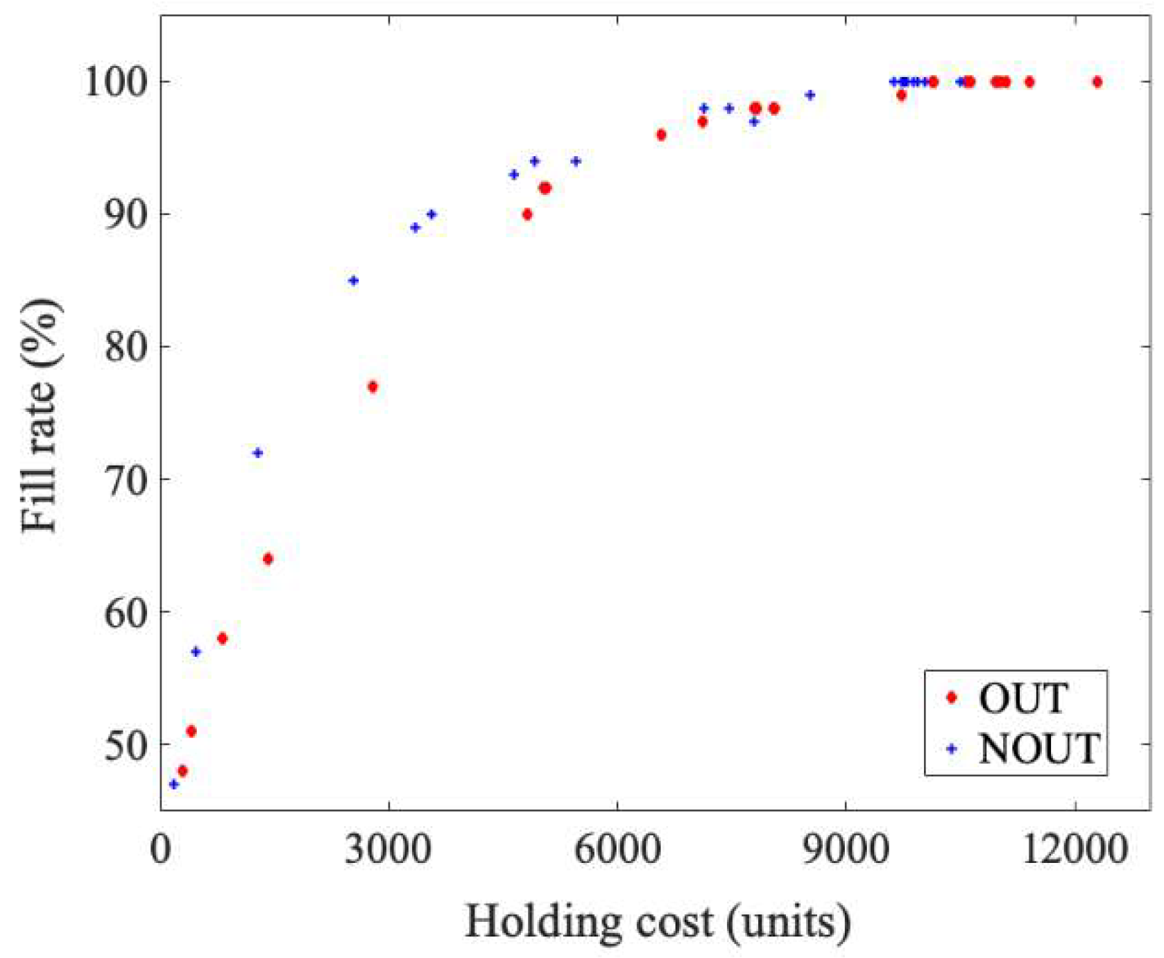
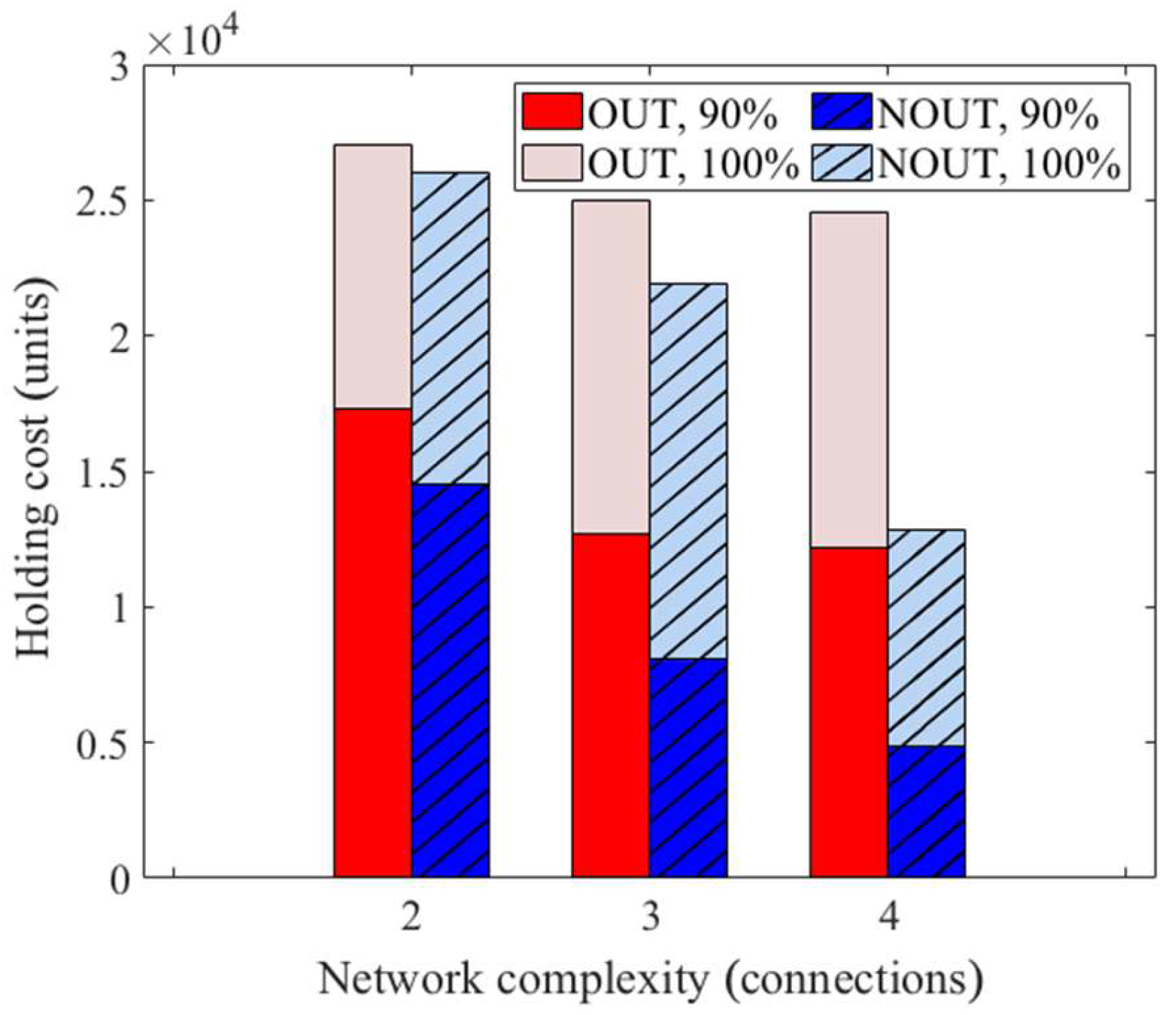
5.2.2. Large Network (N2)

Network N2 encompassed four external sources and ten controlled nodes. The considered interconnection structure is illustrated in Figure 9. The lead-time delays were randomly selected from the range 1–7. The holding cost from the initial, worst-case simulation performed for the maximum persistent demand amounted to 7.73 × 10⁵ units. The corresponding domain for the exhaustive search encompassed 1033 combinations, thus being infeasible for the common computing platforms. The comparison of the initial RSLs calculated for the controlled nodes using (15) and the optimal vector determined using CGA is visualized in Figure 10.
Figure 11 depicts the performance measures obtained for the considered network topology and Table 9 groups the numerical data. When compared with the small-network case discussed in the previous section, larger differences can be noticed between the investigated policies, which were all in favor of the centralized strategy NOUT. In the analyzed case of the network from Figure 9, the cost savings for a given fill rate fell in the range of 5–43%. The biggest savings in the case of the better, centralized, policy, for both the full and partial customer satisfaction, are marked in bold in Table 9.
These observations are quite general. As was investigated for different network sizes and structural complexities, the cost-related benefits of the NOUT policy relative to the standard one grew for larger and more intricate topologies. Figure 12 summarizes the policy performances under different fill rate requirements. The bars represent three different topologies, involving three, four, and five supply nodes connected to each controlled node, respectively. The stacked bars reflect the overall holding cost for full (100%) and high (90%) customer satisfaction levels. As expected, the holding costs decreased when relaxing the fill rate objective. The gain from using the centralized policy relative to the standard one grew for more complex topologies. Interestingly, the holding costs decreased for more involved connectivity structures. This was probably caused by an averaging effect, i.e., although encompassing more nodes and having a denser linkage structure, the topology became more regular with respect to the connection specifics, e.g., the mean lead-time delay for a given node.
Figure 13 presents the changes in the fitness function in the CGA search process. The same business objectives as for network N1, parametrized using γ = 1 and φ = 20, were considered. Despite having initially better effectiveness in the case of the OUT policy, ultimately, in line with the theoretical assumptions, the search for the best RSLs for the NOUT policy continued to progress beyond the level established for the OUT one and approached the optimal selection more closely.

6. Results Discussion and Conclusions

This study investigated the performance of CGAs with respect to the automatic parameter adjustment of inventory control strategies in logistic networks that have complex, mesh-type topologies. Two such strategies were examined: the classical OUT policy implemented in a distributed way and a centralized one that took into account the network connectivity structure. The analytical study, which was confirmed by the conducted numerical experiments, demonstrated that the centralized decision-making allowed one to lower the holding costs while maintaining the requested service level relative to the distributed approach.
The performed numerical studies confirmed that the CGA-based optimization was an effective tool for the optimization of logistic networks, even in the case of complex interconnection structures. It allowed one to reduce the computational time and effort (relative to the full-search approach), while yielding a near-optimal outcome. Moreover, the CGA-based optimization provided a considerable improvement over the typically applied MC approach in terms of accuracy and convergence time. Hence, it can be considered as a viable alternative to the traditional tuning procedures, especially in systems with irregular topologies. For the sake of clearer visualization, the reported numerical studies showed systems consisting of a relatively small number of nodes, i.e., a few, or a dozen. This scale may either reflect a small distribution network, e.g., a regional store network, or serve as a projection of an extended one (e.g., a continent divided into countries or a country divided into states). Strenuous tests of the CGA-based optimization of the interconnection structures involving hundreds or thousands of nodes is an area for further research. The analysis of the execution time indicated that such structures might require parallelization techniques to conduct the computations.
From the managerial perspective, the conducted research offered a few important insights. First, it was evidenced that in the considered class of systems, the application of a centralized OUT policy was economically more efficient than the distributed one, although it required a common view of the system. The greater the structural complexity, the bigger the economic profits that were gained in the centralized approach. The CGA-based optimization may be flexibly adapted according to diverse system requirements. The applied fitness function allows system managers to smoothly balance the optimization objectives, notably, the customer satisfaction vs. the operational costs, using just two numerical coefficients. In particular, a simultaneous increase of both coefficients enables achieving full customer satisfaction with maximum economic savings. Moreover, in the proposed framework, the objectives can be redefined, or replaced, without altering the computational scheme itself. The framework can also be customized to support other inventory control policies besides OUT, albeit with different search-space constraints and other fitness functions that balance the optimization goals would need to be specified.
There are a few directions in which the presented research could be extended. One may address the robustness issues, e.g., how to adjust the CGA for a yet more involved case of networks with uncertain, time-varying parameters and topologies (inaccurate inventory records, node failures, etc.). Furthermore, other evolutionary algorithms may be implemented and compared with the discussed CGA-based optimization with respect to the time and efficiency when seeking the optimal solution. Since in inventory management problems, one typically faces a number of conflicting goals, multi-objective optimization algorithms may also be considered.

Author Contributions

Conceptualization, P.I. and Ł.W.; methodology, P.I.; software, Ł.W.; validation, Ł.W.; formal analysis, P.I.; writing—original draft preparation, Ł.W.; writing—review and editing, P.I.; visualization, Ł.W.; supervision, P.I.; funding acquisition, Ł.W. All authors have read and agreed to the published version of the manuscript.

Funding

This research was funded by the Faculty of Technical Physics, Information Technology and Applied Mathematics, Lodz University of Technology, within the framework of the project entitled “Optimization of resource distribution process in complex logistic networks using genetic algorithms”.

Conflicts of Interest

The authors declare no conflict of interest.

References

  1. Ignaciuk, P.; Bartoszewicz, A. Linear-quadratic optimal control of periodic-review perishable inventory systems. IEEE Trans. Control Syst. Technol. 2012, 20, 1400–1407. [Google Scholar] [CrossRef]
  2. Shaban, A.; Shalaby, M.A.; Di Gravio, G.; Patriarca, R. Analysis of Variance Amplification and Service Level in a Supply Chain with Correlated Demand. Sustainability 2020, 12, 6470. [Google Scholar] [CrossRef]
  3. Ignaciuk, P. Discrete inventory control in systems with perishable goods—A time-delay system perspective. IET Control Theory A 2014, 8, 11–21. [Google Scholar] [CrossRef]
  4. Yuan, B.; He, L.; Gu, B.; Zhang, Y. The Evolutionary Game Theoretic Analysis for Emission Reduction and Promotion in Low-Carbon Supply Chains. Appl. Sci. 2018, 8, 1965. [Google Scholar] [CrossRef] [Green Version]
  5. Ignaciuk, P. Nonlinear inventory control with discrete sliding modes in systems with uncertain delay. IEEE Trans. Ind. Inform. 2014, 10, 559–568. [Google Scholar] [CrossRef]
  6. Chu, Y.; You, F.; Wassick, J.M.; Agarwal, A. Simulation-based optimization framework for multi-echelon inventory systems under uncertainty. Comput. Chem. Eng. 2015, 73, 1–16. [Google Scholar] [CrossRef]
  7. Patriarca, R.; Hu, T.; Costantino, F.; Di Gravio, G.; Tronci, M. A System-Approach for Recoverable Spare Parts Management Using the Discrete Weibull Distribution. Sustainability 2019, 11, 5180. [Google Scholar] [CrossRef] [Green Version]
  8. Cattani, K.D.; Jacobs, F.R.; Schoenfelder, J. Common inventory modeling assumptions that fall short: Arborescent networks, Poisson demand, and single-echelon approximations. J. Oper. Manag. 2011, 29, 488–499. [Google Scholar] [CrossRef]
  9. Papadopoulos, C.T.; Li, J.; O’Kelly, M.E.J. A classification and review of timed Markov models of manufacturing systems. Comput. Ind. Eng. 2019, 128, 219–244. [Google Scholar] [CrossRef]
  10. Ignaciuk, P.; Wieczorek, Ł. Optimization of mesh-type logistic networks for achieving max service rate under order-up-to inventory policy. Adv. Intell. Syst. 2018, 657, 118–127. [Google Scholar] [CrossRef]
  11. Min, H. Artificial intelligence in supply chain management: Theory and applications. Int. J. Logist. Appl. 2010, 13, 13–39. [Google Scholar] [CrossRef]
  12. Baryannis, G.; Validi, S.; Dani, S.; Antoniou, G. Supply chain risk management and artificial intelligence: State of the art and future research directions. Int. J. Prod. Res. 2018, 57, 2179–2202. [Google Scholar] [CrossRef]
  13. Ko, M.; Tiwari, A.; Mehnen, J. A review of soft computing applications in supply chain management. Appl. Soft Comput. 2010, 10, 661–674. [Google Scholar] [CrossRef] [Green Version]
  14. Knoll, D.; Prüglmeier, M.; Reinhart, G. Predicting future inbound logistics processes using machine learning. Proc. CIRP 2016, 52, 145–150. [Google Scholar] [CrossRef] [Green Version]
  15. González-Reséndiz, J.; Arredondo-Soto, K.C.; Realyvásquez-Vargas, A.; Híjar-Rivera, H.; Carrillo-Gutiérrez, T. Integrating Simulation-Based Optimization for Lean Logistics: A Case Study. Appl. Sci. 2018, 8, 2448. [Google Scholar] [CrossRef] [Green Version]
  16. Rivera-Gómez, H.; Montaño-Arango, O.; Corona-Armenta, J.R.; Garnica-González, J.; Ortega-Reyes, A.O.; Anaya-Fuentes, G.E. JIT Production Strategy and Maintenance for Quality Deteriorating Systems. Appl. Sci. 2019, 9, 1180. [Google Scholar] [CrossRef] [Green Version]
  17. Pourhejazy, P.; Kwon, O.K. The New Generation of Operations Research Methods in Supply Chain Optimization: A Review. Sustainability 2016, 8, 1033. [Google Scholar] [CrossRef] [Green Version]
  18. Simon, D. Evolutionary Optimization Algorithms; John Wiley & Sons: Hoboken, NJ, USA, 2013. [Google Scholar]
  19. Jauhar, S.K.; Pant, M. Genetic algorithms in supply chain management: A critical analysis of the literature. Sādhanā 2016, 41, 993–1017. [Google Scholar] [CrossRef] [Green Version]
  20. Lee, C.K.H. A review of applications of genetic algorithms in operations management. Eng. Appl. Artif. Intel. 2018, 76, 1–12. [Google Scholar] [CrossRef]
  21. Mihăiţă, A.S.; Dupont, L.; Camargo, M. Multi-objective traffic signal optimization using 3D mesoscopic simulation and evolutionary algorithms. Simul. Model. Pract. Theory 2018, 86, 120–138. [Google Scholar] [CrossRef]
  22. Axsäter, S. Inventory Control; Springer: New York, NJ, USA, 2015. [Google Scholar]
  23. Ignaciuk, P. Dynamic modeling and order-up-to inventory management in logistic networks with positive lead time. In Proceedings of the 2015 IEEE International Conference on Intelligent Computer Communication and Processing (ICCP), Cluj-Napoca, Romania, 3–5 September 2015; pp. 507–510. [Google Scholar] [CrossRef]
  24. Dominguez, R.; Cannella, S.; Framinan, J.M. On bullwhip-limiting strategies in divergent supply chain networks. Comput. Ind. Eng. 2014, 73, 85–95. [Google Scholar] [CrossRef]
  25. Wangphanich, P.; Kara, S.; Kayis, B. Analysis of the bullwhip effect in multi-product, multi-stage supply chain systems—A simulation approach. Int. J. Prod. Res. 2010, 48, 4501–4517. [Google Scholar] [CrossRef]
  26. Basten, R.J.I.; van Houtum, G.J. Near-optimal heuristics to set base stock levels in a two-echelon distribution network. Int. J. Prod. Econ. 2013, 143, 546–552. [Google Scholar] [CrossRef] [Green Version]
  27. Chang, K.H.; Lu, Y.S. Inventory management in a base-stock controlled serial production system with finite storage space. Math. Comput. Model. 2011, 54, 2750–2759. [Google Scholar] [CrossRef]
  28. Albrecht, M. Determining near optimal base-stock levels in two-stage general inventory systems. Eur. J. Oper. Res. 2013, 232, 342–349. [Google Scholar] [CrossRef]
  29. Wang, Q. A periodic-review inventory control policy for a two-level supply chain with multiple retailers and stochastic demand. Eur. J. Oper. Res. 2013, 230, 53–62. [Google Scholar] [CrossRef]
  30. Guerrero, W.J.; Yeung, T.G.; Guéret, C. Joint-optimization of inventory policies on a multi-product multi-echelon pharmaceutical system with batching and ordering constraints. Eur. J. Oper. Res. 2013, 231, 98–108. [Google Scholar] [CrossRef]
  31. Eruguz, A.S.; Jemai, Z.; Sahin, E.; Dallery, Y. Optimising reorder intervals and order-up-to levels in guaranteed service supply chains. Int. J. Prod. Res. 2014, 52, 149–164. [Google Scholar] [CrossRef] [Green Version]
  32. Avci, M.G.; Selim, H. A Multi-objective, simulation-based optimization framework for supply chains with premium freights. Expert. Syst. Appl. 2017, 67, 95–106. [Google Scholar] [CrossRef]
  33. Horng, S.C.; Lin, S.S. Ordinal optimization based metaheuristic algorithm for optimal inventory policy of assemble-to-order systems. Appl. Math. Model. 2017, 42, 43–57. [Google Scholar] [CrossRef]
  34. Feng, P.; Wu, F.; Fung, R.Y.K.; Jia, T.; Zong, W. The order and transshipment decisions in a two-location inventory system with demand forecast updates. Comput. Ind. Eng. 2019, 135, 53–66. [Google Scholar] [CrossRef]
  35. Dominguez, R.; Cannella, S.; Framinan, J.M. The impact of the supply chain structure on bullwhip effect. Appl. Math. Model. 2015, 39, 7309–7325. [Google Scholar] [CrossRef]
  36. Ignaciuk, P.; Bartoszewicz, A. Linear-quadratic optimal control strategy for periodic-review inventory systems. Automatica 2010, 46, 1982–1993. [Google Scholar] [CrossRef]
  37. Lim, J.; Norman, B.A.; Rajgopal, J. Redesign of vaccine distribution networks. Int. Trans. Oper. Res. 2019. [Google Scholar] [CrossRef]
  38. Grob, C. Inventory Management in Multi-Echelon Networks: On the Optimization of Reorder Points; Springer: Wiesbaden, Germany, 2019. [Google Scholar]
  39. Ignaciuk, P.; Wieczorek, Ł. Networked base-stock inventory control in complex distribution systems. Math. Probl. Eng. 2019, 2019, 3754367. [Google Scholar] [CrossRef] [Green Version]
  40. Ivanov, D. Simulation-based ripple effect modelling in the supply chain. Int. J. Prod. Res. 2016, 55, 2083–2101. [Google Scholar] [CrossRef]
  41. Song, W.; Xi, H.; Kang, D.; Zhang, J. An agent-based simulation system for multi-project scheduling under uncertainty. Simul. Model. Pract. Theory 2018, 86, 187–203. [Google Scholar] [CrossRef]
  42. Wang, Y.; Shi, Q. Improved dynamic PSO-Based algorithm for critical spare parts supply optimization under (T, S) inventory policy. IEEE Access 2019, 7, 153694–153709. [Google Scholar] [CrossRef]
  43. Koulouriotis, D.E.; Xanthopoulos, A.S.; Tourassis, V.D. Simulation optimisation of pull control policies for serial manufacturing lines and assembly manufacturing systems using genetic algorithms. Int. J. Prod. Res. 2010, 48, 2887–2912. [Google Scholar] [CrossRef] [Green Version]
  44. Paul, B.; Rajendran, C. Rationing mechanisms and inventory control-policy parameters for a divergent supply chain operating with lost sales and costs of review. Comput. Oper. Res. 2011, 38, 1117–1130. [Google Scholar] [CrossRef]
  45. Ambekar, S.; Kapoor, R. Optimization of inventory policies of food grain distribution stage in public distribution system. Benchmark Int. J. 2019, 26, 692–713. [Google Scholar] [CrossRef]
  46. Senoussi, A.; Dauzère-Pérès, S.; Brahimi, N.; Penz, B.; Mouss, N.K. Heuristics Based on Genetic Algorithms for the Capacitated Multi Vehicle Production Distribution Problem. Comput. Oper. Res. 2018, 96, 108–119. [Google Scholar] [CrossRef]
  47. Pal, A.; Kant, K. Smartporter: A Combined Perishable Food and People Transport Architecture in Smart Urban Areas. In Proceeding of the 2016 IEEE International Conference on Smart Computing (SMARTCOMP), St. Louis, MI, USA, 18–20 May 2016; pp. 1–8. [Google Scholar] [CrossRef]
  48. Murali, P.; Ordóñez, F.; Dessouky, M.M. Modeling strategies for effectively routing freight trains through complex networks. Transp. Res. Part C Emerg. Technol. 2016, 70, 197–213. [Google Scholar] [CrossRef]
  49. Deng, L.B.; He, Y.; Zeng, N.X.; Zeng, J.H. Optimal Design of Feeder-Bus Network with Split Delivery. J. Transp. Eng. Part A Syst. 2020, 146, 04019078. [Google Scholar] [CrossRef]
  50. Zhou, K.; He, S.; Song, R.; Guo, X.; Li, K. Optimization Model and Algorithm of Empty Pallets Dispatching under the Time-Space Network of Express Shipment. J. Adv. Transp. 2018, 2018, 1897936. [Google Scholar] [CrossRef]
  51. Zhou, Y.; Liu, J.; Zhang, Y.; Gan, X. A multi-objective evolutionary algorithm for multi-period dynamic emergency resource scheduling problems. Transp. Res. Part E Logist. Transp. Rev. 2017, 99, 77–95. [Google Scholar] [CrossRef]
  52. Haghi, M.; Ghomi, S.M.T.F.; Jolai, F. Developing a robust multi-objective model for pre/post disaster times under uncertainty in demand and resource. J. Clean. Prod. 2017, 154, 188–202. [Google Scholar] [CrossRef]
  53. Petrović, M.; Miljković, Z.; Jokić, A. A novel methodology for optimal single mobile robot scheduling using whale optimization algorithm. Appl. Soft Comput. 2019, 81, 105520. [Google Scholar] [CrossRef]
  54. Wang, Y.; Geng, X.; Zhang, F.; Ruan, J. An immune genetic algorithm for multi-echelon inventory cost control of IoT based supply chains. IEEE Access 2018, 6, 8547–8555. [Google Scholar] [CrossRef]
  55. Ignaciuk, P. State-space modeling and analysis of order-up-to goods distribution networks with variable demand and positive lead time. Adv. Intell. Syst. 2017, 524, 55–65. [Google Scholar] [CrossRef]
  56. Roberge, V.; Tarbouchi, M.; Labonte, G. Fast genetic algorithm path planner for fixed-wing military UAV Using GPU. IEEE Trans. Aerosp. Electron. Syst. 2018, 54, 2105–2117. [Google Scholar] [CrossRef]
Figure 1. Operational sequence at a controlled node.
Applsci 10 07851 g001
Figure 2. Genetic algorithm (GA) block diagram.
Applsci 10 07851 g002
Figure 3. Four-way tournament selection in a P-size population {S1, …, SP}: I—random selection of four individuals, II—selection of the best (most fit) individual.
Applsci 10 07851 g003
Figure 4. Two-point crossover operation.
Applsci 10 07851 g004
Figure 5. Fitness function improvements of the MC simulations vs. the CGA with fitness function coefficients equal (a) γ = 1, φ = 1; (b) γ = 1, φ = 10; (c) γ = 10, φ = 10.
Applsci 10 07851 g005
Figure 6. Goods distribution network N1.
Applsci 10 07851 g006
Figure 7. Fill rate vs. holding cost trade-off for network N1.
Applsci 10 07851 g007
Figure 8. Fitness function improvements.
Applsci 10 07851 g008
Figure 9. Goods distribution network N2.
Applsci 10 07851 g009
Figure 10. Initial and optimal reference stock levels (RSLs) for network N2.
Applsci 10 07851 g010
Figure 11. Fill rate vs. holding costs trade-off for network N2.
Applsci 10 07851 g011
Figure 12. Relation of holding cost with respect to the network complexity in terms of the policy used and the customer satisfaction.
Applsci 10 07851 g012
Figure 13. Fitness function improvements.
Applsci 10 07851 g013
Table 1. Mathematical preliminaries.
NotationDescription
(…)+The saturation function restricting the argument to non-negative values
t = 1, 2, …, TPeriod, where T is the planning horizon
ΘN = {1, 2, …, N}The set containing the controlled node indices, where N is their total number
ΘM = {1, 2, …, M}The set containing the external source indices, where M is their total number
αijNominal supplier fraction between nodes i and j, i.e., the part of the replenishment signals generated by node j that is requested from supplier i
αij(t)Supplier fraction between nodes i and j in period t
βijLead-time delay between nodes i and j, i.e., the time from placing the order to its delivery
BThe highest lead-time delay between any two nodes in the system
li(t)The on-hand stock level at node i in period t
di(t)The external demand imposed on node i in period t
si(t)The external demand satisfied by node i in period t
oi(t)The amount of goods to be ordered by node i at the end of period t from its suppliers
Ω i S ( t ) The quantity of goods in replenishment orders sent by node i to its neighbors in period t
Ω i R ( t ) The quantity of goods in replenishment orders received by node i from its suppliers in period t
l(t)The vector containing on-hand stock levels at the controlled nodes in period t
d(t)The vector containing the external demands imposed on the controlled nodes in period t
s(t)The vector containing the external demands satisfied by the controlled nodes in period t
o(t)The vector containing the replenishment signals generated by the controlled nodes in period t
Table 2. Optimization results for different population sizes.
Population SizeFitness Function ValueBest Fitness Value RatioSimulation Time (ms)
40.83350.936216,914
100.87780.985943,292
500.88230.9910479,072
1000.89041.0000583,971
Table 3. Optimization results for different selection methods.
Selection MethodFitness Function Value
Stochastic universal sampling0.4872
Roulette wheel selection0.7655
Tournament selection0.8831
Table 4. Optimization results for different crossover methods.
Crossover MethodFitness Function Value
None0.0288
Single-point crossover0.7853
Multipoint crossover0.8865
Uniform crossover0.8242
Table 5. Optimization results for different mutation probabilities.
Mutation ProbabilityFitness Function Value
00.3931
0.010.8706
0.050.8690
0.10.8709
0.150.8823
0.250.8800
0.50.8031
Table 6. Continuous genetic algorithm (CGA) parameters for logistic network optimization.
PhaseParameterSetting
InitializationPopulation size10 individuals
Stop criterion103–104 generations
Fitness function Ψ = ( 1     H C H C max ) γ F R φ ,
EvolutionSelectionFour-way tournament selection
CrossoverTwo-point crossover
Mutation15% mutation probability
Table 7. Detailed results of the Monte Carlo (MC) method vs. the CGA.
Number of NodesOptimization MethodFitness Function CoefficientsPerformance IndicatorsBest Fitness FunctionFitness Value Difference
γφHolding CostFill Rate
5MC11308694%0.846910980.0013
5CGA11304394%0.84820807
5MC1107715100%0.752422820.0097
5CGA1107412100%0.7621462
5MC10167673%0.586238150.0031
5CGA10166073%0.58932219
14MC11806894%0.900664720.0427
14CGA11907699%0.94339654
14MC11031,326100%0.837522430.1008
14CGA11011,892100%0.93832014
14MC101443888%0.697182330.0485
14CGA101359390%0.74566725
27MC1159,82899%0.928879450.0425
27CGA1118,21099%0.97139658
27MC110105,453100%0.891180560.0763
27CGA11031,488100%0.96750679
27MC10142,87396%0.610593530.2361
27CGA10113,08697%0.84669328
Table 8. Policy performance in network N1.
Fitness Function CoefficientsOrder-Up-To
(OUT) Policy
Networked OUT
(NOUT) Policy
γφHolding CostFill RateHolding CostFill Rate
11783198%852399%
1510,965100%10,496100%
12010,576100%9882100%
15011,092100%10,036100%
110011,407100%9947100%
51481490%334789%
55803698%779297%
52010,124100%9808100%
55010,160100%9721100%
510011,026100%9748100%
20181958%128072%
205507392%356490%
2020806098%746798%
205010,625100%9804100%
2010012,287100%9763100%
50141151%46857%
505278377%253285%
5020658596%492194%
5050780498%714298%
50100972899%9635100%
100129648%17647%
1005141464%128272%
10020502892%356090%
10050711197%464693%
100100780398%546394%
Table 9. Policy performance in network N2. The biggest savings for full and partial customer satisfaction are given in bold.
Fitness Function CoefficientsOUT PolicyNOUT Policy
γφHolding CostFill RateHolding CostFill Rate
1170,538100%54,07999%
1571,022100%67,596100%
12075,454100%61,101100%
15076,549100%63,390100%
110093,568100%62,277100%
5134,99990%24,97793%
5565,24699%55,36399%
52079,339100%57,843100%
55087,859100%60,545100%
510073,144100%67,893100%
20115,84068%10,45677%
20541,02393%23,46392%
202058,95898%49,28299%
205077,607100%56,14999%
2010086,818100%56,96999%
501653847%534963%
50527,57784%16,68686%
502042,40294%30,86395%
505062,47598%54,07899%
5010071,686100%53,31899%
1001313935%291552%
100513,59464%10,74678%
1002036,21790%26,94793%
1005053,07497%33,80196%
10010063,70499%56,342100%
Publisher’s Note: MDPI stays neutral with regard to jurisdictional claims in published maps and institutional affiliations.

