Abstract
Displacement predictions are essential to landslide early warning systems establishment. Most existing prediction methods are focused on finding an individual model that provides a better result. However, the limitation of generalization that is inherent in all models makes it difficult for an individual model to predict different cases accurately. In this study, a novel coupled method was proposed, combining the long short-term memory (LSTM) neural networks and support vector regression (SVR) algorithm with optimal weight. The Shengjibao landslide in the Three Gorges Reservoir area was taken as a case study. At first, the moving average method was used to decompose the cumulative displacement into two components: trend and periodic terms. Single-factor models based on LSTM neural networks and SVR algorithms were used to predict the trend terms of displacement, respectively. Multi-factors LSTM and SVR models were used to predict the periodic terms of displacement. Precipitation, reservoir water level, and previous displacement are considered as the candidate factors for inputs in the models. Additionally, ensemble models based on the SVR algorithm are used to predict the optimal weight to combine the results of the LSTM and SVR models. The results show that the LSTM models display better performance than SVR models; the ensemble model with optimal weight outperforms other models. The prediction accuracy can be further improved by also considering results from multiple models.
1. Introduction
Since the impoundment of the Three Gorges Reservoir area (TGRA) in June 2003, many new landslides have occurred and some existing landslides have been reactive. The Shanshucao landslide took place on 2 September 2014, interrupting the power supply for the town and damaged around m2 area of orange planting [1]. The Honyanzi landslide took place on 24 June 2015, initiating a reservoir tsunami that resulted in two deaths and significant damage to shipping facilities [2]. As an essential component for landslide early warning systems, displacement predictions become ever more important in the TGRA.
In general, landslide displacement predictions involve the following steps: (i) the decomposition of total displacement, (ii) the selection of candidate factors, (iii) the establishment of predicting models, and (iv) the evaluation of prediction results. For the decomposition of total displacement (step i), the moving average method (MAM) [3], the empirical mode decomposition [4], the wavelet analysis [5,6], and the variational mode decomposition [7] have been proposed to obtain sub-sequences of total displacement. The obtained sub-sequences are usually defined as trend terms and periodic terms. The trend term of the original total displacement represents the component mainly caused by the state factors and the periodic term represents the component mainly caused by the influence factors. For the selection of input factors (step ii), the mutual information, the Pearson cross-correlation coefficient [4], and the grey correlation analysis method (GCAM) [8,9] have been used. In the TGRA, the landslide deformation is the consequence of the state and the influence factors, and these controlling factors are very diverse [10,11,12]. Thus, it is necessary to select factors before establishing models.
Since Saito [13] proposed the empirical formula for landslide prediction, many approaches to landslide displacement prediction have been developed [14], including those based on creep theory, statistical theory, time-series analysis, and artificial intelligence methods [15,16]. For artificial intelligence methods that have been applied in landslide displacement, the Gaussian process model [17], the neural network model [18,19,20], the Support Vector Machine (SVM) model [9,21,22], the Extreme Learning Machine (ELM) model [8,23,24], and the LSTM model [4,25] have become popular. Moreover, these approaches can also be divided into two categories which are univariate forecasting methods and multivariate forecasting methods. Univariate forecasting methods only consider previous displacement, while the multivariate forecasting methods consider triggering factor as well.
The current studies mainly focus on choosing single prediction models from the numerous artificial intelligence methods. Since some models many be only suitable for specific landslide, a specific type of landslides, or a set of landslides with specific local geological conditions, periods, and variations, it is necessary to study how to accurately and comprehensively different models predict landslides by considering advantages from different models [15,16]. Moreover, the linear combination is perhaps most well developed and mature [26]. Therefore, this study mainly focuses on an Ensemble model with the weight coefficients based on linear combination theory.
In this study, the accumulated displacements of the selected monitoring points on the Shengjibao landslide were decomposed into trend term and periodic term using the MAM. The trend terms were predicted using the univariate forecasting methods based on the LSTM and SVR algorithm, respectively. The periodic terms were predicted by the multivariate forecasting methods based on the LSTM and SVR algorithm with analyzing the relationship between landslide displacement and the triggering factors separately. The predictive total displacements of each model were obtained by adding their predictive trend and periodic terms. The final total predicting displacements were obtained by adding the predictive total displacements of both models with the weight coefficients obtained from the prediction of the optimal weight.
2. Methodology
2.1. Decomposition of the Displacement Time Series into Trend and Periodic Terms
Landslide displacement was modeled using two components: a trend component and a periodic component [3,27]. In the long-term, the deformation trend is controlled by internal geological conditions, such as lithology, geological structure, and progressive weathering. The short-term deformation in the TGRA is influenced by two main external triggering factors: rainfall and reservoir water level. The short-term displacement represents the periodic component in the model [25]. The accumulated displacement time series can be decomposed as follows:
where is the time step, is the accumulated displacement, is the trend term, and is the periodic term.
2.2. Moving Average Methods
The decomposition of the trend and periodic terms forms the basis of the model. If the period of the time series and influencing factors can be determined accurately, the fluctuation can be smoothed by the moving average method, and the trend term of the displacement can be extracted. The function of the single moving average method is shown as follows:
where is the trend term of the displacement at the time step , is the accumulative displacement of the landslide at the time step , is the moving average cycle. Considering the scheduling cycle of the TGRA, the moving average cycle was selected as 12 months [21].
2.3. Long Short-Term Memory Neural Networks
Recurrent neural networks (RNNs) (Figure 1) have been successfully applied to a variety of problems, such as speech recognition, language modeling, translation, and image captioning [28,29]. RNNs can utilize historical information and apply it to the current output, which allows for feedback in the networks [30]. The recurrent connections in the RNN implement passing information from one step of the network (time step ) to the next one (time step ). For a given input sequence , the hidden state vector sequence is , and the output sequence is . The output sequence y can be obtained by iterating the following equations from time to :
where and are the input and output at time step ; and are the hidden states at time step t and , respectively; is the prediction period; is the weight matrix between input and hidden vectors; represents the weight matrix between different time steps of the hidden vectors; represents the weight matrix that connects the hidden information to the output vectors; and are the corresponding bias vectors of and , respectively; and is the nonlinear activation function for hidden nodes.
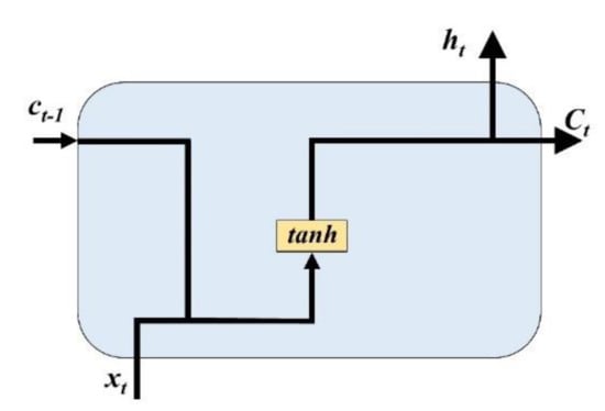
Figure 1.
Standard recurrent neural network (RNN) module contains a single layer.
However, in practice, RNNs are not capable of handling a problem as long-term dependencies because of the vanishing gradient or exploding gradient problems [31]. The LSTM neural networks are a special type of RNN, which are capable of learning long-term dependencies [32]. LSTMs replace every single unit in an RNN with a memory block (Figure 2). There are three types of gate functions in this memory block [33]. The input gates control the flow of input activations into the memory cell, and the output gates control the output flow into other cells or as the final results [34]. The forget gate controls whether the value from the previous moment is forgotten or remembered. The combination of the three types of gates controls the output state. The key difference between RNN and LSTM lies in the formulation of the hidden vector (). The hidden vector () in LSTM neural network can be obtained as follows:
where , , , and are the values of the input gate, the forget gate, the output gate, and the memory cell in the memory block; , , , and are their corresponding bias values; is the sigmoid function; represents the weights between input nodes and hidden nodes; represents the weights between hidden nodes and memory cell; represents the weights that connect memory cell to output nodes. The output can then be obtained by Equation (2). The output sequence will be obtained by iterating Equations (2) to (7) from times to .
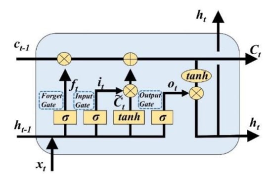
Figure 2.
Long short-term memory (LSTM) module contains four interacting layers.
2.4. Support Vector Regression
The support vector regression (SVR) model was proposed by Vapnik et al. in 1995 and has been widely used in nonlinear problem solving [35,36]. In SVR models, sample data are divided into a fitting sample and predicting sample. The fitting sample is then mapped to a high-dimensional feature space. The best fitting effect is obtained in the space of the optimal decision function model and the validation sample is used to validate the analytical model results. The regression function for SVR is:
where is the weight vector, is a nonlinear mapping from the input space to the output space, is bias. Transforming the estimation function into a function minimization problem by the insensitive loss function:
The constraint conditions are as follows:
where is the penalty factor; and are relaxation factors. The Lagrange multiplier is introduced at last, and converted into an equivalent dual problem based on the Wolf duality theory:
The constraint conditions are expressed in Equation (10):
where . The SVR prediction model can be obtained by quadratic programming:
where is the kernel function of SVR.
Linear kernel, polynomial kernel, radial basis kernel function (RBF), and sigmoid function [37] are four commonly used kernel functions for SVR algorithm. With a wide convergence domain, the RBF is widely used [21,38,39]. Therefore, the RBF is adopted as the kernel function for the SVR model in this paper.
2.5. Ensemble Model
We used ensemble models to reduce the instability of a single prediction model. The core idea of ensemble model is to assign different weight coefficients to the predictive results of different predicting models, to extract effective information from each model system, utilize the forecasting results of each model synthetically, disperse forecasting risks and errors, and improve the accuracy and reliability of predicting [15].
The displacement forecasts based on the LSTM model and the SVR model at the time step were and , the total displacement forecast of the ensemble algorithm was , the original displacement in the validation dataset at the time step was .
where is the dynamic weight coefficient obtained from the prediction of optimal weight.
2.6. Reliability Evaluation of the Model
After tuning the hyperparameters of the LSTM and SVR models with the fitting datasets, the training datasets and optimal hyperparameters were adopted to train the LSTM models and SVR models. To verify the prediction accuracy of the LSTM models, SVR models and the ensemble models, the root mean square error (RMSE) (Equation (13)) and mean absolute percentage error (MAPE) (Equation (14)) were calculated. The overall process is shown in Figure 3.
where is the measured value; is the predicted value; is the number of predicted values.
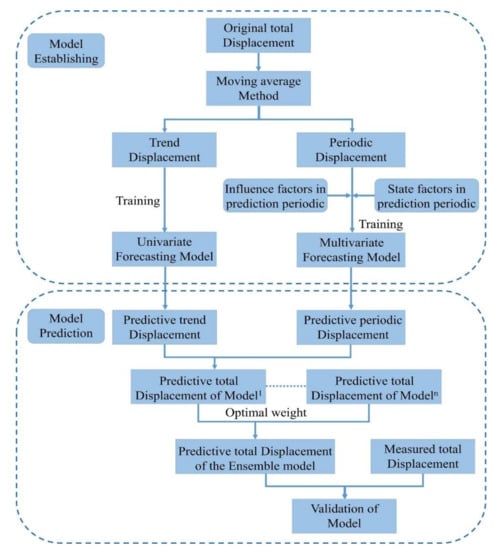
Figure 3.
Flowchart of the proposed predictive model.
3. Study Site
3.1. Shengjibao Landslide
The Shengjibao landslide is located on the South Bank of the Yangtze River in Fengjie County (Figure 4). The Yangtze River flows through the front of the landslide area from S72W. The overall landform type of the landslide is structure-erosion and denudation low-mountain valley. The Yangtze River Valley extends eastward in this section. The width of the river in this area is 350–400 m; the valley is V-shaped with asymmetrical banks. The topographic slope of the northern bank is steep, generally 30–50 degrees. The southern bank is a consequent slope with an overall slope of 15–20 degrees. The slope surface is ladder-like and gullies on the slope are well-developed. The slope gradient at the bottom of the gully is similar to that on the slope surface. The front elevation of the Shengjibao landslide is 81–85 m, the escarpment elevation is 370 m. The gradient range is 15–20 degrees and the longitudinal length is 1500 m. The lateral average width is about 1160 m, the average thickness is 25 m, the total area of landslide is about 2.45 km2, and the total volume of the landslide is 3998 × 104 m3.
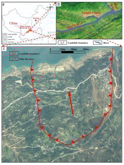
Figure 4.
(a) Location of the Three Gorges Reservoir Area (TGRA) in China; (b) location of the Shengjibao landslide; (c) overall view of the Shengjibao landslide (satellite image from Google Earth).
3.2. Landslide Activity
The initial monitoring network of Shengjibao landslide was established in March 2007, which includes 16 horizontal displacement monitoring points (Figure 5). In May 2007, Shengjibao landslide began to deform after the first 156 m impoundment of the TGRA, which was affected by the drop of the reservoir water level and seasonal rainfall. Movement has been small-scale controlled by the topography and generally occurred in the loose soil of the surface layer.
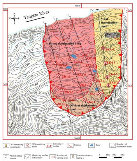
Figure 5.
Monitoring arrangement in the Shengjibao landslide and displacement blocks.
The main manifestations are the deformation of some houses, discontinuous cracks on the ground, and ground tilt (Figure 6). The main slide direction of the landslide is 348 degrees and a typical schematic geological cross-section is shown in Figure 7. Based on data collected from March 2007 to December 2015 (Figure 8), four stages of surface displacement along the II-II’ profile could be identified (Table 1).
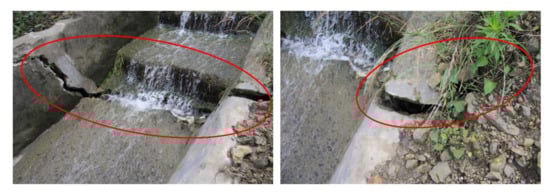
Figure 6.
Deformation indications on the Shengjibao landslide.
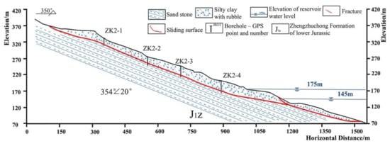
Figure 7.
A Schematic geological cross-section II-II’ of the Shengjibao landslide.
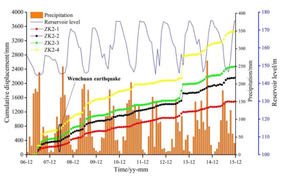
Figure 8.
Rainfall, reservoir water level, and cumulative displacement monitoring data from the landslide area.

Table 1.
Deformation stages of the Shengjibao landslide.
According to the reservoir water level data, the Shengjibao landslide did not show an obvious displacement during the period from March 2007 to May 2007, which was the discharge period after the first 156 m experimental impoundment of the TGRA. The operation period of the low water level (145 m) in the flood season of the reservoir was from 1 June 2007 to 20 September 2007. Reservoir water level fluctuations were not significant during this period. However, landslide deformation, characterized by increased displacement of the monitoring points, was obvious during this period, with rainfall being the dominant control on landslide deformation. From October 2007 to January, 2008, the reservoir water level rose again to 156 m. But the displacement of landslide monitoring points did not change significantly during this period.
The displacement data showed a sharp increase in surface displacement in August and September 2013 (Figure 8). However, a similar pattern was not detected in August and September 2014, despite comparable rainfall levels. According to the precipitation data showed in Figure 9, there was a rainfall pattern that lasted for 15 days during the period in 2013, and a rainfall pattern only lasted for 9 days in 2014. This indicates that under the same fluctuation conditions of reservoir water level, a longer duration of rainfall has a more important influence on landslide deformation.
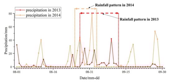
Figure 9.
Precipitation from August to September in 2013 and 2014.
4. Prediction Process
4.1. Point Selection and Data Processing
As shown in Figure 5, there were three types of deformation zones on the Shengjibao landslide: strong deformation zone, obvious deformation zone, and weak deformation zone. We selected ZK2-1 and ZK2-3 from the obvious deformation zone and the strong deformation zone, respectively, to represent two types of deformation points on the Shengjibao landslide.
Eighty-four measured values from January 2009 to December 2015 were adopted for establishing predictive models from the GPS monitoring points as ZK2-1 and ZK2-3. First, the adopted values were decomposed with MAM into trend terms and periodic terms. After decomposition, as suggested by Yang [25], 72 values were set as the fitting dataset, 48 values were set as the training dataset to fit the models, and 24 values were set as validation dataset to tune the hyperparameters of the models. Twelve values were set as predicting dataset to evaluate the capability of the models (Figure 10).
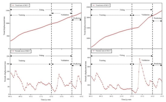
Figure 10.
Trend and Periodic terms of ZK2-1 and ZK2-3 measurements in Shengjibao landslide.
4.2. Factors Selection
Selecting the proper triggering factors is essential to guarantee the accuracy of a prediction. First, the candidate factors were determined with landslide deformation characteristics. Since displacement rates mainly increased during the rainy season and reservoir water level fluctuation stages (Figure 11), rainfall and reservoir water level were considered the main triggering factors that caused the deformation of the Shengjibao landslide. Additionally, the Wenchuan earthquake that occurred in May 2008 had an insignificant impact on the pattern of the landslide displacement according to the monitoring records shown in Figure 8 and Figure 11. Thus, the events of the earthquake were not considered as candidate factors for prediction. As the values of GPS monitoring data were obtained at the end of each month, the candidate factors should include the precipitation during the current month, the precipitation during the past two months, the average reservoir level during the current month, and the change of the reservoir level during the current month, the change of the reservoir level during the past two months. These candidate factors were considered as , , , , .
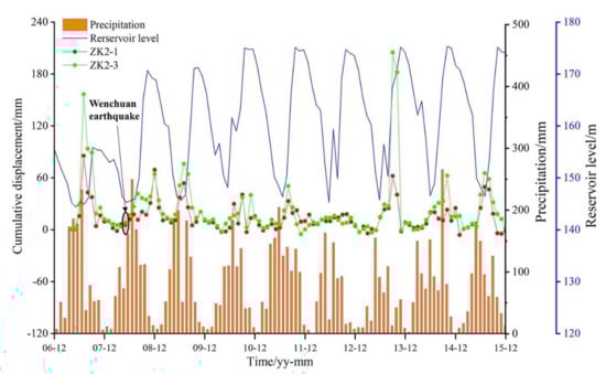
Figure 11.
Rainfall, reservoir water level, and displacement increment of ZK2-1 and ZK2-3.
Slopes in different evolutionary states may respond differently to the same external trigger factors. When the slope is stable, even strong influence factors are usually not enough to cause large deformation. In contrast, if a slope is marginally stable or even unstable, the slightest increase in external “loads” may cause disequilibrium and large deformation [40]. Therefore, the state factors were also considered as input values. The candidate factors should include the change of the displacement during the last month, during the last two months, during the last three months, and the average displacement during the last 12 months (annual displacement rate). These candidate factors were considered as , , , .
A resolution coefficient of 0.5 was obtained using the GCAM. The relational degrees between the periodic term and the candidate factors are shown in Table 2. The candidate factors are closely related to the periodic term, , suggesting that the parameters were properly selected [41].
Table 2.
Relation degree between the periodic terms and the candidate factors.
4.3. Normalization and Inverse Normalization
LSTM is a type of Deep Learning Algorithms, while SVR is a type of Instance-Based Algorithm. Additionally, they are all Machine Learning (ML) Algorithms, while for ML Algorithms, normalization makes it easier to find optimal parameters and reduces the chances of getting stuck in local optimal [42,43]. To maximally preserve the distributions of the dataset, each triggering factor is normalized to [−1, 1] using linear normalization.
As stated in Section 4.1, the whole fitting datasets were assumed to be known, and the predicting datasets were considered unknown. To prevent information leakage, maximum and minimum values of inputs and outputs for normalization and inverse normalization were obtained from the fitting datasets, respectively.
where is the normalized value, is the original value, is the maximum value of the samples, and is the minimum value of the samples.
4.4. Parameters of LSTMs and SVRs
Keras framework [44] was used to establish LSTM models, while TensorFlow was used as the back end, and Python language was adopted to write the codes. As a time series forecasting experiment, hyperparameters of LSTM models were tuned with the Grid Search (GS) method [44]. Its process can be described as follows: plausible values for each parameter are combined, and then all the combination values are used in the training process of the model. The performance metric of each combination is typically measured by validation on the validation dataset. When all the parameter combinations have been tried, an optimal parameter combination with the best performances is returned automatically.
For LSTM models establishment, batch-size, and numbers of layers of LSTM models were determined with the GS method successively. In GS processing, the gird range of batch-size is [1, 20] with a grid step of 1, the gird range of layers is [2,8] with a grid step of 1. The optimal epochs were obtained with an early-stopping set during the algorithmic process, and the patience of early-stopping was set as 20 which means the algorithmic process will stop when the result has no improvement within 20 steps.
The SVR models were also operated in the Python language environment. The GS method was used to search for the optimal parameters of the SVR model. As stated in Section 2.4, the RBF was adopted as kernel function for the SVR model. The values of gamma (the kernel coefficient for RBF) and the values of (the penalty parameter) were determined with GS. In GS processing, the search range of gamma is [0.0075, 1] with a grid step of 0.0075, the search range of C is [1, 20] with a grid step of 1. The best parameters are shown in Table 3.
Table 3.
Optimal hyperparameters of LSTMs and support vector regressions (SVRs) used for the dataset.
5. Results
5.1. LSTM Models and SVR Models
Figure 12, Table 4 and Table 5 present the comparison between measured and predicted displacement of ZK2-1 and ZK2-3 using LSTM and SVR models. For ZK2-1, the values of RMSE and MAPE with the LSTM model were 13.79 mm and 0.74%, while the accuracy factors of the SVR model were 15.12 mm and 0.74%. For ZK2-3, the values of RMSE and MAPE with the LSTM model were 12.74 mm and 0.43%, while the accuracy factors of the SVR model were 15.43 mm and 0.60%.
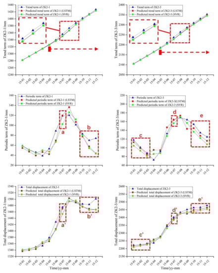
Figure 12.
The curves of the relationship between observed and predicted displacement.
Table 4.
Accuracy of the predicted displacement with the LSTM and SVR models of ZK2-1.
Table 5.
Accuracy of the predicted displacement with the LSTM and SVR models of ZK2-3.
In trend terms, the values of RMSE with the LSTM model and SVR model in ZK2-1 were 3.38 and 3.17 mm, and the values of RMSE with LSTM model and SVR model in ZK2-3were 5.23 and 6.26 mm. In periodic terms, the values of RMSE with the LSTM model and SVR model in ZK2-1 were 12.95 and 13.63 mm, and the values of RMSE with the LSTM model and SVR model in ZK2-3 were 10.92 and 10.62 mm (Table 6).
Table 6.
Accuracy of the prediction in trend term and periodic term of ZK2-1 and ZK2-3.
The LSTM models and SVR models both had worse performances after May 2015. LSTM models had significantly better performance in step a, period c, step d, and period e than SVR models. The performances of the models in step a, period b, period c, step d, and period e in the periodic terms were reflected in the total displacement (Figure 12).
5.2. Ensemble Models
Eight models were established by tuning hyperparameters and training for prediction. In this section, the whole datasets with 84 time-steps of ZK2-1 and ZK2-3 were applied to make predictions with the LSTM models and SVR models. The total prediction displacements of ZK2-1 and ZK2-3 from January 2009 to December 2015 with LSTM models and SVR models can be obtained with this process. An optimal weight can be obtained with setting the original total displacements as in Equation (12).
The optimal weights were set as outputs, and all the inputs that show in Table 2, the obtained total prediction displacements with LSTM models, the obtained total prediction displacements with SVR models, and the difference between these two total prediction displacements were set as candidate input factors. The latter 3 new candidate factors were considered as , , .
An SVR model using the GS method was adopted to predict the optimal weight for an ensemble model. As stated in Section 4.1, 84 measured values were adopted for finding a better model between LSTMs and SVRs. For the ensemble model runs, 72 time-steps were set as the fitting dataset, 48 time-steps were set as a training dataset to fit the models, and 24 time-steps were set as validation dataset to tune the hyperparameters of the SVR models and to determine the optimal inputs (Table 7). Twelve time-steps were set to evaluate the models. The optimal weights were set as 1 when the predicting values were more than 1, and were set as 0 when the predicting values were less than 0.
Table 7.
Optimal hyperparameters and inputs of SVRs used for optimal weight prediction.
Figure 13, Table 8 and Table 9 present the comparison between measured and predicted displacement of ZK2-1 and ZK2-3 using LSTM, SVR, and ensemble models. For the total displacement term of ZK2-1, the values of RMSE and MAPE with the Ensemble model were 13.76 mm and 0.73%, while the accuracy factors of the LSTM model were 13.79 mm and 0.74%, and the accuracy factors of the SVR model were 15.12 mm and 0.74%.
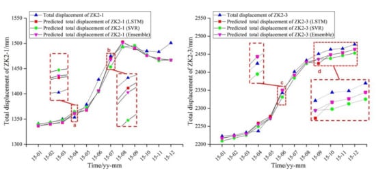
Figure 13.
The curves of the relationship between observed and predicted displacement.
Table 8.
Accuracy of the predicted displacement with the Ensemble models of ZK2-1.
Table 9.
Accuracy of the predicted displacement with the LSTM and SVR models of ZK2-3.
For the total displacement term of ZK2-3, the values of RMSE and MAPE with the Ensemble model were 10.70 mm and 0.40%, while the accuracy factors of the LSTM model were 12.74 mm and 0.43%, and the accuracy factors of the SVR model were 15.43 mm and 0.60%.
The total displacements predicted by the Ensemble model were in better agreement with the measured values than those with the LSTM or SVR models. As shown in Figure 13, in point a, point b, point c, and period d, the results of the Ensemble models tend to be closer to the results of original values than at least one of the LSTM or SVR models. This suggests that when the results of the LSTM and SVR models are different, the Ensemble model gives more weight to the results of the model that are closer to the real values. As shown in Table 8, in 12 predicted points of ZK2-1, 7 of them were had lower values of absolute error than the LSTM model, 5 of them had lower values of absolute error than the SVR model. As shown in Table 9, in 12 predicted points of ZK2-3, 2 of them were had lower values of absolute error than LSTM model, 10 of them had lower values of absolute error than SVR model.
6. Discussion
Considering predicting total displacement, the LSTM models showed a more satisfactory performance than the SVR models in ZK2-1 and ZK2-3, respectively, and the proposed Ensemble models yield relatively better results (Table 8 and Table 9). In predicting trend terms, the LSTM models showed better performance than SVR models in ZK2-3 and worse performance in ZK2-1. In predicting periodic terms, the LSTM models showed better performance than SVR models in ZK2-1 and worse performance in ZK2-3. This suggests that the accuracy of the total displacement prediction does not depend in the case of the Shengjibao landslide on the accuracy of only one sub-sequence.
Meanwhile, the generalization ability of the models directly affects the performance of the test dataset. The models established based on the performance on the validation dataset do not always perform as expected on the predicting dataset. As shown in Table 6 and Table 10, the LSTM models did not achieve the expected performance in predicting the trend term of ZK2-1 or the periodic term of ZK2-3, while the SVR model did not achieve the expected performance in predicting the trend term of ZK2-3.
Table 10.
Accuracy of the prediction in trend term and periodic term of ZK2-1 and ZK2-3.
There have been few reports on the research of decomposing the original landslide displacement into trend term, periodic term, and stochastic term [7,9] up to now. The stochastic displacement is caused by some random factors such as wind load and vehicle load. In decomposing original displacement, we chose to ignore the stochastic term. One should consider means to develop optimal models for predicting the stochastic displacement in the future. Additionally, the stability of the location of the GPS monitoring control point is the key controlling factors of the reliability of the monitoring data. Thus, the evaluation of the stability of the GPS monitoring control point is an important content that cannot be ignored in the processing of displacement observation data.
As stated in Section 3.2, there is a sharp increase in the displacement rates in August and September 2013. Although the proposed method achieved good results in this study, if factors as the precipitation or water level suddenly change, or an unusual rainfall pattern occurs, the error in point-based displacement predictions will inevitably increase. Thus, solving this problem becomes highly necessary [9]. As the Shengjibao landslide is a wading landslide in the TGRA, the factors considered including precipitation, water level and displacement. One should, in the future, consider means to develop prediction approaches for landslides with different triggering factors. There are three types of deformation zones divided on Shengjibao landslide. Any single point cannot represent the displacement characteristics of the entire landslide. To differentiate spatial zones of comparably the deformation characteristics and select the monitoring data of representative points are within these zones are vital preparatory steps for displacement prediction studies.
According to the existed research on the application of ML techniques to landslide displacement prediction up to now, many hybrid models were established for prediction. However, this research mainly focus on the hybrid models of the coupled single ML models and models used to obtain optimal hyperparameters for these proposed single ML models. In this study, an ensemble model of the coupled LSTM and SVR algorithm with the weight coefficients based on linear combination theory was established for prediction, and the ensemble model performed well. Meanwhile, many approaches to landslide susceptibility mapping and landslide risk analysis have been developed [45,46], including those based on artificial neural network [47,48], support vector machine [49], alternative decision tree [36]. In order to achieve an accurate result in landslide susceptibility mapping and landslide risk analysis, it is necessary to research more advanced ML algorithms. Thus, the novel method proposed in this paper is recommended for conducting landslide susceptibility mapping, landslide risk analysis, and other fields.
7. Conclusions
The monitoring data are fundamental for establishing landslide displacement prediction models, and the results of prediction are significant for landslide early warning. In this study, the Shengjibao landslide in the TRGA was taken as an example. Based on the monitoring data, the response relationship between landslide displacement and factors is analyzed, an ensemble model of the coupled LSTM and SVR algorithm with the weight coefficients based on linear combination theory was established. The dynamic model based on the deep learning algorithm of LSTM and the static SVR model were also used to predict landslide displacement for comparison. The main conclusions are as follows: (1) Under the same fluctuation conditions of reservoir water level, a longer duration of rainfall has a more important influence on landslide deformation; (2) Overall, the LSTM models perform better than the SVR models, but the results of LSTM models are not closer to the original value than the results of SVR models at every time step in predicting dataset; (3) The proposed Ensemble model integrated both the advantages of LSTM and SVR algorithms, where the Ensemble model has higher prediction performance than both of LSTM and SVR models. In general, by combing the advantages of different ML algorithms, the ensemble model proposed in this paper can effectively construct the response relationship between landslide displacement and factors.
Overall, the proposed method, which applies time series analysis, LSTM and SVR, can achieve accurate predictions in case of slow and the step-like deformation periods. This method of establishing an Ensemble model has the potential for application to predict landslide displacement in the TGRA and other landslide-prone regions.
Author Contributions
Writing—original draft preparation, H.J.; writing—review and editing, H.J., Y.L., C.Z., H.H., T.G., and K.Y.; supervision, K.Y. All authors have read and agreed to the published version of the manuscript.
Funding
This research was funded by the National Key R&D Program of China (No.292 2018YFC0809400).
Acknowledgments
We greatly appreciate the careful reviews and thoughtful suggestions by reviewers. The authors wish to thank Katrin Sattler and William Ries for their assistance in language improvement, and Xiaojing Chu for her technical support. The first author would like to thank the China Scholarship Council for funding his research at the University of Vienna, Austria.
Conflicts of Interest
The authors declare no conflict of interest.
References
- Xu, G.L.; Li, W.N.; Yu, Z.; Ma, X.H.; Yu, Z.Z. The 2 September 2014 Shanshucao landslide, Three Gorges Reservoir, China. Landslides 2015, 12, 1169–1178. [Google Scholar] [CrossRef]
- Xiao, L.; Wang, J.; Ward, S.N.; Chen, L. Numerical modeling of the June 24, 2015, Hongyanzi landslide generated impulse waves in Three Gorges Reservoir, China. Landslides 2018, 15, 2385–2398. [Google Scholar] [CrossRef]
- Du, J.; Yin, K.; Lacasse, S. Displacement prediction in colluvial landslides, Three Gorges Reservoir, China. Landslides 2013, 10, 203–218. [Google Scholar] [CrossRef]
- Xu, S.; Niu, R. Displacement prediction of Baijiabao landslide based on empirical mode decomposition and long short-term memory neural network in Three Gorges area, China. Comput. Geosci. 2018, 111, 87–96. [Google Scholar] [CrossRef]
- Huang, F.; Yin, K.; Zhang, G.; Gui, L.; Yang, B.; Liu, L. Landslide displacement prediction using discrete wavelet transform and extreme learning machine based on chaos theory. Environ. Earth Sci. 2016, 75. [Google Scholar] [CrossRef]
- Zhou, C.; Yin, K.; Cao, Y.; Ahmed, B.; Fu, X. A novel method for landslide displacement prediction by integrating advanced computational intelligence algorithms. Sci. Rep. 2018, 8, 7287. [Google Scholar] [CrossRef]
- Guo, Z.; Chen, L.; Gui, L.; Du, J.; Yin, K.; Do, H.M. Landslide displacement prediction based on variational mode decomposition and WA-GWO-BP model. Landslides 2019, 17, 567–583. [Google Scholar] [CrossRef]
- Cao, Y.; Yin, K.; Alexander, D.E.; Zhou, C. Using an extreme learning machine to predict the displacement of step-like landslides in relation to controlling factors. Landslides 2016, 13, 725–736. [Google Scholar] [CrossRef]
- Miao, F.; Wu, Y.; Xie, Y.; Li, Y. Prediction of landslide displacement with step-like behavior based on multialgorithm optimization and a support vector regression model. Landslides 2018, 15, 475–488. [Google Scholar] [CrossRef]
- Bernardie, S.; Desramaut, N.; Malet, J.P.; Gourlay, M.; Grandjean, G. Prediction of changes in landslide rates induced by rainfall. Landslides 2015, 12, 481–494. [Google Scholar] [CrossRef]
- Keefer, D.K.; Wilson, R.C.; Mark, R.K.; Brabb, E.E.; Brown, W.M.; Ellen, S.D.; Harp, E.L.; Wieczorek, G.F.; Alger, C.S.; Zatkin, R.S. Real-time landslide warning during heavy rainfall. Science 1987, 238, 921–925. [Google Scholar] [CrossRef]
- Oh, S.; Lu, N. Slope stability analysis under unsaturated conditions: Case studies of rainfall-induced failure of cut slopes. Eng. Geol. 2015, 184, 96–103. [Google Scholar] [CrossRef]
- Saito, M. Forecasting the time of occurrence of a slope failure. In Proceedings of the 6th International Congress of Soil Mechanics and Foundation Engineering, Montreal, Canada, 8–15 September 1965; Volume 2, pp. 537–541. [Google Scholar]
- Sassa, K.; Picarelli, L.; Yin, Y. Monitoring, Prediction and Early Warning. In Landslides—Disaster Risk Reduction; Sassa, K., Canuti, P., Eds.; Springer: Cham, Switzerland, 2009; pp. 351–375. [Google Scholar] [CrossRef]
- Li, X.; Kong, J.; Wang, Z. Landslide displacement prediction based on combining method with optimal weight. Nat. Hazards 2012, 61, 635–646. [Google Scholar] [CrossRef]
- Lian, C.; Zeng, Z.; Yao, W.; Tang, H. Multiple neural networks switched prediction for landslide displacement. Eng. Geol. 2015, 186, 91–99. [Google Scholar] [CrossRef]
- Liu, Z.; Shao, J.; Xu, W.; Chen, H.; Shi, C. Comparison on landslide nonlinear displacement analysis and prediction with computational intelligence approaches. Landslides 2014, 11, 889–896. [Google Scholar] [CrossRef]
- Gelisli, K.; Kaya, T.; Babacan, A.E. Assessing the factor of safety using an artificial neural network: Case studies on landslides in Giresun, Turkey. Environ. Earth Sci. 2015, 73, 8639–8646. [Google Scholar] [CrossRef]
- Pradhan, B. A comparative study on the predictive ability of the decision tree, support vector machine and neuro-fuzzy models in landslide susceptibility mapping using GIS. Comput. Geosci. 2013, 51, 350–365. [Google Scholar] [CrossRef]
- Xu, F.; Wang, Y.; Du, J.; Ye, J. Study of displacement prediction model of landslide based on time series analysis. Chin. J. Rock Mech. Eng. 2011, 30, 746–751. [Google Scholar]
- Zhou, C.; Yin, K.; Cao, Y.; Ahmed, B. Application of time series analysis and PSO-SVM model in predicting the Bazimen landslide in the Three Gorges Reservoir, China. Eng. Geol. 2016, 204, 108–120. [Google Scholar] [CrossRef]
- Zhu, C.; Hu, G. Time Series Prediction of Landslide Displacement Using SVM Model: Application to Baishuihe Landslide in Three Gorges Reservoir Area, China. Appl Mech Mater 2013, 239–240, 1413–1420. [Google Scholar] [CrossRef]
- Li, H.; Xu, Q.; He, Y.; Deng, J. Prediction of landslide displacement with an ensemble-based extreme learning machine and copula models. Landslides 2018, 15, 2047–2059. [Google Scholar] [CrossRef]
- Lian, C.; Zeng, Z.; Yao, W.; Tang, H. Extreme learning machine for the displacement prediction of landslide under rainfall and reservoir level. Stoch. Environ. Res. Risk Assess. 2014, 28, 1957–1972. [Google Scholar] [CrossRef]
- Yang, B.B.; Yin, K.L.; Lacasse, S.; Liu, Z.Q. Time series analysis and long short-term memory neural network to predict landslide displacement. Landslides 2019, 16, 677–694. [Google Scholar] [CrossRef]
- Bunn, D. Forecasting with more than one model. J. Forecast. 1989, 8, 161–166. [Google Scholar] [CrossRef]
- Ren, F.; Wu, X.; Zhang, K.; Niu, R. Application of wavelet analysis and a particle swarm-optimized support vector machine to predict the displacement of the Shuping landslide in the Three Gorges, China. Environ. Earth Sci. 2015, 73, 4791–4804. [Google Scholar] [CrossRef]
- Graves, A.; Mohamed, A.-R.; Hinton, G. Speech recognition with deep recurrent neural networks. In Proceedings of the 2013 IEEE International Conference on Acoustics, Speech and Signal Processing, Vancouver, BC, Canada, 26–31 May 2013; pp. 6645–6649. [Google Scholar]
- Mikolov, T.; Karafiat, M.; Burget, L.; Cernocky, J.H.; Khudanpur, S.; Inst Speech Commun, A. Recurrent neural network based language model. In Proceedings of the 11th Annual Conference of the International Speech Communication Association, Makuhari, Chiba, Japan, 26–30 September 2010; pp. 1045–1048. [Google Scholar]
- Chen, S.-Y.; Chou, W.-Y. Short-Term Traffic Flow Prediction Using EMD-based Recurrent Hermite Neural Network Approach. In Proceedings of the 2012 15th International IEEE Conference on Intelligent Transportation Systems, Anchorage, AK, USA, 16–19 September 2012; pp. 1821–1826. [Google Scholar]
- Bengio, Y.; Simard, P.; Frasconi, P. Learning long-term dependencies with gradient descent is difficult. IEEE Trans. Neural Netw. 1994, 5, 157–166. [Google Scholar] [CrossRef]
- Hochreiter, S.; Schmidhuber, J. Long short-term memory. Neural Comput. 1997, 9, 1735–1780. [Google Scholar] [CrossRef]
- Ma, X.; Tao, Z.; Wang, Y.; Yu, H.; Wang, Y. Long short-term memory neural network for traffic speed prediction using remote microwave sensor data. Transp. Res. Part C Emerg. Technol. 2015, 54, 187–197. [Google Scholar] [CrossRef]
- Zazo, R.; Lozano-Diez, A.; Gonzalez-Dominguez, J.; Toledano, D.T.; Gonzalez-Rodriguez, J. Language Identification in Short Utterances Using Long Short-Term Memory (LSTM) Recurrent Neural Networks. PLoS ONE 2016, 11, e0146917. [Google Scholar] [CrossRef]
- Bui, D.T.; Tran Anh, T.; Nhat-Duc, H.; Nguyen Quoc, T.; Duy Ba, N.; Ngo Van, L.; Pradhan, B. Spatial prediction of rainfall-induced landslides for the Lao Cai area (Vietnam) using a hybrid intelligent approach of least squares support vector machines inference model and artificial bee colony optimization. Landslides 2017, 14, 447–458. [Google Scholar] [CrossRef]
- Hong, H.; Pradhan, B.; Xu, C.; Tien Bui, D. Spatial prediction of landslide hazard at the Yihuang area (China) using two-class kernel logistic regression, alternating decision tree and support vector machines. Catena 2015, 133, 266–281. [Google Scholar] [CrossRef]
- Elbisy, M.S. Sea Wave Parameters Prediction by Support Vector Machine Using a Genetic Algorithm. J. Coast. Res. 2015, 31, 892–899. [Google Scholar] [CrossRef]
- Altinel, B.; Ganiz, M.C.; Diri, B. A corpus-based semantic kernel for text classification by using meaning values of terms. Eng. Appl. Artif. Intell. 2015, 43, 54–66. [Google Scholar] [CrossRef]
- Farzan, A.; Mashohor, S.; Ramli, A.R.; Mahmud, R. Boosting diagnosis accuracy of Alzheimer’s disease using high dimensional recognition of longitudinal brain atrophy patterns. Behav. Brain Res. 2015, 290, 124–130. [Google Scholar] [CrossRef]
- Glade, T.; Crozier, M.J.; M, A. Landslide Hazard and Risk: Issues, Concepts and Approach. In Landslide hazard and risk; Wiley: Hoboken, NJ, USA, 2005; pp. 1–40. [Google Scholar]
- Wang, Y.; Yin, K.; An, G. Grey correlation analysis of sensitive factors of landslide. Rock Soil Mech. 2004, 25, 91–93. [Google Scholar]
- Cao, Y.; Yin, K.; Zhou, C.; Ahmed, B. Establishment of Landslide Groundwater Level Prediction Model Based on GA-SVM and Influencing Factor Analysis. Sensors 2020, 20, 845. [Google Scholar] [CrossRef] [PubMed]
- Zhang, T.; You, X. Improvement of the training and normalization method of artificial neural network in the prediction of indoor environment. Proc. Eng. 2015, 121, 1245–1251. [Google Scholar] [CrossRef]
- Brownlee, J. Deep Learning for Time Series Forecasting, Machine Learning Mastery, 4th ed.; Jason Brownlee: Vermont, Australia; pp. 123–160.
- Melchiorre, C.; Castellanos Abella, E.A.; van Westen, C.J.; Matteucci, M. Evaluation of prediction capability, robustness, and sensitivity in non-linear landslide susceptibility models, Guantánamo, Cuba. Comput. Geosci. 2011, 37, 410–425. [Google Scholar] [CrossRef]
- Biswajeet, P.; Saro, L. Landslide risk analysis using artificial neural network model focussing on different training sites. Int. J. Phys. Sci. 2009, 4, 1–15. [Google Scholar]
- Chang, S.-K.; Lee, D.-H.; Wu, J.-H.; Juang, C.H. Rainfall-based criteria for assessing slump rate of mountainous highway slopes: A case study of slopes along Highway 18 in Alishan, Taiwan. Eng. Geol. 2011, 118, 63–74. [Google Scholar] [CrossRef]
- Lin, H.-M.; Chang, S.-K.; Wu, J.-H.; Juang, C.H. Neural network-based model for assessing failure potential of highway slopes in the Alishan, Taiwan Area: Pre- and post-earthquake investigation. Eng. Geol. 2009, 104, 280–289. [Google Scholar] [CrossRef]
- Zhou, C.; Yin, K.; Cao, Y.; Ahmed, B.; Li, Y.; Catani, F.; Pourghasemi, H.R. Landslide susceptibility modeling applying machine learning methods: A case study from Longju in the Three Gorges Reservoir area, China. Comput. Geosci. 2018, 112, 23–37. [Google Scholar] [CrossRef]


Publisher’s Note: MDPI stays neutral with regard to jurisdictional claims in published maps and institutional affiliations. |
© 2020 by the authors. Licensee MDPI, Basel, Switzerland. This article is an open access article distributed under the terms and conditions of the Creative Commons Attribution (CC BY) license (http://creativecommons.org/licenses/by/4.0/).