Empirical Evaluation of the Effect of Optimization and Regularization Techniques on the Generalization Performance of Deep Convolutional Neural Network

Abstract

The main goal of any classification or regression task is to obtain a model that will generalize well on new, previously unseen data. Due to the recent rise of deep learning and many state-of-the-art results obtained with deep models, deep learning architectures have become one of the most used model architectures nowadays. To generalize well, a deep model needs to learn the training data well without overfitting. The latter implies a correlation of deep model optimization and regularization with generalization performance. In this work, we explore the effect of the used optimization algorithm and regularization techniques on the final generalization performance of the model with convolutional neural network (CNN) architecture widely used in the field of computer vision. We give a detailed overview of optimization and regularization techniques with a comparative analysis of their performance with three CNNs on the CIFAR-10 and Fashion-MNIST image datasets.

1. Introduction

The state-of-the-art results in different fields, such as computer vision [1,2], speech recognition [3] and natural language processing [4,5], are obtained using deep neural networks. Deep neural networks have high representative capacity; trained on a large dataset, they can automatically learn complex relations between raw input data and given output. The high representative capacity of deep models comes with the cost of overfitting: fitting available training data too well, i.e., memorizing training data along with the noise contained in them and failing to generalize on new, unseen data. Zhang et al. [6] showed that deep neural networks can easily fit data with random labels (achieving 100% accuracy on the training set). In this case, there is no apparent connection between input data and target labels that model needs to learn, and yet it succeeds in fitting the given training data perfectly.

The main goal is to obtain a model that generalizes well. The generalization error of a deep learning model refers to the expected prediction error on new data. Because generalization error is not directly accessible, in practice, it is estimated using a misclassification rate on an independent test set not used during the training. To obtain a low generalization error, the model needs to learn available data without overfitting. Optimization and regularization are two significant parts of deep learning research that play an essential role in the final performance of a deep model. Optimization considers different methods and algorithms used for model training, i.e., learning the underlying mapping from inputs to outputs by choosing the right set of parameters that will reduce the error on the training data. Regularization, on the other hand, is focused on preventing the overfitting to the training data by adding penalties or constraints on a model that incorporates some prior knowledge of underlying mapping or preference toward a specific class of models. The term regularization has been used quite freely to denote any technique that aims to enhance model performance on the test data. This work aims to provide the reader with a deeper understanding of commonly used optimization algorithms and regularization techniques by giving necessary theoretical background and systematic overview for both, together with the empirical evaluations and analysis of their effect on the training process and the final generalization performance of the model.

The performance of convolutional neural networks with respect to optimization algorithms and regularization techniques has been investigated in a number of works. Many variations of the reported results are related to different optimizers and regularizing approaches taken under consideration, or their combinations, different model architectures and datasets. The studies in [7,8,9,10,11] are examples of works where existing optimization algorithms are reviewed, compared and evaluated from a different perspectives. The reported results show that optimization effect differs not only with the selection of optimization algorithm but with a problem under consideration. In parallel, the works in [12,13,14,15,16,17] are some of the representative literature on regularization techniques ranging from studies on influence in deep learning models to taxonomy definition and review. Smirnov et al. [12] compared three regularization techniques, Dropout, Generalized Dropout and Data Augmentation, and demonstrated improvements on ImageNet classification task. Another work that deals with comparison of regularization techniques in deep neural networks is the work of Nusrat and Jang [13], who reported that models using regularization techniques such as Data Augmentation and Batch Normalization exhibit improved performance against the baseline on the weather prediction task. In our work, optimization and regularization are considered as a complementary techniques, which are worth of deeper investigation whenever a network is developed for a particular case. A work with a similar idea to ours is the empirical study of Garbin et al. [14] who investigated the behavior of Dropout and Batch Normalization with respect to two optimizers, the SGD and RMSProp on single network, reporting favorable results with Batch Normalization but not with the Dropout on CNN. The difference in our work is that our empirical evaluation studies a broad set of methods: we empirically evaluate the effect of nine optimizers, Batch Normalization and six regularization techniques with three CNNs on two image datasets, CIFAR-10 [18] and Fashion-MNIST [19].

The rest of the paper is structured in three sections as follows. Section 2 gives a theoretical background and systematic overview of different optimization algorithms used for training deep neural networks together with the Batch Normalization [20] technique. In Section 3, an overview of different regularization methods is given. Section 4 provides a comparative analysis of different optimization algorithms and regularization methods on the image classification problem supplemented with appropriate visualizations that give a deeper insight into the effect of each method (or their combination) on the training process and generalization performance. In Section 5, concluding remarks are given.

2. Optimization

Neural network training is an optimization problem with non-convex objective function J: the minimization problem ${min}_{\mathbf{\theta }}J(\theta ;{\mathcal{D}}_{\mathrm{train}})$. During the training process, model parameters $\mathbf{\theta }$ are iteratively updated in order to reduce the cost J on the training data ${\mathcal{D}}_{\mathrm{train}}$. In subsequent sections, we use bold symbols such as $\mathbf{\theta }$ for vector quantities and regular ones for scalars. The most commonly used stopping criterion for the iterative training process is the predefined number of passes through all available training data, i.e., epochs. One epoch often consists of multiple iterations.

There are various optimization algorithms used for training neural networks, which differ in the way they update network parameters. We describe the most commonly used optimization algorithms in the subsections below. Up to date, there is no clear answer nor consensus on which optimization algorithm is universally the best. Two metrics often used to evaluate efficiency of an optimization algorithm are:

• Speed of convergence: The time needed for algorithm to reach the optimal value
• Generalization: The model performance on new data

The optimization of deep neural networks comes with many challenges. One of them is a highly non-convex objective function J with numerous suboptimal local minima and saddle points. Other challenges include high-dimensionality of search space (deep models often have to learn millions of parameters) and choice of appropriate values for hyperparameters of the model. We overview classical and adaptive optimization algorithms commonly used to optimize neural networks’ cost in the following subsections. Summary of update rules of overviewed optimization algorithms can be found in the Appendix A.

2.1. Classical Iterative Optimization Algorithms

The main idea behind all optimization algorithms is to update parameters in the direction of a negative gradient $-{\nabla }_{\theta }J(\mathbf{\theta };{\mathcal{D}}_{\mathrm{train}})$, direction of the steepest descent. In each iteration, parameters are updated by

$$\Delta \mathbf{\theta }=-\eta {\nabla }_{\mathbf{\theta }}J(\theta ;{\mathcal{D}}_{\mathrm{train}})$$

(1)

where $\eta >0$ is a hyperparameter called learning rate, which controls the amount of update. In the sections that follow, we denote parameters in iteration $t\in \mathbb{N}$ with ${\mathbf{\theta }}_t$, while ${\mathbf{\theta }}_0$ is used to denote initial parameters of the model, which are usually small random numbers from a normal or uniform distribution with 0 expectation.

2.1.1. Stochastic Gradient Descent (SGD)

In iteration t, an approximation of gradient ${\nabla }_{\theta }J({\theta }_{t-1};{\mathcal{D}}_{train})$ is calculated using a mini-batch $\mathcal{D}\subseteq {\mathcal{D}}_{\mathrm{train}}$ of training data and then used to modify parameters from previous time step $t-1$ according to the update rule [21]

$${\mathbf{\theta }}_t={\mathbf{\theta }}_{t-1}-\eta {\nabla }_{\mathbf{\theta }}J({\theta }_{t-1};\mathcal{D}).$$

(2)

(In the literature, the term stochastic gradient descent is often used for a variant of gradient descent in which one training example is used for approximation of the gradient. When the approximation of gradient is calculated on a mini-batch of training examples, then the term mini-batch gradient descent is used. Here, term SGD refers to mini-batch gradient descent as it is the case in the most deep learning frameworks.) In the rest of the article, $\nabla J\left({\theta }_{t-1}\right)$ denotes approximation ${\nabla }_{\mathbf{\theta }}J({\theta }_{t-1};\mathcal{D})$.

The choice of learning rate $\eta$ plays a crucial role in the convergence of SGD. Choosing too small learning rate results in slow learning and choosing too high learning rate can lead to divergence. When SGD gets very close to a local optimum, the parameter values sometimes oscillate back and forth around the optima. It also takes a lot of time for SGD to navigate flat regions, which are common around local optima where the gradient is close to zero. These problems led to developing new optimization algorithms that incorporate the momentum term.

2.1.2. Momentum

Adding a momentum term $\mathit{m}$ in classical stochastic gradient descent helps to accelerate learning in relevant directions and reduce oscillations during training by slowing down along dimensions where the gradient is inconsistent, i.e., in dimensions where the sign of gradient often changes. The momentum [22] update rule is given by

$$\begin{array}{cc}\hfill {\mathit{m}}_0& =0\left(\mathit{initialize}\mathit{momentum}\right)\hfill \end{array}$$

$$\begin{array}{cc}\hfill {\mathit{m}}_t& =\gamma {\mathit{m}}_{t-1}-\eta \nabla J\left({\mathbf{\theta }}_{t-1}\right)\left(\mathit{compute}\mathit{momentum}\mathit{update}\right)\hfill \end{array}$$

(3)

$$\begin{array}{cc}\hfill {\mathbf{\theta }}_t& ={\mathbf{\theta }}_{t-1}+{\mathit{m}}_t\left(\mathit{apply}\mathit{update}\right)\hfill \end{array}$$

(4)

where $\gamma \in [0,1\rangle$ is the decay constant. By setting $\gamma$ to 0, we get classical SGD without momentum. In iteration t, parameter update is equal to

$$\begin{array}{cc}\hfill {\mathit{m}}_t& =-\eta \sum _{i=0}^{z-1}{\gamma }^{t-1-i}\nabla J\left({\mathbf{\theta }}_i\right)\hfill \end{array}$$

(5)

$$\begin{array}{c}\hfill =-\eta \underset{\mathit{decaying}\mathit{sum}\mathit{of}\mathit{gradients}}{\underbrace{\left(\nabla J\left({\mathbf{\theta }}_{t-1}\right)+\gamma \nabla J\left({\mathbf{\theta }}_{t-2}\right)+\cdots +{\gamma }^{t-1}\nabla J\left({\mathbf{\theta }}_0\right)\right)}}.\end{array}$$

(6)

From (6), it can be seen that update in iteration t takes into account all gradients calculated so far with more weight put on the recent ones. As t increases, we have lesser and lesser trust in the gradients calculated in iterations at the beginning of the training.

The ith component of vector $\mathit{m}$, which corresponds to update made to parameter i of the given network, accumulates speed when partial derivatives ${\partial }_{i}J$ point in the same direction and slows down when they point in different directions. This property helps momentum to more quickly escape flat regions where the gradient is close to zero but often points in the same direction. Accumulated speed sometimes leads to overshooting the local minimum, which results in many oscillations back and forth around the minimum before convergence.

2.1.3. Nesterov Accelerated Gradient Descent (NAG)

Momentum’s update ${\mathit{m}}_t$ can be interpreted as a two-step movement. First, we move according to decayed update history $\gamma {\mathit{m}}_{t-1}$, and then we make a step in the direction of the current gradient calculated using parameters ${\mathbf{\theta }}_{t-1}$ from iteration $t-1$. If we know that we will move in the direction of history $\gamma {\mathit{m}}_{t-1}$, then we can first make the movement and then calculate gradient from the point ${\mathbf{\theta }}_{t-1}+\gamma {\mathit{m}}_{t-1}$ in which we arrive instead of calculating gradient in the point from the previous iteration ${\mathbf{\theta }}_{t-1}$. The formal update rule for Nesterov accelerated gradient [23] (NAG) is given with

$$\begin{array}{cc}\hfill {\mathit{m}}_0& =0\left(\mathit{initialize}\mathit{momentum}\right)\hfill \end{array}$$

$$\begin{array}{cc}\hfill {\mathit{m}}_t& =\gamma {\mathit{m}}_{t-1}-\eta \nabla J({\mathbf{\theta }}_{t-1}+\gamma {\mathit{m}}_{t-1})\left(\mathit{compute}\mathit{momentum}\mathit{update}\right)\hfill \end{array}$$

(7)

$$\begin{array}{cc}\hfill {\mathbf{\theta }}_t& ={\mathbf{\theta }}_{t-1}+{\mathit{m}}_t\left(\mathit{apply}\mathit{update}\right).\hfill \end{array}$$

(8)

When overshooting local minimum due to accumulated speed happens, looking ahead in (7) helps NAG correct its course more quickly than in the case with regular momentum.

2.2. Adaptive Learning Rate Optimizers

While previously presented optimization algorithms use the same learning rate to modify all parameters of the model, some new optimization algorithms developed from the 2010s seek to upgrade this original behavior of SGD by allowing the algorithm to adaptively change the learning rate per parameter during the training process. A brief overview of the most commonly used optimizers considered adaptive is given below.

2.2.1. Adagrad

Adagrad optimization algorithm was first introduced by Duchi et al. [24]. It implements parameter-specific learning rates: corresponding learning rates of parameters that are updated more frequently are smaller and larger for parameters that are updated infrequently. The update rule for Adagrad is given by

$$\begin{array}{cc}\hfill & {\mathit{v}}_0=\mathbf{0}\left(\mathit{initialize}\mathit{squared}\mathit{gradient}\mathit{accumulator}\right)\hfill \end{array}$$

$$\begin{array}{cc}\hfill & {\mathit{v}}_t={\mathit{v}}_{t-1}+{\left(\nabla J\left({\mathbf{\theta }}_{t-1}\right)\right)}^2\left(\mathit{accumulate}\mathit{squared}\mathit{gradient}\right)\hfill \end{array}$$

(9)

$$\begin{array}{cc}\hfill & {\displaystyle {\mathbf{\theta }}_t={\mathbf{\theta }}_{t-1}-\frac{\eta }{\sqrt{{\mathit{v}}_t}+ϵ}\circ \nabla J\left({\mathbf{\theta }}_{t-1}\right)\left(\mathit{apply}\mathit{update}\right)}\hfill \end{array}$$

(10)

where ∘ denotes Hadamard (element-wise) product and ${(\nabla J\left({\mathbf{\theta }}_{t-1}\right))}^2$ denotes the element-wise square of the given gradient. Division and square root in $\frac{\eta }{\sqrt{{\mathit{v}}_t}+ϵ}$ are also calculated element-wise. The ith component $\frac{\eta }{\sqrt{{\sum }_{k=1}^t{\left({\partial }_{i}J\left({\mathbf{\theta }}_{k-1}\right)\right)}^2}+ϵ}$ of the latter vector corresponds to the learning rate that is used to update parameter i in iteration t. The main weakness of Adagrad optimizer is the constant growth of accumulator $\mathit{v}$ during the whole training process, in each iteration on ith coordinate the corresponding squared (and therefore non-negative) partial derivative of the cost function J is added, which eventually results with infinitely small learning rates approximately ≈0 that basically stops the training process.

2.2.2. Adadelta

The Adadelta [25] optimization algorithm tries to correct the diminishing learning rate problem in the Adagrad algorithm by accumulating the squared gradients over the fixed-size window instead of using gradients from all previous iterations. Instead of inefficient storing of all previous squared gradients from the current window, Adadelta implements accumulator as exponentially decaying average of squared gradients.

$$\begin{array}{cc}\hfill {\mathit{m}}_0& =0,{\mathit{v}}_{\mathbf{0}}=0\left(\mathit{initialize}\mathit{accumulation}\mathit{variables}\right)\hfill \end{array}$$

$$\begin{array}{cc}\hfill {\mathit{v}}_t& =\beta {\mathit{v}}_{\mathbf{t}-\mathbf{1}}+(1-\beta ){\left(\nabla J\left({\mathbf{\theta }}_{t-1}\right)\right)}^2\left(\mathit{accumulate}\mathit{squared}\mathit{gradient}\right)\hfill \end{array}$$

(11)

$$\begin{array}{cc}\hfill \Delta {\mathbf{\theta }}_t& =-\frac{\sqrt{{\mathit{m}}_{t-1}+ϵ}}{\sqrt{{\mathit{v}}_t+ϵ}}\circ \nabla J\left({\mathbf{\theta }}_{t-1}\right)\left(\mathit{compute}\mathit{update}\right)\hfill \end{array}$$

(12)

$$\begin{array}{cc}\hfill {\mathit{m}}_t& =\beta {\mathit{m}}_{t-1}+(1-\beta ){(\Delta {\mathbf{\theta }}_t)}^2\left(\mathit{accumulate}\mathit{squared}\mathit{update}\right)\hfill \end{array}$$

(13)

$$\begin{array}{cc}\hfill {\mathbf{\theta }}_t& ={\mathbf{\theta }}_{t-1}+\Delta {\mathbf{\theta }}_t\left(\mathit{apply}\mathit{update}\right).\hfill \end{array}$$

(14)

Constant $ϵ$ in Equation (12) is added in the denominator to condition it better and in the numerator to ensure that first update $\Delta {\mathbf{\theta }}_1\ne 0$ and also to ensure progress when update accumulator $\mathit{m}$ becomes small. It should be noted that the Adadelta optimization algorithm does not use the learning rate $\eta$. Instead, the size of an update made to parameter i in iteration t is controlled by the ith component of the vector $\frac{\sqrt{{\mathit{m}}_{t-1}+ϵ}}{\sqrt{{\mathit{v}}_t+ϵ}}$ that can be viewed as the quotient of RMS of updates $\Delta J\left(\mathbf{\theta }\right)$ and gradients up to time t, i.e., the update rule (14) can be rewritten as

$${\displaystyle {\mathbf{\theta }}_t={\mathbf{\theta }}_{t-1}-\frac{RMS{\left[\Delta \mathbf{\theta }\right]}_{t-1}}{RMS{\left[\nabla J\left(\mathbf{\theta }\right)\right]}_t}\circ \nabla J\left({\mathbf{\theta }}_{t-1}\right).}$$

(15)

2.2.3. RMSProp

The RMSProp algorithm [26] shown on Hinton’s slides from the Coursera class was developed independently from Adadelta around the same time. RMSProp tries to solve the indefinite accumulation of squared gradients from Adagrad by replacing accumulator $\mathit{v}$ with exponentially weighted moving average, which allows replacing older squared gradients with newer ones according to the update rule given below

$$\begin{array}{cc}\hfill {\mathit{v}}_0& =\mathbf{0}\left(\mathit{initialize}\mathit{squared}\mathit{gradient}\mathit{accumulator}\right)\hfill \end{array}$$

$$\begin{array}{cc}\hfill {\mathit{v}}_t& =\beta {\mathit{v}}_{t-1}+(1-\beta ){\left(\nabla J\left({\mathbf{\theta }}_{t-1}\right)\right)}^2\left(\mathit{accumulate}\mathit{squared}\mathit{gradient}\right)\hfill \end{array}$$

(16)

$$\begin{array}{cc}\hfill {\mathbf{\theta }}_t& {\displaystyle ={\mathbf{\theta }}_{t-1}-\frac{\eta }{\sqrt{{\mathit{v}}_t+ϵ}}\circ \nabla J\left({\mathbf{\theta }}_{t-1}\right)\left(\mathit{apply}\mathit{update}\right).}\hfill \end{array}$$

(17)

Hinton suggests that $0.9$ is a good default value for the $\beta$ and $0.001$ for the $\eta$. A version of RMSProp with added momentum has been used in [27]. With added momentum update rule for RMSProp becomes

$$\begin{array}{cc}\hfill {\mathit{m}}_0& =\mathbf{0},{\mathit{v}}_0=\mathbf{0}\left(\mathit{initialize}\mathit{accumulation}\mathit{variables}\right)\hfill \end{array}$$

$$\begin{array}{cc}\hfill {\mathit{v}}_t& =\beta {\mathit{v}}_{t-1}+(1-\beta ){\left(\nabla J\left({\mathbf{\theta }}_{t-1}\right)\right)}^2\left(\mathit{accumulate}\mathit{squared}\mathit{gradient}\right)\hfill \end{array}$$

(18)

$$\begin{array}{cc}\hfill {\mathit{m}}_t& {\displaystyle =\gamma {\mathit{m}}_{t-1}-\frac{\eta }{\sqrt{{\mathit{v}}_t}+ϵ}\circ \nabla J\left({\mathbf{\theta }}_{t-1}\right)\left(\mathit{compute}\mathit{momentum}\mathit{update}\right)}\hfill \end{array}$$

(19)

$$\begin{array}{cc}\hfill {\mathbf{\theta }}_t& ={\mathbf{\theta }}_{t-1}+{\mathit{m}}_t\left(\mathit{apply}\mathit{update}\right).\hfill \end{array}$$

(20)

2.2.4. Adam

The Adam (Adaptive Moment Estimation) optimizer introduced in [28] can be viewed as a “tweaked” RMSProp optimizer with added momentum. There are two main differences between RMSProp with momentum and Adam:

• Estimates of the first moment and second raw moment, i.e., accumulation variables $\mathit{m}$ and $\mathit{v}$, respectively, used for parameter update in Adam are calculated using exponential moving average.
• Adam includes initialization bias-correction terms for the first and second moment estimates, which are due to their initialization to the vector of zeros in initial iterations biased towards 0.

Adam update rule is given below.

$$\begin{array}{cc}\hfill {\mathit{m}}_0& =\mathbf{0},{\mathit{v}}_0=\mathbf{0}\left(\mathit{initialize}1st\mathit{and}2nd\mathit{moment}\mathit{estimates}\right)\hfill \end{array}$$

$$\begin{array}{cc}\hfill {\mathit{m}}_t& ={\beta }_1{\mathit{m}}_{t-1}+(1-{\beta }_1)\nabla J\left({\mathbf{\theta }}_{t-1}\right)\left(\mathit{update}\mathit{biased}1st\mathit{moment}\mathit{estimate}\right)\hfill \end{array}$$

(21)

$$\begin{array}{cc}\hfill {\mathit{v}}_t& ={\beta }_2{\mathit{v}}_{t-1}+(1-{\beta }_2){\left(\nabla J\left({\mathbf{\theta }}_{t-1}\right)\right)}^2\left(\mathit{update}\mathit{biased}2nd\mathit{moment}\mathit{estimate}\right)\hfill \end{array}$$

(22)

$$\begin{array}{cc}\hfill {\widehat{\mathit{m}}}_t& {\displaystyle =\frac{{\mathit{m}}_t}{1-{\beta }_1^t},{\widehat{\mathit{v}}}_t=\frac{{\mathit{v}}_t}{1-{\beta }_2^t}\left(\mathit{compute}\mathit{bias}\mathit{corrected}\mathit{moment}\mathit{estimates}\right)}\hfill \end{array}$$

(23)

$$\begin{array}{cc}\hfill {\mathbf{\theta }}_t& ={\mathbf{\theta }}_{t-1}-\frac{\eta }{\sqrt{{\widehat{\mathit{v}}}_t}+ϵ}\circ {\widehat{\mathit{m}}}_t\left(\mathit{apply}\mathit{update}\right).\hfill \end{array}$$

(24)

Adam and classical momentum are the two most used optimizers used in many papers that reported state-of-the-art results in different fields.

2.2.5. AdaMax

In the same paper as Adam, a variant of Adam called AdaMax, which uses $L_{\infty }$ norm instead of $L_2$ norm, is presented.

$$\begin{array}{cc}\hfill {\mathit{m}}_0& =\mathbf{0},{\mathit{u}}_0=\mathbf{0}\left(\mathit{initilize}1st\mathit{moment}\mathit{estimate}\mathit{and}{L}_{\infty }\mathit{norm}\mathit{vector}\right)\hfill \end{array}$$

$$\begin{array}{cc}\hfill {\mathit{m}}_t& ={\beta }_1{\mathit{m}}_{t-1}+(1-{\beta }_1)\nabla J\left({\mathbf{\theta }}_{t-1}\right)\left(\mathit{update}\mathit{biased}1st\mathit{moment}\mathit{estimate}\right)\hfill \end{array}$$

(25)

$$\begin{array}{cc}\hfill {\mathit{u}}_t& =max\left\{{\beta }_2{\mathit{u}}_{t-1},|\nabla J\left({\mathbf{\theta }}_{t-1}\right)|\right\}\left(\mathit{update}{L}_{\infty }\mathit{norm}\mathit{vector}\right)\hfill \end{array}$$

(26)

$$\begin{array}{cc}\hfill {\widehat{\mathit{m}}}_t& {\displaystyle =\frac{{\mathit{m}}_t}{1-{\beta }_1^t}\left(\mathit{compute}\mathit{bias}\mathit{corrected}1st\mathit{moment}\mathit{estimate}\right)}\hfill \end{array}$$

(27)

$$\begin{array}{cc}\hfill {\mathbf{\theta }}_t& ={\mathbf{\theta }}_{t-1}-\frac{\eta }{{\mathit{u}}_t}\circ {\widehat{\mathit{m}}}_t\left(\mathit{apply}\mathit{update}\right).\hfill \end{array}$$

(28)

2.2.6. Nadam

Nesterov-accelerated adaptive moment estimation (NADAM) [29] incorporates Nesterov momentum into Adam.

$$\begin{array}{cc}\hfill {\mathit{m}}_0& =\mathbf{0},{\mathit{v}}_0=\mathbf{0}\left(\mathit{initialize}1st\mathit{and}2nd\mathit{moment}\mathit{estimates}\right)\hfill \end{array}$$

$$\begin{array}{cc}\hfill {\mathit{m}}_t& ={\beta }_1{\mathit{m}}_{t-1}+(1-{\beta }_1)\nabla J\left({\mathbf{\theta }}_{t-1}\right)\left(\mathit{update}\mathit{biased}1st\mathit{moment}\mathit{estimate}\right)\hfill \end{array}$$

(29)

$$\begin{array}{cc}\hfill {\mathit{v}}_t& ={\beta }_2{\mathit{v}}_{t-1}+(1-{\beta }_2){\left(\nabla J\left({\theta }_{t-1}\right)\right)}^2\left(\mathit{update}\mathit{biased}2nd\mathit{moment}\mathit{estimate}\right)\hfill \end{array}$$

(30)

$$\begin{array}{cc}\hfill {\widehat{\mathit{m}}}_t& {\displaystyle =\frac{{\mathit{m}}_t}{1-{\displaystyle \prod _{i=1}^{t+1}}{\mu }_i},{\widehat{\mathit{v}}}_t=\frac{{\mathit{v}}_t}{1-{\beta }_2^t}\left(\mathit{bias}\mathit{corrections}\right)}\hfill \end{array}$$

(31)

$$\begin{array}{cc}\hfill {\widehat{\mathbf{g}}}_t& =\frac{\nabla J\left({\mathbf{\theta }}_{t-1}\right)}{1-{\displaystyle \prod _{i=1}^t}{\mu }_i}\hfill \end{array}$$

(32)

$$\begin{array}{cc}\hfill {\overline{\mathit{m}}}_t& =(1-{\mu }_t){\widehat{\mathbf{g}}}_t+{\mu }_{t+1}{\widehat{\mathit{m}}}_t\left(\mathit{calculate}\mathit{update}\mathit{vector}\mathit{incoorporating}\mathit{Nesterov}\right)\hfill \end{array}$$

(33)

$$\begin{array}{cc}\hfill {\mathbf{\theta }}_t& ={\mathbf{\theta }}_{t-1}-\frac{\eta }{\sqrt{{\widehat{\mathit{v}}}_t}+ϵ}\circ {\overline{\mathit{m}}}_t\left(\mathit{apply}\mathit{update}\right).\hfill \end{array}$$

(34)

According to the TensorFlow documentation (https://www.tensorflow.org/api_docs/python/tf/keras/optimizers/Nadam), parameters ${\mu }_t$ are calculated using

$${\mu }_t={\beta }_1\left(1-0.5\times {0.96}^{\frac{t}{250}}\right),$$

(35)

which is similar to the momentum schedule used in [30], while, in [29], ${\mu }_t$ are additional hyperparameters required in advance.

2.3. Batch Normalization

Although it is not an optimization algorithm, the Batch Normalization [20] method is one of the most significant innovations in deep model optimization in recent years. It stabilizes the learning process by reducing changes in hidden layers input data distribution caused by constant changes made to parameters from previous layers. The idea is to add new normalizing layers that will transform data during the training in order to avoid unwanted changes in distribution.

Input to the given unit is normalized for each mini-batch $\mathcal{D}$. Let $z_i$ be the input to the given unit that corresponds to the ith example of mini-batch $\mathcal{D}$ of size m. Normalization of $z_i$ is done as follows

$$z_i^{\left(norm\right)}=\frac{z_i-{\mu }_{\mathcal{D}}}{\sqrt{{\sigma }_{\mathcal{D}}^2+\epsilon }},i=1,\dots ,m$$

(36)

where

$${\mu }_{\mathcal{D}}=\frac{1}{m}\sum _{i=1}^m{z}_i,{\sigma }_{\mathcal{D}}^2=\frac{1}{m}\sum _{i=1}^m{(z_i-{\mu }_{\mathcal{D}})}^2$$

(37)

are mean and variance estimates for mini-batch $\mathcal{D}$ and $\epsilon$ positive constant added for numerical stability. An additional linear transformation

$${\tilde{z}}_i=\gamma z_i^{\left(norm\right)}+\beta ,i=1,\dots ,m,$$

(38)

is applied to keep the expressive power of the hidden units. New parameters $\gamma$ and $\beta$, which are also learned during training (initialized with $\gamma =1$, $\beta =0$), enable normalized data to have any mean and variance. During the test phase, an exponential moving average of mean and variance values calculated during training is used.

3. Regularization

To prevent overfitting of the model to the training data, different regularization techniques are used. In [31], regularization is defined as “any modification we make to a learning algorithm that is intended to reduce its generalization error but not its training error”. There is a wide range of methods that are considered as regularization methods. Some of the most commonly used ones are $L_2$ weight decay, Dropout, Data Augmentation and Early Stopping.

3.1. $L_2$ Regularization

$L_2$ regularization, also known as weight decay, is a regularization technique that adds parameter norm penalty

$$penalty=\frac{1}{2}{∥\mathbf{\theta }∥}_2^2=\frac{1}{2}\sum _i{\theta }_i^2$$

(39)

to the cost function J. New, regularized cost function $\tilde{J}$ used for training is given by

$$\begin{array}{cc}\hfill \tilde{J}(\mathbf{\theta };\mathcal{D})& =J(\mathbf{\theta };\mathcal{D})+\frac{\mathbf{\lambda }}{2}{∥\mathbf{\theta }∥}_2^2\hfill \end{array}$$

(40)

$$\begin{array}{cc}\hfill & =J(\theta ;\mathcal{D})+\frac{\lambda }{2}{\theta }^T\theta ,\hfill \end{array}$$

(41)

where $\lambda \in [0,\infty \rangle$ is regularization parameter that controls the strength of regularization and $\mathcal{D}$ mini-batch of training data. During the training process, the minimization of $\tilde{J}$ results in a decreased original cost J and ${∥·∥}_2$ of the model parameters. The step in each iteration is now made based on

$${\nabla }_{\theta }\tilde{J}(\mathbf{\theta };\mathcal{D})={\nabla }_{\theta }J(\mathbf{\theta };\mathcal{D})+\lambda \mathbf{\theta }.$$

(42)

Gradient descent update in iteration t

$${\mathbf{\theta }}_t={\mathbf{\theta }}_{t-1}-\eta {\nabla }_{\theta }\tilde{J}({\mathbf{\theta }}_{t-1};\mathcal{D})$$

(43)

after substituting (42) becomes

$${\mathbf{\theta }}_t=\underset{\begin{array}{c}\mathrm{decay}\mathrm{parameters}\\ \mathrm{by}\mathrm{constant}\mathrm{factor}\\ \mathrm{proportionally}\\ \mathrm{to}\mathrm{their}\mathrm{size}\end{array}}{\underbrace{(1-\eta \lambda ){\mathbf{\theta }}_{t-1}}}\underset{\mathrm{make}\mathrm{update}}{\underbrace{-\eta {\nabla }_{\theta }J({\mathbf{\theta }}_{t-1};\mathcal{D})}}.$$

(44)

Penalizing parameters proportionally to their size results in a model with smaller, more dispersed parameters. In this way, the model is encouraged to use all input values a little bit instead of focusing only on the some with large corresponding weights. The other intuition behind $L_2$ regularization is that the penalty imposes prior to the complexity of the model. By penalizing large parameters, we obtain a less complex model that will reduce overfitting due to its inability to memorize all training data.

3.2. $L_1$ Regularization

Another less common type of weight penalty is ${∥·∥}_1$ penalty used in $L_1$ regularization, which results in a model with sparse parameters. Incorporating the norm penalty term

$$penalty={∥\mathbf{\theta }∥}_1=\sum _i\left|{\theta }_i\right|$$

(45)

into cost function J gives regularized cost function

$$\tilde{J}(\mathbf{\theta };\mathcal{D})=J(\mathbf{\theta };\mathcal{D})+\lambda {∥\mathbf{\theta }∥}_1$$

(46)

with gradient

$${\nabla }_{\theta }\tilde{J}(\mathbf{\theta };\mathcal{D})={\nabla }_{\theta }J(\mathbf{\theta };\mathcal{D})+\lambda sign\left(\mathbf{\theta }\right),$$

(47)

where $sign$ function is applied element-wise on parameter vector $\theta$. Update in iteration t is therefore given by

$${\mathbf{\theta }}_t=\underset{\begin{array}{c}\mathrm{decay}\mathrm{parameters}\mathrm{toward}0\end{array}}{\underbrace{{\mathbf{\theta }}_{t-1}-\eta \lambda sign\left({\mathbf{\theta }}_{t-1}\right)}}\underset{\mathrm{make}\mathrm{update}}{\underbrace{-\eta {\nabla }_{\theta }J({\theta }_{t-1};\mathcal{D})}}.$$

(48)

The decay is constant here; if ith parameter ${\theta }_i$ is greater than 0, then we subtract $\eta \lambda >0$ from it; if it is negative, then we add $\eta \lambda$ pushing it in that way towards 0. Due to the resulting sparsity, $L_1$ regularization is often considered as a feature selection method; we ignore features with 0 coefficients.

3.3. Noise Injection

To improve the robustness of the network to variations of inputs during the training process, random noise such as Gaussian noise can be added to the inputs. In this way, the network is no more able to memorize training data because they are continually changing. Noise added to the input data can be viewed as a form of data augmentation.

Noise is usually added to the inputs, but it can also be added to the weights, gradients, hidden layer activations (to improve robustness of optimization process) and labels (to assure robustness of the network to incorrectly labeled data). The Dropout regularization technique is one way of adding the Bernoulli noise into the input and hidden units.

3.4. Dropout

To prevent complex co-adaptations of model units to the training data that can lead to overfitting, the Dropout [32] regularization technique during the training in each iteration drops units randomly with some probability p, which is given in advance. Probability p of dropping units can be defined layer-wise with different probability for different layers. During the test phase, all units are kept with corresponding weights multiplied by the probability $p_{keep}$ of keeping the given unit during the training phase. The Dropout during training and testing is illustrated in Figure 1. Dropout can also be interpreted as:

• adding Bernoulli noise into the input and hidden units, where noise can be seen as the loss of the information carried by the dropped unit; and
• averaging output of approximately $2^n$ subnetworks that share weights obtained from the original network with n units by randomly removing non-output units.

3.5. Data Augmentation

Overfitting can be addressed by adding new data into the training set. Acquiring new useful training data and required labeling is a “painful” task often unfeasible in practice. Data Augmentation is a regularization technique used to artificially enlarge training set by generating new training data by applying different transformations to the existing data. When working with labeled data, one must be careful not to apply a transformation that can change the correct label. New data can be generated before (preferred when a smaller dataset is used) or during the training process. Examples of transformations that can be applied to image data are resizing, scaling, random cropping, rotation and illumination.

3.6. Ensemble Learning

Ensemble methods combine predictions from several models to reduce generalization error. Prediction of the ensemble is obtained by averaging predictions from ensemble members (weighted or unweighted average) or using majority vote for classification tasks. The averaging “works” because different models often make different mistakes.

Because neural networks incorporate a significant amount of randomness (parameter initialization, mini-batch choice, etc.), one neural network model trained multiple times using the same training data can be used to construct an ensemble. The most significant improvements in generalization ability are obtained when ensemble members are either trained on different data or have different architecture. With deep neural networks, the two mentioned approaches are challenging to implement for several reasons:

• Training multiple neural networks is computationally expensive.
• Constructing an ensemble of neural networks with different architectures requires fine-tuning hyperparameters for each of them.
• Training one deep neural network requires large amount of data; training k networks on entirely different datasets requires k times more training data.

Bagging

Bootstrap aggregating (bagging) [33] is an ensemble method focused on reducing the variance of an estimate. With bagging, the ensemble of neural networks with the same architecture and hyperparameter settings can be constructed.

If we construct an ensemble with k members, then from the available dataset ${\mathcal{D}}_{train}$ by sampling with replacement k new training datasets ${\mathcal{D}}_{train}^{\left(1\right)},\cdots ,{\mathcal{D}}_{train}^{\left(k\right)}$ (usually the same size as the original training dataset) are generated. The model i is then obtained by training a neural network on dataset ${\mathcal{D}}_{train}^{\left(i\right)}$. The bagging scheme is illustrated in Figure 2. Ensemble member differences are induced by differences caused by the random selection of data during sampling.

3.7. Early Stopping

Training of deep models is challenging. One of the challenges is deciding how long to train the model. If the model is not trained long enough, it will not be able to learn the underlying mapping from inputs to outputs; it will underfit. On the other hand, if it is trained too long, there will be a point during training when model stops to learn generalizable features and starts to learn statistical noise in the training data, i.e., starts to overfit.

Early Stopping is a regularization method that terminates the training algorithm before overfitting occurs. During the training, generalization error is empirically estimated using a validation set. The training algorithm stops when the increase of validation error is observed and parameters with the lowest validation error are returned rather than the latest ones. However, the real validation error curve is not “smooth”; it can still go further down after it has begun to increase. Because of that, it is not ideal to stop the training immediately after the increase in validation error is observed. The stopping is often delayed for some predefined number of epochs called patience. Some stopping criteria used in practice are:

• stop the training if validation error increased in p successive epochs (with respect to the lowest validation error up to that point);
• stop the training if there was no decrease in validation error of at least ${\delta }_{min}>0$ in p successive epochs; or
• stop if the validation error exceeds some predefined threshold.

Stopping criteria involve the trade-off between training time and final generalization performance. The results of experiments made by Prechelt [34] show that criteria which stop training later on average lead to improved generalization compared to criteria that stop training earlier. However, the difference between training times used for “slower” and “faster” criteria that lead to improvements in generalization is rather large on average and significantly varied when criteria that are slower are used.

The Early Stopping method can be used to find the optimal number of epochs to train the model. After the hyperparameter number of epochs has been tuned in that way, the model can be retrained using all data (including validation set) for the obtained number of epochs.

4. Experiments

4.1. Baseline Model Architectures and Dataset Description

The goal of this experimental study was to quantify the effect of used optimizer and regularization technique on the training process and final generalization performance of the given model. Experiments were performed using three baseline convolutional neural network (CNN) model architectures and two datasets. For implementation, TensorFlow framework, precisely tf.keras, was used.

4.1.1. Baseline Model Architectures

For Model 1, we used CNN-C architecture from [35]. The Model 2 architecture was inspired by VGG-16 [16], consisting of stacked convolutional layers followed by Pooling layer and Dense layers incorporated before the output layer. Model 3, the largest model that we used (in terms of the number of learnable parameters), has an AlexNet-like architecture [36], consisting of stacked convolutional layers followed by Pooling layer, with $3\times 3$ receptive fields and without the last pooling layer. Detailed descriptions of the architectures are given in

Table 1. Baseline model architectures.

Model 1	Model 2	Model 3
Conv 96, $3\times 3$	Conv 64, $3\times 3$	Conv 96, $3\times 3$
Conv 96, $3\times 3$	Conv 128, $3\times 3$	MaxPooling
MaxPooling,	MaxPooling	Conv 256, $3\times 3$
Conv 192, $3\times 3$	Conv 128, $3\times 3$	MaxPooling
Conv 192, $3\times 3$	Conv 256, $3\times 3$	Conv 384, $3\times 3$
MaxPooling	MaxPooling	Conv 384, $3\times 3$
Conv 192, $3\times 3$	FC 128	Conv 256, $3\times 3$
Conv 192, $1\times 1$	FC-Softmax 10	FC 4096
Conv 10, $1\times 1$		FC 4096
GlobalAveraging		FC-Softmax 10
FC-Softmax 10
≈955 K params	≈2.1 M params	≈56 M params

. The same seed was used for parameter initialization across all models.

4.1.2. Datasets

As training data, we used: (i) standard benchmark CIFAR-10 [18] dataset, which consists of 60,000 $32\times 32$ colored images divided into ten categories; and (ii) Fashion-MNIST [19] dataset, comprising 70,000 $28\times 28$ grayscale images of fashion products (clothes and shoes) from 10 different categories. The original training data were split into two parts: training data and validation data; 20% of original training data were used for validation and the rest for training. All models were trained with mini-batches of size 128. Models which use CIFAR-10 dataset were trained for 350 epochs, while the ones that use Fashion-MNIST were trained for 250 epochs. To obtain an unbiased estimate of the generalization error, validation data were used for tuning of hyperparameters and analysis of the learning process, while test data were used only for final evaluation.

4.2. Results

In this subsection, we give a comparative analysis of different optimization and regularization techniques based on the empirical evaluations of the generalization performance and visualizations of the learning curves of models, i.e., the behavior of the loss. Iin the experimental part, we use the term loss instead of the term cost to denote the value of the function J that is minimized during the training (as it is the case in the most deep learning frameworks) and accuracy during the training on data that were used for learning and on new data.

4.2.1. Evaluation of Optimization Algorithms

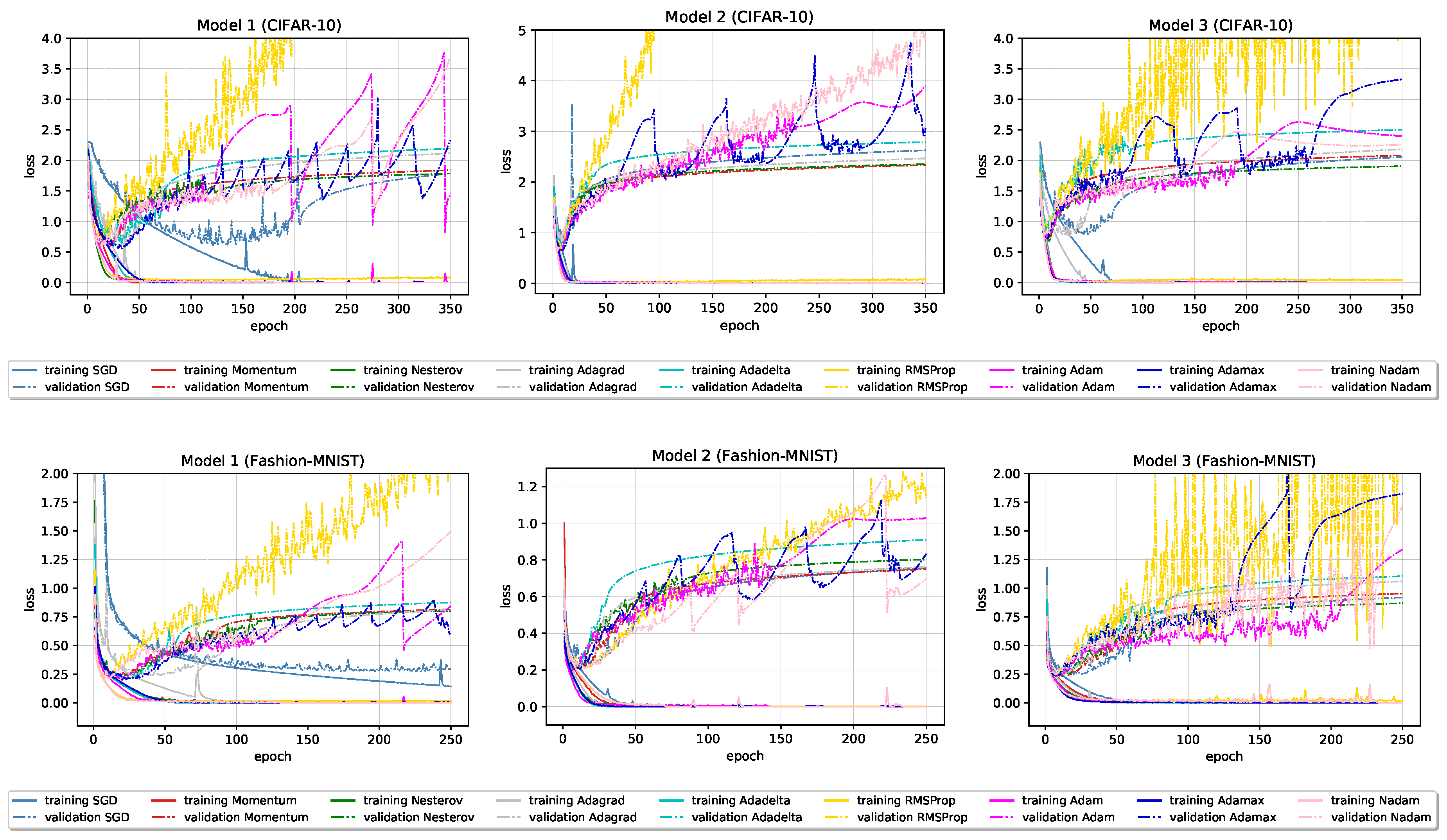
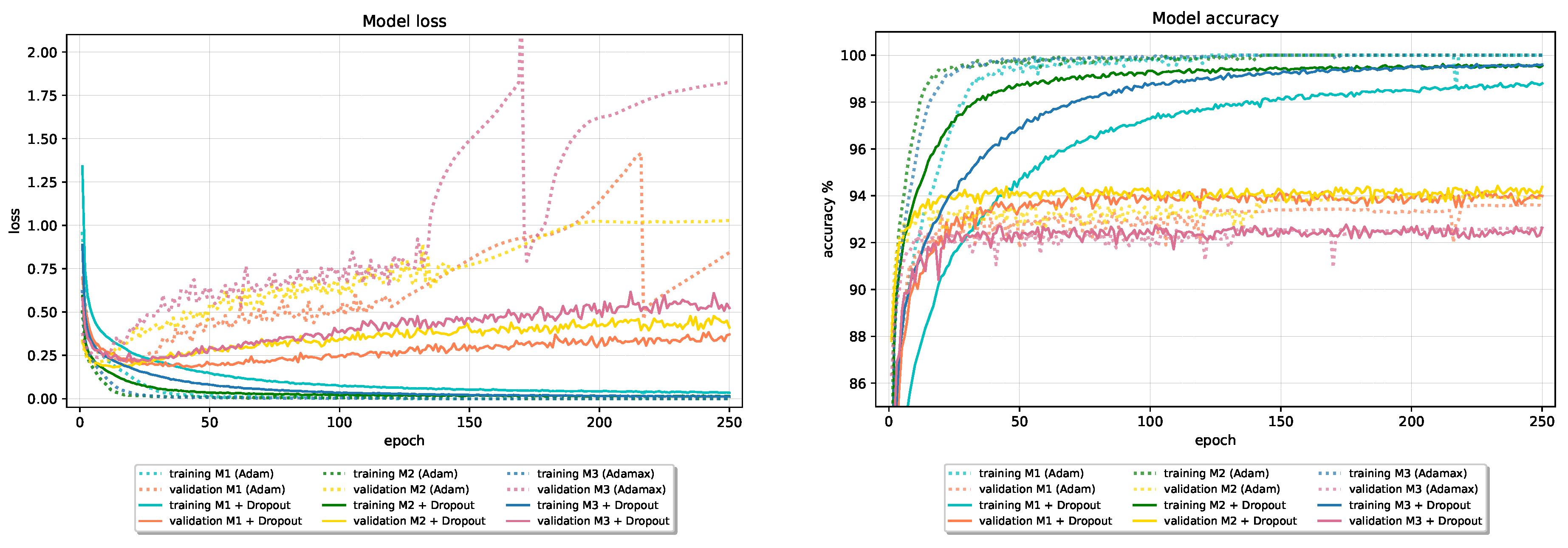
The following observations about the influence of used optimization algorithm on the behavior and final generalization performance of the CNN model are based on their empirical evaluations on three different model architectures, each trained on two datasets with the nine distinct optimizers reviewed in Section 2. Hyperparameters of optimizers used for training each model are given in Appendix B. Figure 3 and Figure 4 show loss and accuracy learning curves of given models, and the final results on the test and training set are reported in

Table 2. Performance of baseline models trained with different optimizers on CIFAR-10 dataset.

	Model 1				Model 2				Model 3
Optimizer	Loss		Accuracy (%)		Loss		Accuracy (%)		Loss		Accuracy (%)
	Train	Test	Train	Test	Train	Test	Train	Test	Train	Test	Train	Test
SGD	$2.25\times {10}^{-4}$	$1.803$	$100.00$	$80.61$	$7.15\times {10}^{-6}$	2.688	$100.00$	$76.49$	$7.73\times {10}^{-5}$	$2.119$	$100.00$	$76.25$
Momentum	$2.65\times {10}^{-6}$	1.926	$100.00$	$83.17$	$1.36\times {10}^{-6}$	2.442	$100.00$	$78.37$	$8.37\times {10}^{-7}$	2.171	$100.00$	$79.23$
NAG	$5.64\times {10}^{-7}$	1.516	100.00	83.68	$9.79\times {10}^{-7}$	2.434	$100.00$	79.11	$5.87\times {10}^{-7}$	2.007	$100.00$	80.40
Adagrad	$1.38\times {10}^{-5}$	2.105	100.00	82.20	$3.65\times {10}^{-6}$	2.586	$100.00$	$77.49$	$4.13\times {10}^{-5}$	2.269	$100.00$	$77.38$
Adadelta	$4.94\times {10}^{-7}$	2.218	100.00	83.65	$1.92\times {10}^{-7}$	$2.884$	$100.00$	$79.09$	$1.32\times {10}^{-7}$	$2.567$	$100.00$	$78.46$
RMSProp	$9.02\times {10}^{-2}$	9.545	99.34	82.04	$7.59\times {10}^{-2}$	$35.001$	99.79	$78.99$	$4.74\times {10}^{-2}$	$4.064$	99.39	$76.37$
Adam	$5.86\times {10}^{-5}$	1.528	100.00	82.93	$2.00\times {10}^{-10}$	$3.893$	$100.00$	79.84	$2.86\times {10}^{-11}$	$2.517$	$100.00$	$79.07$
AdaMax	$6.95\times {10}^{-9}$	2.341	100.00	82.83	$4.33\times {10}^{-4}$	3.119	$99.99$	$78.44$	$0.00\times {10}^0$	3.405	$100.00$	$80.61$
Nadam	$9.63\times {10}^{-10}$	3.807	100.00	82.24	$5.00\times {10}^{-3}$	4.925	$100.00$	$78.65$	$0.00\times {10}^0$	$2.400$	$100.00$	$80.09$

and

Table 3. Performance of baseline models trained with different optimizers on Fashion-MNIST dataset.

	Model 1				Model 2				Model 3
Optimizer	Loss		Accuracy (%)		Loss		Accuracy (%)		Loss		Accuracy (%)
	Train	Test	Train	Test	Train	Test	Train	Test	Train	Test	Train	Test
SGD	$1.25\times {10}^{-1}$	0.353	$95.43$	$89.64$	$1.34\times {10}^{-5}$	0.833	$100.00$	$92.43$	$1.13\times {10}^{-5}$	$0.954$	$100.00$	$91.88$
Momentum	$1.36\times {10}^{-6}$	0.845	$100.00$	$92.54$	$3.58\times {10}^{-6}$	0.779	$100.00$	$92.81$	$1.35\times {10}^{-6}$	1.022	$100.00$	$92.13$
NAG	$1.09\times {10}^{-6}$	0.842	100.00	92.66	$5.82\times {10}^{-7}$	0.863	$100.00$	93.34	$5.38\times {10}^{-7}$	0.937	$100.00$	92.27
Adagrad	$4.34\times {10}^{-5}$	0.940	100.00	91.46	$5.57\times {10}^{-6}$	0.852	$100.00$	$92.62$	$1.93\times {10}^{-6}$	1.139	$100.00$	$91.53$
Adadelta	$7.82\times {10}^{-7}$	0.947	100.00	93.11	$5.13\times {10}^{-7}$	$0.961$	$100.00$	$93.20$	$1.41\times {10}^{-7}$	$1.142$	$100.00$	$92.19$
RMSProp	$1.72\times {10}^{-2}$	2.965	99.81	92.32	$4.06\times {10}^{-4}$	$1.219$	99.99	$92.60$	$1.64\times {10}^{-2}$	$2.211$	$99.73$	$91.05$
Adam	$5.84\times {10}^{-8}$	0.920	100.00	93.27	$1.27\times {10}^{-10}$	$1.029$	$100.00$	93.53	$1.01\times {10}^{-9}$	$1.328$	$100.00$	$92.56$
AdaMax	$9.93\times {10}^{-5}$	0.664	100.00	92.90	$6.41\times {10}^{-8}$	0.964	$100.00$	$93.32$	$0.00\times {10}^0$	$1.790$	$100.00$	92.58
Nadam	$7.95\times {10}^{-11}$	1.662	100.00	93.00	$3.61\times {10}^{-6}$	0.755	$100.00$	$93.01$	$2.46\times {10}^{-7}$	$1.770$	$100.00$	$91.62$

.

The following observations are made:

• The best test set results, in terms of accuracy, are obtained using the classical Nesterov optimization algorithm and adaptive optimization algorithm Adam and its variant AdaMax.
• Compared to Nesterov optimization algorithm, Adam and AdaMax show less stable performance (with many “jumps”) on validation data. The most stable, not necessarily the best, performance on validation data, especially loss, among adaptive optimizers show Adagrad and Adadelta optimization algorithms.
• RMSProp optimization algorithm, in all six cases, has considerably larger validation loss than other optimizers that consistently keeps growing. Interestingly, despite great discrepancy between RMSProp and others optimizers losses, its validation, and finally test set accuracy remains reasonable well and comparable with others.
• In terms of test set accuracy, the ranking of classical optimizers stays consistent across all six models; Nesterov ranked as best, followed by Momentum, and SGD at last. Ranking of adaptive optimizers places Adagrad optimizer on last place, closely followed by RMSProp optimizer.
• Most of the optimizers in 350 epochs succeeded in reaching the ≈0 loss and ≈100% accuracy on the training data in all six models. Exceptions can be found in SGD and RMSProp optimizers, with the overall worst performance obtained by SGD with 95.43% training accuracy.
• In the early stages, especially on Model 2 and Model 3 (Fashion-MNIST), all optimizers beside SGD on Model 1 show signs of overfitting. A large gap between accuracies on the training and new data is noticeable during the whole training process.

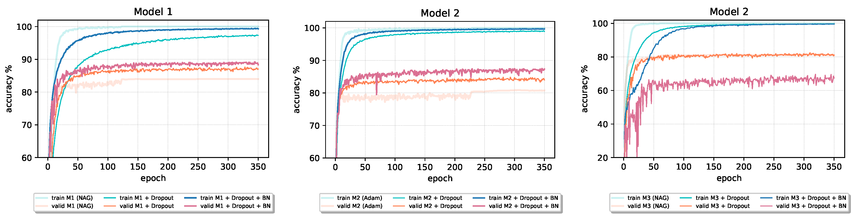
In the rest of the article, we examine how incorporating different regularization methods and Batch Normalization technique affect generalization performance of a given model. For further investigation, we used one optimizer and model architecture per each dataset. Namely, on CIFAR-10 data, we used Nesterov optimizer with first model architecture, Adam with the second and again Nesterov with the third one and refer to them as baseline model architectures. Analogously, for further research on Fashion-MNIST data, as basline model architectures we used Model 1 and Model 2 with Adam optimizer and Model 3 architecture with AdaMax optimization algorithm.

• Batch Normalization

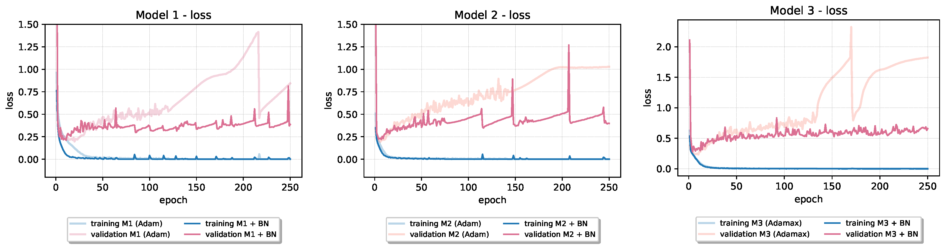
Incorporating Batch Normalization into baseline model architectures, as can be seen in

Table 4. Comparison of results obtained with and without Batch Normalization.

(a) CIFAR-10
Model		Loss		Accuracy (%)
		Train	Test	Train	Test
1.	NAG	$5.64\times {10}^{-7}$	1.516	100.00	83.68
	+ BatchNorm	$2.34\times {10}^{-5}$	0.728	100.00	86.45
2.	Adam	$2.00\times {10}^{-10}$	$3.893$	$100.00$	79.84
	+ BatchNorm	$8.96\times {10}^{-5}$	2.203	100.00	82.89
3.	NAG	$5.87\times {10}^{-7}$	2.007	$100.00$	80.40
	+ BatchNorm	$2.25\times {10}^{-6}$	1.633	$100.00$	81.21
(b) Fashion-MNIST
Model		Loss		Accuracy (%)
		Train	Test	Train	Test
1.	Adam	$5.84\times {10}^{-4}$	0.920	100.00	93.27
	+ BatchNorm	$1.70\times {10}^{-3}$	0.405	99.96	93.25
2.	Adam	$1.27\times {10}^{-10}$	$1.029$	$100.00$	93.53
	+ BatchNorm	$6.10\times {10}^{-5}$	0.455	100.00	93.61
3.	AdaMax	$0.00\times {10}^0$	$1.790$	$100.00$	92.58
	+ BatchNorm	$1.20\times {10}^{-3}$	0.724	$99.96$	91.85

, showed beneficial effects on their final generalization performance. In all cases, the test set loss is significantly reduced, while accuracy on test data increased in four out of six baseline models. In Figure 5 and Figure 6, we can see how validation loss learning curve in all cases significantly drops below the original one. In models that use Adam optimization algorithm for training (Model 2 on CIFAR-10 and Models 1 and 2 on Fashion-MNIST), we can see jumps in the values of both training and validation loss (“spikes” on the learning curves). Even with those kinds of instabilities, the validation loss is still improved over the baseline’s original one. On the training loss curve for the first model architecture, we can se how Batch Normalization can accelerate convergence. From given learning curves, we also notice that overfitting reduced in all cases. Because of that, Batch Normalization is sometimes referred to as an optimization technique with regularizing effect.

4.2.2. Evaluation of Different Regularization Techniques

In this section, we add different types of regularization into the chosen baseline model architectures to examine their effect on the model’s generalization performance.

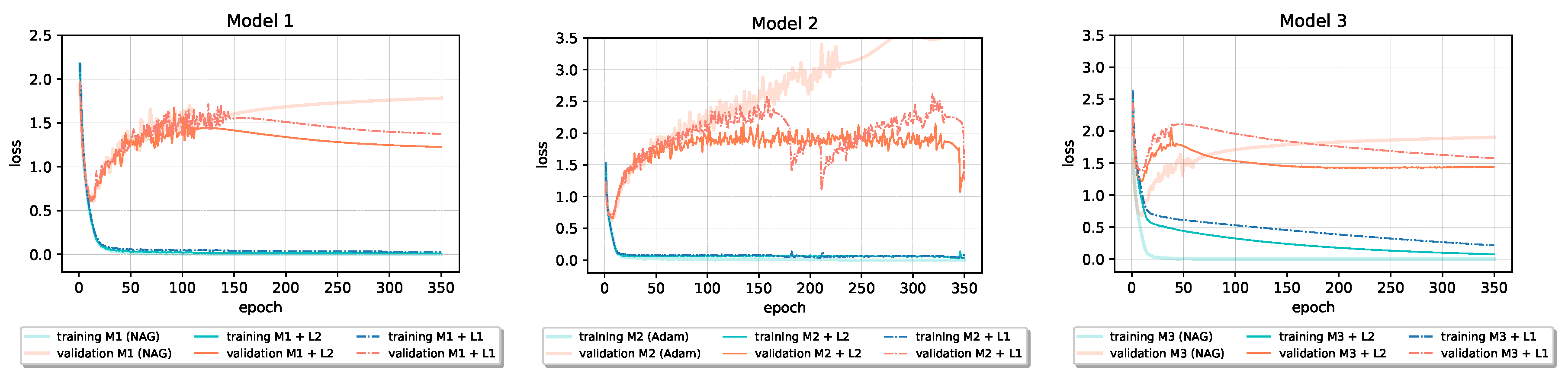
Weight Decay

Adding $L_2$ and $L_1$ regularization into the baseline models did not, in general, result in the improvement of generalization performance. As we can see in

Table 5. Performance of models that use weight decay regularization.

(a) CIFAR-10
Model		Loss		Accuracy (%)
		Train	Test	Train	Test
1.	NAG	$5.64\times {10}^{-7}$	1.516	100.00	83.68
	$L_2$, $\lambda =5\times {10}^{-6}$	$1.26\times {10}^{-2}$	13.615	100.00	83.33
	$L_1$, $\lambda ={10}^{-6}$	$2.99\times {10}^{-2}$	1.477	100.00	83.83
2.	Adam	$2.00\times {10}^{-10}$	$3.893$	$100.00$	79.84
	$L_2$, $\lambda ={10}^{-5}$	$2.90\times {10}^{-2}$	1.483	100.00	79.94
	$L_1$, $\lambda ={10}^{-6}$	$9.27\times {10}^{-2}$	1.339	100.00	76.40
3.	NAG	$5.87\times {10}^{-7}$	2.007	$100.00$	80.40
	$L_2$, $\lambda ={10}^{-5}$	$7.76\times {10}^{-2}$	1.569	100.00	80.70
	$L_1$, $\lambda ={10}^{-6}$	$2.15\times {10}^{-1}$	1.650	100.00	79.99
(b) Fashion-MNIST
Model		Loss		Accuracy (%)
		Train	Test	Train	Test
1.	Adam	$5.84\times {10}^{-4}$	0.920	100.00	93.27
	$L_2$, $\lambda =5\times {10}^{-6}$	$2.90\times {10}^{-2}$	0.593	100.00	92.96
	$L_1$, $\lambda =5\times {10}^{-6}$	$5.37\times {10}^{-2}$	0.515	99.66	92.05
2.	Adam	$1.27\times {10}^{-10}$	$1.029$	$100.00$	93.53
	$L_2$, $\lambda =5\times {10}^{-5}$	$3.64\times {10}^{-2}$	0.462	99.69	92.11
	$L_1$, $\lambda ={10}^{-6}$	$1.51\times {10}^{-2}$	0.670	100.00	93.20
3.	AdaMax	$0.00\times {10}^0$	$1.790$	$100.00$	92.58
	$L_2$, $\lambda ={10}^{-6}$	$2.50\times {10}^{-2}$	0.843	100.00	92.39
	$L_1$, $\lambda ={10}^{-6}$	$1.61\times {10}^{-2}$	0.581	99.98	91.99

, on the Fashion-MNIST dataset, neither $L_2$ nor $L_1$ regularization leads to an increase in the test set accuracy. However, applying $L_1$ regularization on the CIFAR-10 leads to increased accuracy and decreased loss on the test data in baseline Model 1, while adding $L_2$ regularization has beneficial effect on the performance of baseline Models 2 and 3. As parameter $\lambda$, for both $L_2$ and $L_1$ regularization, the best performing value on the validation set from a predefined set of $\lambda$ values $\{{10}^{-2},{10}^{-3},{10}^{-4},{10}^{-5},{10}^{-6}\}$ was chosen. If two neighbor values were close in performance on validation data, we additionally investigated the performance of their midpoint on validation data as potential value for the $\lambda$ parameter. Figure 7 and Figure 8 show that both $L_2$ and $L_1$ regularization reduce all six models’ validation loss during the training. In the third model in Figure 7, penalizing models’ weights notably slows down the convergence; the model needs more than 300 epochs to reach the loss that the baseline model reached before epoch 50. However, after epoch 200, the penalized model’s validation loss falls below the baseline’s validation loss despite the slower learning process.

From the results in Figure 9 and

Table 6. Summary statistics of absolute values of weights.

	${\mathit{L}}_2$	${\mathit{L}}_1$	NAG
min	$4.8\times {10}^{-8}$	0	$5.57\times {10}^{-8}$
$1st$ quartile	$7.49\times {10}^{-5}$	$7.02\times {10}^{-10}$	$1.34\times {10}^{-4}$
median	$1.47\times {10}^{-4}$	$2.12\times {10}^{-9}$	$2.73\times {10}^{-4}$
$3rd$ quartile	$2.22\times {10}^{-4}$	$3.54\times {10}^{-9}$	$2.74\times {10}^{-4}$
max	3.5251	6.6516	2.3028
mean	0.0216	0.0076	0.0349
std	0.0275	0.0426	0.0321

, we can gain insight into the effect that added weight penalties have on final model weights. Obtained results justify the name weight decay; in both cases, resulting weights of regularized models are closer to 0 than the baseline (Model 1 with used NAG optimizer) weights. Most weights of the model that uses $L_1$ regularization are ≈0; the obtained model has sparse weights.

Interestingly, the $L_1$ model has the most dispersed weights and the widest range of absolute values of weights. This can be seen as feature selection; in each layer, weights that correspond to irrelevant features are set to ≈0 while the more important features are emphasized by increasing their (absolute) value and, in that way, also increasing their influence on the final output. $L_2$ regularization has a similar effect. The main difference is that in the case of $L_2$ regularization less important weights are “pulled” towards 0 but not really set to 0.

Noise Injection

Adding (Gaussian) noise to input images did not, in general, result in improved generalization performance. We experimented with different amounts of added noise, Gaussian noise with standard deviation $\sigma \in \{0.01,0.05,0.1,0.2\}$. The final model was trained with parameter $\sigma$ that had the best performance on validation data. Examples of noise injected images from CIFAR-10 and Fashion-MNIST data are shown in Figure 10. Results are given in

Table 7. Results of adding Gaussian noise into the baseline models.

(a) CIFAR-10
Model		Loss		Accuracy (%)
		Train	Test	Train	Test
1.	NAG	$5.64\times {10}^{-7}$	1.516	100.00	83.68
	Noise, $\sigma =0.05$	$1.01\times {10}^{-2}$	19.875	99.74	80.70
2.	Adam	$2.00\times {10}^{-10}$	3.893	$100.00$	79.84
	Noise, $\sigma =0.01$	$9.30\times {10}^{-3}$	4.305	99.77	78.57
3.	NAG	$5.87\times {10}^{-7}$	2.007	$100.00$	80.40
	Noise, $\sigma =0.01$	$6.17\times {10}^{-3}$	2.111	$100.00$	80.42
(b) Fashion-MNIST
Model		Loss		Accuracy (%)
		Train	Test	Train	Test
1.	Adam	$5.84\times {10}^{-4}$	0.920	100.00	93.27
	Noise, $\sigma =0.01$	$1.92\times {10}^{-1}$	0.649	100.00	92.92
2.	Adam	$1.27\times {10}^{-10}$	1.029	$100.00$	93.53
	Noise, $\sigma =0.01$	$5.40\times {10}^{-3}$	11.151	$99.86$	92.63
3.	AdaMax	$0.00\times {10}^0$	$1.790$	$100.00$	92.58
	Noise, $\sigma =0.05$	$2.90\times {10}^{-3}$	0.910	$99.95$	90.95

. Only in one case, we observe slight improvement in the test set accuracy, while accuracy on the training set remains close to $100\%$. Adding noise makes real classes harder to separate. Models have the capacity to learn available training data (training accuracy is in the worst case reduced to 99.74%), but the learned separation criterion also captures the injected noise.

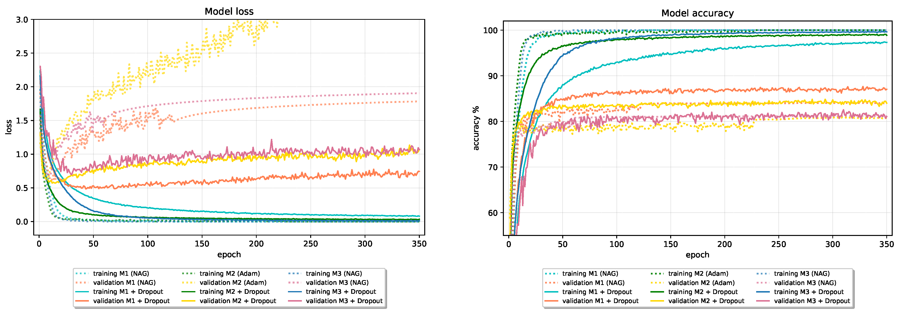
Dropout

By adding Dropout into the baseline models, generalization performance improves. Dropping units during training introduces a significant amount of regularization into the model and greatly reduces signs of overfitting. As we can see in Figure 11 and Figure 12, validation loss of all models on both CIFAR-10 and Fashion-MNIST reduces at the expense of slower convergence and slightly worse final performance on the training data. In

Table 8. Performance of models that employ Dropout regularization.

(a) CIFAR-10
Model	Loss		Accuracy (%)
	Train	Test	Train	Test
1. NAG	$5.64\times {10}^{-7}$	1.516	100.00	83.68
Dropout	$8.10\times {10}^{-2}$	0.754	97.31	86.54
Dropout + inputs	$1.11\times {10}^{-1}$	0.700	96.51	85.38
Dropout + BatchNorm	$2.00\times {10}^{-2}$	0.748	99.34	88.25
2. Adam	$2.00\times {10}^{-10}$	$3.893$	$100.00$	79.84
Dropout	$3.49\times {10}^{-2}$	0.728	98.89	83.64
Dropout + inputs	$3.90\times {10}^{-2}$	1.128	98.72	80.77
Dropout + BatchNorm	$9.9\times {10}^{-3}$	0.904	99.66	86.33
3. NAG	$5.87\times {10}^{-7}$	2.007	$100.00$	80.40
Dropout	$1.08\times {10}^{-2}$	1.099	99.63	80.50
Dropout + inputs	$1.22\times {10}^{-2}$	1.056	99.63	81.26
Dropout + BatchNorm	$1.22\times {10}^{-2}$	522.8	99.59	67.22
(b) Fashion-MNIST
Model	Loss		Accuracy (%)
	Train	Test	Train	Test
1. Adam	$5.84\times {10}^{-4}$	0.920	100.00	93.27
Dropout	$3.41\times {10}^{-2}$	0.471	98.79	93.59
Dropout+ inputs	$6.76\times {10}^{-2}$	0.346	97.55	93.32
Dropout + BatchNorm	$1.13\times {10}^{-2}$	0.412	99.66	93.84
2. Adam	$1.27\times {10}^{-10}$	1.029	$100.00$	93.53
Dropout	$1.46\times {10}^{-2}$	0.485	99.55	93.88
Dropout + inputs	$2.11\times {10}^{-2}$	0.465	99.27	93.21
Dropout + BatchNorm	$6.60\times {10}^{-3}$	0.434	99.77	94.25
3. AdaMax	$0.00\times {10}^0$	$1.790$	$100.00$	l92.58
Dropout	$1.18\times {10}^{-2}$	0.576	99.60	92.01
Dropout + inputs	$1.18\times {10}^{-2}$	0.638	99.62	92.04
Dropout + BatchNorm	$8.10\times {10}^{-3}$	0.612	99.75	92.12

, we give results obtained with models using Dropout compared to baseline models’ results. All models use Dropout with parameter $p=0.5$ on the hidden layers and $p=0.1$ on the input layer, which were chosen using the validation data.

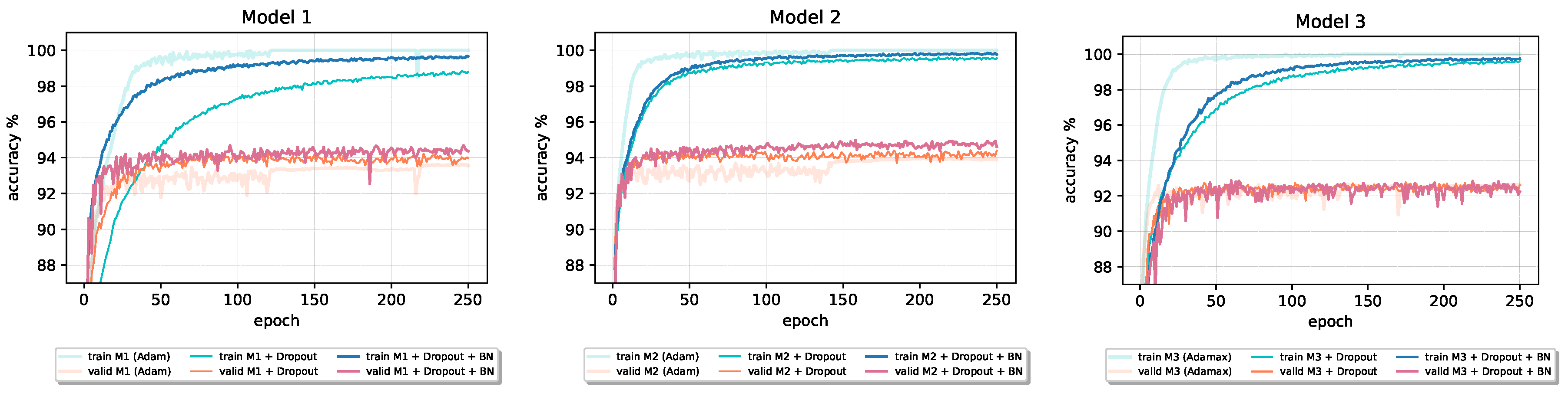
Although the original paper [20] states that Batch Normalization fulfills some of the goals of Dropout and therefore removes the need for using the Dropout regularization method, from the results reported in Table 8 and the accuracy learning curves in Figure 13 and Figure 14 (Model 1 and Model 2), we can see that the combination of these two techniques can benefit final performance of a given model. In all four cases, both validation and training accuracy increase compared to the only Dropout model. Batch Normalization inclusion into Model 1 and Model 2 also speeds up the learning process. However, in the case of Model 3 with the largest number of parameters, Dropout–Batch Norm combination indeed harms the model’s final classification performance. In Figure 13, the validation accuracy learning curve of Model 3 significantly drops when we introduce Batch Normalization together with the Dropout.

Although the accuracy results in Table 8 of the most models that use Dropout with the dropping of input units are lower than those that drop only units in the hidden layers, dropping of input units can play an important role in the generalization performance of the network. To demonstrate how the dropping of input units can positively affect the final performance, we construct a new test set consisting of images from the original CIFAR-10 and Fashion-MNIST test sets with some missing pixel values. The new test sets are obtained by setting 10% of random pixel values from each image to 0. A few examples are shown in Figure 15.

On the new CIFAR-10 test set, (NAG) Model 1, which used the Dropout method without dropping input units, achieves 13.47% accuracy, while final evaluation of the model that dropped inputs with probability p = 0.1 during the training results with 81.28% accuracy on new data. On the new Fashion-MNIST test set, (Adam) Model 1 that incorporates Dropout only on hidden units achieves 83.21% accuracy, while the accuracy of one that drops inputs is equal to 93.17%.

Data Augmentation

During the training, we augmented CIFAR-10 images using horizontal flipping, width and height shifting, random zooming and shearing. For Fashion-MNIST augmentation, we used horizontal flipping and random zooming. Figure 16 shows examples of corresponding augmented images for a given image from CIFAR-10 and Fashion-MNIST data.

Table 9. Results obtained using Data Augmentation technique.

(a) CIFAR-10
Model	Loss		Accuracy (%)
	Train	Test	Train	Test
1. NAG	$5.64\times {10}^{-7}$	1.516	100.00	83.68
DataAugm	$4.51\times {10}^{-2}$	0.887	98.48	87.73
DataAugm + BatchNorm	$1.57\times {10}^{-2}$	0.748	99.49	89.54
DataAugm + Dropout	$1.61\times {10}^{-1}$	0.640	94.74	89.27
DataAugm + BatchNorm + Dropout	$6.38\times {10}^{-2}$	0.655	97.85	89.15
2. Adam	$2.00\times {10}^{-10}$	$3.893$	$100.00$	79.84
DataAugm	$8.06\times {10}^{-2}$	0.728	97.33	86.99
DataAugm + BatchNorm	$3.80\times {10}^{-2}$	0.673	98.74	88.54
DataAugm + Dropout	$1.54\times {10}^{-1}$	0.649	94.74	86.10
DataAugm + BatchNorm + Dropout	$9.06\times {10}^{-2}$	0.519	96.78	88.67
3. NAG	$5.87\times {10}^{-7}$	2.007	$100.00$	80.40
DataAugm	$1.88\times {10}^{-2}$	0.830	99.30	86.98
DataAugm + BatchNorm	$1.66\times {10}^{-2}$	0.966	99.41	85.00
DataAugm + Dropout	$5.72\times {10}^{-2}$	0.713	98.04	86.19
DataAugm + BatchNorm + Dropout	$2.48\times {10}^{-1}$	12723	94.88	80.58
(b) Fashion-MNIST
Model	Loss		Accuracy (%)
	Train	Test	Train	Test
1. Adam	$5.84\times {10}^{-4}$	0.920	100.00	93.27
DataAugm	$1.18\times {10}^{-2}$	0.634	99.59	92.58
DataAugm + BatchNorm	$5.30\times {10}^{-3}$	0.431	99.81	93.49
DataAugm + Dropout	$8.93\times {10}^{-3}$	0.267	96.82	93.92
DataAugm + BatchNorm + Dropout	$3.79\times {10}^{-2}$	0.283	98.62	94.53
2. Adam	$1.27\times {10}^{-10}$	1.029	$100.00$	93.53
DataAugm	$7.70\times {10}^{-3}$	0.726	99.77	93.88
DataAugm + BatchNorm	$4.00\times {10}^{-3}$	0.443	99.87	94.17
DataAugm + Dropout	$4.12\times {10}^{-2}$	0.312	98.59	94.32
DataAugm + BatchNorm + Dropout	$2.09\times {10}^{-2}$	0.291	99.26	94.60
3. AdaMax	$0.00\times {10}^0$	$1.790$	$100.00$	92.58
DataAugm	$4.40\times {10}^{-3}$	0.758	99.88	92.78
DataAugm + BatchNorm	$2.80\times {10}^{-3}$	0.508	99.91	92.77
DataAugm + Dropout	$5.71\times {10}^{-2}$	0.372	97.96	92.54
DataAugm + BatchNorm + Dropout	$3.55\times {10}^{-2}$	0.409	98.72	92.20

gives the results of models that incorporate Data Augmentation compared with the initial baseline results obtained without regularization. Training with augmented data in all cases leads to enhanced model performance. The positive effect of Data Augmentation on generalization performance is more noticeable on CIFAR-10 data than on Fashion-MNIST data due to its large variations in the position of objects on images and background clutter. Including Data Augmentation in the training pipeline alone leads to an increased test set accuracy on CIFAR-10 data for 5.86 in the worst case. Combining Data Augmentation with Batch Normalization and Dropout in Model 1 and Model 2 further improves generalization performance. On CIFAR-10 data, Dropout with parameter $p=0.25$ is used combined with Data Augmentation, while $p=0.5$ is used in the case of the Fashion-MNIST data. Figure 17 and Figure 18 show the effect of Data Augmentation on the learning curves of models trained on CIFAR-10 and Fashion-MNIST data; augmentation reduces validation loss and increases validation accuracy at the expense of slower convergence and worse results on the training data.

Early Stopping

Figure 3 shows how validation loss of all models trained with different optimizers (all optimizers except slower-converging SGD optimizer) even before epoch 50 reaches its minimum value and afterward only increases. Moreover, Figure 4 shows that there is also no specific improvement in validation accuracy after epoch 100 for the most optimizers. Therefore, we could stop the model’s training earlier and obtain model with roughly the same generalization ability. To reduce the training time and prevent possible overfitting to the training data, we used the Early Stopping method with patience 30 to stop the training if there was no improvement in the validation accuracy for 30 consecutive epochs. The model with weights that correspond to the best-observed validation accuracy is returned as a result of the training algorithm.

The other metric that could be monitored during the training and used for decision making about the appropriate time of ending the training algorithm is validation loss. It would be also reasonable to stop the training (with some patience) when the increase in the validation loss is observed. Because we are primarily interested in the accuracy of the final model, we decided to monitor validation accuracy (during the training, we minimize loss instead of maximizing accuracy because the loss function has some “nice” properties such as differentiability).

The final accuracy obtained by models that use Early Stopping and those that do not are compared in

Table 10. Comparison of the accuracy results obtained with and without Early Stopping.

. Although model accuracy on new data is enhanced in some cases, it is often the case that performance of models that use Early Stopping on test data declines. However, training time significantly reduces. For achieving better final accuracy, we can use the larger values for the patience parameter. In some sense, the Early Stopping method can be seen as the trade-off between the time of training and the final performance of the model. For example, the accuracy of Model 1 trained on CIFAR-10 data with Dropout regularization decreases from 87.73% to 84.51% when Early Stopping is used, but training time reduces more than two times. If the training time is not a problem, the model can be trained for longer with saving the parameters that resulted in the best values of a monitored quantity. In Table 10, we can also see how the Data Augmentation technique yields the best accuracy results compared to other previously mentioned “good performing” models that incorporate only one regularizer.

Ensemble Learning

• Bagging
  Let ${\mathcal{D}}_1,\cdots ,{\mathcal{D}}_5$ be datasets of size 40,000 obtained by random sampling with replacement from the CIFAR-10 or Fashion-MNIST training dataset. A Baseline Learner (BL) that has the same architecture as the chosen model is trained on dataset ${\mathcal{D}}_i$, $i=1,\cdots ,5$. $\mathit{Ensi}$ denotes the ensemble $\{BL1,BL2,\dots ,BLi\}$ of the first i baseline learners.
  Each model from the bagged ensemble has accuracy lower than the accuracy of the baselines noted in the last rows of

  Table 11. Bagging results of baseline models on CIFAR 10 dataset.

  and

  Table 12. Bagging results of baseline models on MNIST-Fashion dataset.

  caused by the less diverse training dataset, which contain multiple identical images, but together they outperform the baseline. Each ensemble has better generalization performance than any of its members. Accuracy of ensemble increases together with its size. Generalization performance of models that obtained the highest accuracy on test data further increases when we apply the bagging technique, as shown in

  Table 13. Bagging results applied on the best models on: (a) CIFAR-10 dataset (NAG model that incorporates Data Augmentation and Batch Normalization); and (b) Fashion-MNIST dataset (Adam model that uses Data Augmentation, Batch Normalization and Dropout regularization methods.).

  . The downside of the Bagging method is the additional time necessary to train all of the base learners to obtain desired enhancement in generalization performance.
• The ensemble of members trained with different settings
  Below, we examine how ensembling models with different architectures and settings (in terms of used regularization and optimization techniques) affect the ensemble’s generalization performance compared to the bagging ensembling approach.
  Final accuracies of such ensembles on CIFAR-10 and Fashion-MNIST data are given in

  Table 14. Ensemble of models with different architectures and incorporated regularization techniques.

  . Baseline learners used for CIFAR-10 image classification in Table 14a are Model 3 (NAG + Data Augmentation), Model 1 (NAG + Data Augmentation + Batch Normalization), Model 2 (Adam + Data Augmentation + Batch Normalization), Model 1 (NAG + Dropout), and Model 2 (Adam + Dropout + Batch Normalization). For Fashion-MNIST baseline learners given in Table 14ab are Model 1 (Adam + Dropout + Batch Normalization), Model 2 (Adam + Data Augmentation + Batch Normalization), Model 3 (Data Augmentation), Model 2 (Adam + Data Augmentation + Batch Normalization + Dropout) and Model 1 (Adam + Data Augmentation + Batch Normalization + Dropout). The ensemble formed of “different” members outperforms bagged ensemble created using the one model with the best generalization performance among the “different” ones.

5. Conclusions

In this paper, we summarize different optimization algorithms and regularization methods commonly used for training deep model architectures. The empirical analysis was conducted to quantify and interpret the effect of employed optimization algorithm and regularization techniques on the model’s generalization performance on image classification problem. Provided theoretical background accompanied by experimental results of the learning process can be beneficial to anyone who seeks more in-depth insight into the fields of optimization and regularization of deep learning. When possible, visualizations are used together with experimental evaluations to corroborate claims and intuitions about the effect of mentioned methods on the learning process and model’s final performance on new data.

Empirical evaluations suggest that the optimization algorithm alone can positively affect model’s generalization performance. Nesterov and Adam optimization algorithms were the best-performing algorithms on new data in most of our settings. However, none of the optimization algorithms should be discarded a priori; the evaluation is advisable to select the most appropriate one for the given architecture and dataset problem at hand. Generalization performance can notably be enhanced with proper regularization. Regularization techniques from which implemented CNN architectures gained the most significant improvement in generalization performance were Data Augmentation and Dropout. An appropriate combination of regularization techniques can lead to an even greater boost in the model’s final generalization performance. Batch Normalization, an optimization method with a regularizing effect, seems to work well in combination with the Data Augmentation technique. In our experimental settings, the largest generalization gain was obtained using the combination of Batch Normalization and Data Augmentation together with the Dropout regularization method. However, one should combine Batch Normalization and Dropout with caution since their combination can result with an underperformance. If we want to improve generalization performance further, training multiple models to form an ensemble can be beneficial (given the availability of computational resources). To speed up the training and still obtain a model with reasonable generalization performance, the Early Stopping method can be used.

It is important to mention some limitations of conducted evaluations. In this work, regularization is used to complement the optimizer’s performance to explore the extent to which the generalization performance can be improved, thus focusing on the evaluation of regularization techniques on the best optimizer per each of three CNN architectures and two benchmark datasets. It would be interesting to expand the experimental evaluations to examine the extent to which the regularizers would yield favorable results with other lower-performing optimizers. Most of the mentioned techniques are applicable to a wide range of problems. Therefore, it would be interesting to extend their experimental evaluations on different neural network architectures and problems from different domains. Further research within this scope could include a more detailed examination of the techniques associated with the optimization, such as the learning rate schedules, different weight initialization schemes, and their effect on the generalization performance.

References

- Liu, Y.; Wang, Y.; Wang, S.; Liang, T.; Zhao, Q.; Tang, Z.; Ling, H. Cbnet: A novel composite backbone network architecture for object detection. arXiv 2019, arXiv:1909.03625. [Google Scholar] [CrossRef]
- Chen, L.C.; Zhu, Y.; Papandreou, G.; Schroff, F.; Adam, H. Encoder-decoder with atrous separable convolution for semantic image segmentation. In Proceedings of the European Conference on Computer Vision (ECCV), Munich, Germany, 8–14 September 2018; pp. 801–818. [Google Scholar]
- Saon, G.; Kurata, G.; Sercu, T.; Audhkhasi, K.; Thomas, S.; Dimitriadis, D.; Cui, X.; Ramabhadran, B.; Picheny, M.; Lim, L.L.; et al. English conversational telephone speech recognition by humans and machines. arXiv 2017, arXiv:1703.02136. [Google Scholar]
- Edunov, S.; Ott, M.; Auli, M.; Grangier, D. Understanding back-translation at scale. arXiv 2018, arXiv:1808.09381. [Google Scholar]
- Dai, Z.; Yang, Z.; Yang, Y.; Carbonell, J.; Le, Q.V.; Salakhutdinov, R. Transformer-xl: Attentive language models beyond a fixed-length context. arXiv 2019, arXiv:1901.02860. [Google Scholar]
- Zhang, C.; Bengio, S.; Hardt, M.; Recht, B.; Vinyals, O. Understanding deep learning requires rethinking generalization. arXiv 2017, arXiv:1611.03530. [Google Scholar]
- Dogo, E.; Afolabi, O.; Nwulu, N.; Twala, B.; Aigbavboa, C. A comparative analysis of gradient descent-based optimization algorithms on convolutional neural networks. In Proceedings of the 2018 International Conference on Computational Techniques, Electronics and Mechanical Systems (CTEMS), Belgaum, India, 21–22 December 2018; pp. 92–99. [Google Scholar]
- Choi, D.; Shallue, C.J.; Nado, Z.; Lee, J.; Maddison, C.J.; Dahl, G.E. On empirical comparisons of optimizers for deep learning. arXiv 2019, arXiv:1910.05446. [Google Scholar]
- Bera, S.; Shrivastava, V.K. Analysis of various optimizers on deep convolutional neural network model in the application of hyperspectral remote sensing image classification. Int. J. Remote Sens. 2020, 41, 2664–2683. [Google Scholar] [CrossRef]
- Kandel, I.; Castelli, M.; Popovič, A. Comparative Study of First Order Optimizers for Image Classification Using Convolutional Neural Networks on Histopathology Images. J. Imaging 2020, 6, 92. [Google Scholar] [CrossRef]
- Soydaner, D. A Comparison of Optimization Algorithms for Deep Learning. Int. J. Pattern Recognit. Artif. Intell. 2020, 2052013. [Google Scholar] [CrossRef]
- Smirnov, E.A.; Timoshenko, D.M.; Andrianov, S.N. Comparison of regularization methods for imagenet classification with deep convolutional neural networks. Aasri Procedia 2014, 6, 89–94. [Google Scholar] [CrossRef]
- Nusrat, I.; Jang, S.B. A comparison of regularization techniques in deep neural networks. Symmetry 2018, 10, 648. [Google Scholar] [CrossRef]
- Garbin, C.; Zhu, X.; Marques, O. Dropout vs. batch normalization: An empirical study of their impact to deep learning. Multimed. Tools Appl. 2020, 79, 1–39. [Google Scholar] [CrossRef]
- Chen, G.; Chen, P.; Shi, Y.; Hsieh, C.Y.; Liao, B.; Zhang, S. Rethinking the Usage of Batch Normalization and Dropout in the Training of Deep Neural Networks. arXiv 2019, arXiv:1905.05928. [Google Scholar]
- Simonyan, K.; Zisserman, A. Very deep convolutional networks for large-scale image recognition. arXiv 2014, arXiv:1409.1556. [Google Scholar]
- Kukačka, J.; Golkov, V.; Cremers, D. Regularization for deep learning: A taxonomy. arXiv 2017, arXiv:1710.10686. [Google Scholar]
- Krizhevsky, A.; Nair, V.; Hinton, G. CIFAR-10 (Canadian Institute for Advanced Research). Available online: http://www.cs.toronto.edu/kriz/cifar.html (accessed on 29 August 2020).
- Xiao, H.; Rasul, K.; Vollgraf, R. Fashion-mnist: A novel image dataset for benchmarking machine learning algorithms. arXiv 2017, arXiv:1708.07747. [Google Scholar]
- Ioffe, S.; Szegedy, C. Batch normalization: Accelerating deep network training by reducing internal covariate shift. arXiv 2015, arXiv:1502.03167. [Google Scholar]
- Robbins, H.; Monro, S. A stochastic approximation method. Ann. Math. Stat. 1951, 22, 400–407. [Google Scholar] [CrossRef]
- Polyak, B.T. Some methods of speeding up the convergence of iteration methods. USSR Comput. Math. Math. Phys. 1964, 4, 1–17. [Google Scholar] [CrossRef]
- Nesterov, Y.E. A method for solving the convex programming problem with convergence rate O (1/k2). Dokl. Akad. Nauk Sssr 1983, 269, 543–547. [Google Scholar]
- Duchi, J.; Hazan, E.; Singer, Y. Adaptive subgradient methods for online learning and stochastic optimization. J. Mach. Learn. Res. 2011, 12, 2121–2159. [Google Scholar]
- Zeiler, M.D. Adadelta: An adaptive learning rate method. arXiv 2012, arXiv:1212.5701. [Google Scholar]
- Tieleman, T.; Hinton, G. Lecture 6.5-rmsprop: Divide the gradient by a running average of its recent magnitude. COURSERA Neural Netw. Mach. Learn. 2012, 4, 26–31. [Google Scholar]
- Graves, A. Generating sequences with recurrent neural networks. arXiv 2013, arXiv:1308.0850. [Google Scholar]
- Kingma, D.P.; Ba, J. Adam: A method for stochastic optimization. arXiv 2014, arXiv:1412.6980. [Google Scholar]
- Dozat, T. Incorporating Nesterov Momentum into Adam. 2016. Available online: http://cs229.stanford.edu/proj2015/054_report.pdf (accessed on 29 August 2020).
- Sutskever, I.; Martens, J.; Dahl, G.; Hinton, G. On the importance of initialization and momentum in deep learning. In Proceedings of the International Conference on Machine Learning, Atlanta, GA, USA, 16–21 June 2013; pp. 1139–1147. [Google Scholar]
- Goodfellow, I.; Bengio, Y.; Courville, A. Deep Learning; MIT Press: Cambridge, MA, USA, 2016; Available online: http://www.deeplearningbook.org (accessed on 29 August 2020).
- Srivastava, N.; Hinton, G.; Krizhevsky, A.; Sutskever, I.; Salakhutdinov, R. Dropout: A simple way to prevent neural networks from overfitting. J. Mach. Learn. Res. 2014, 15, 1929–1958. [Google Scholar]
- Breiman, L. Bagging predictors. Mach. Learn. 1996, 24, 123–140. [Google Scholar] [CrossRef]
- Prechelt, L. Early stopping-but when? In Neural Networks: Tricks of the Trade; Springer: Berlin/Heidelberg, Germany, 1998; pp. 55–69. [Google Scholar]
- Springenberg, J.T.; Dosovitskiy, A.; Brox, T.; Riedmiller, M. Striving for simplicity: The all convolutional net. arXiv 2014, arXiv:1412.6806. [Google Scholar]
- Krizhevsky, A.; Sutskever, I.; Hinton, G.E. Imagenet classification with deep convolutional neural networks. In Advances in Neural Information Processing Systems; NIPS’12 Conference Organizer: Lake Tahoe, Nevada, 2012; pp. 1097–1105. [Google Scholar]
Figure 1.
Dropout during the training (left) and testing phase (right).
Figure 2.
Bagging scheme.
Figure 3.
Loss learning curves for all optimizers on baseline models.
Figure 4.
Accuracy learning curves for all optimizers on baseline models.
Figure 5.
The effect of Batch Normalization on the loss of baseline models trained on CIFAR-10 dataset.
Figure 6.
The effect of Batch Normalization on the loss of baseline models trained on Fashion-MNIST dataset.
Figure 7.
Loss learning curves of models that incorporate and weight decay in baseline models trained on CIFAR-10 dataset.
Figure 8.
Loss learning curves of models that incorporate and weight decay in baseline models trained on Fashion-MNIST dataset.
Figure 9.
Comparison of baseline’s weights with weights obtained by models that use weight decay regularization methods with regularization parameter .
Figure 10.
Images with different amounts of added noise
Figure 11.
The effect of Dropout on baseline models trained on CIFAR-10 dataset.
Figure 12.
The effect of Dropout on baseline models trained on Fashion-MNIST dataset.
Figure 13.
The effect of the Batch Normalization on the accuracy of models trained on the CIFAR-10 dataset that incorporate Dropout regularization.
Figure 14.
The effect of the Batch Normalization on the accuracy of models trained on the Fashion-MNIST dataset that incorporate Dropout regularization.
Figure 15.
Examples from new CIFAR-10 (top) and Fashion-MNIST (bottom) test sets with missing pixel values.
Figure 16.
Examples of augmented images.
Figure 17.
The effect of Data Augmentation on baseline models trained on CIFAR-10 dataset.
Figure 18.
The effect of Data Augmentation on baseline models trained on Fashion-MNIST dataset.