Article

Transfer Learning-Based Fault Diagnosis under Data Deficiency

1
Department of Aerospace and Mechanical Engineering, Korea Aerospace University, Goyang 10540, Korea
2
Department of Mechanical and Aerospace Engineering, University of Florida, Gainesville, FL 32611, USA
3
School of Aerospace and Mechanical Engineering, Korea Aerospace University, Goyang 10540, Korea
*
Author to whom correspondence should be addressed.
Appl. Sci. 2020, 10(21), 7768; https://doi.org/10.3390/app10217768
Submission received: 4 September 2020 / Revised: 20 October 2020 / Accepted: 30 October 2020 / Published: 3 November 2020
(This article belongs to the Special Issue Advances in Machine Fault Diagnosis)

Abstract

:
In the fault diagnosis study, data deficiency, meaning that the fault data for the training are scarce, is often encountered, and it may deteriorate the performance of the fault diagnosis greatly. To solve this issue, the transfer learning (TL) approach is employed to exploit the neural network (NN) trained in another (source) domain where enough fault data are available in order to improve the NN performance of the real (target) domain. While there have been similar attempts of TL in the literature to solve the imbalance issue, they were about the sample imbalance between the source and target domain, whereas the present study considers the imbalance between the normal and fault data. To illustrate this, normal and fault datasets are acquired from the linear motion guide, in which the data at high and low speeds represent the real operation (target) and maintenance inspection (source), respectively. The effect of data deficiency is studied by reducing the number of fault data in the target domain, and comparing the performance of TL, which exploits the knowledge of the source domain and the ordinary machine learning (ML) approach without it. By examining the accuracy of the fault diagnosis as a function of imbalance ratio, it is found that the lower bound and interquartile range (IQR) of the accuracy are improved greatly by employing the TL approach. Therefore, it can be concluded that TL is truly more effective than the ordinary ML when there is a large imbalance between the fault and normal data, such as smaller than 0.1.

1. Introduction

In recent years, fault diagnosis of mechanical components has been studied very actively and many important advances have been made primarily based on the machine learning techniques such as k-nearest neighbor (KNN) [1], support vector machine (SVM) [2], convolutional neural network (CNN) [3], and others. However, these research techniques have dealt with situations where training and test data lie in the same domain with enough amounts of fault data. While this unusual situation enables the diagnosis performance more superior, it does not reflect the circumstances of the real field where the fault diagnosis should be carried out under a lack of fault data due to cost and safety issues.
In the study of Prognostics and Health Management (PHM), the lack of fault or failure data, which is referred to as the “data deficiency”, has been considered as the main obstacle that deteriorates the performance of PHM. To tackle this issue, there have been several efforts with different perspectives and strategies. For example, Kim et al. [4] proposed data augmentation prognostics (DAPROG) by augmenting the run-to-fail (RTF) data obtained in the past for various operating conditions to the current one using dynamic time warping (DTW). Sobie et al. [5] generated virtual training data exploiting the high-resolution simulations based on the roller bearing dynamics and improved the machine learning classification performance. A data fusion approach was also proposed as a means to compensate the absence of data in certain classes, which are addressed by Diez-Olivan et al. [6], with reviews and challenges for the industrial prognosis; Azamfar et al. [7], for the gearbox fault diagnosis using the convolutional neural network (CNN) and motor current signature analysis, Huang et al. [8] for the mechanical fault diagnosis based on IoT; Luwei et al. [9], for the rotating machine fault classification, to name a few.
Over the years, transfer learning (TL) has emerged as one of the solutions. TL is a method of extracting knowledge obtained in one domain (source domain) to solve problems in another domain (target domain), combining with machine learning techniques. The fundamental idea is that if the source and target domain are similar, using the trained weights of the source domain is more efficient than the training of the target domain from scratch. As a result, the TL algorithm compensates for data deficiency in the target domain, such as the insufficient amount and unlabeled samples. Several studies have been made in this direction. For example, Zhang et al. [10] proposed transfer learning based on the neural networks (NN) for multiclass fault diagnosis of rolling bearings. Parameters of the NN in the source domain are obtained through the training phase and transferred to the target task which has more classes to classify. Classification accuracy and training time were improved compared to those by the traditional NN. Wen et al. [11] proposed a new deep transfer learning method for fault diagnosis of different working conditions. They extracted domain-invariant features by using sparse auto-encoder and the maximum mean discrepancy between domains. Compared to the results of traditional methods, such as the deep belief network (DBN), SVM, and artificial neural network (ANN), the proposed method has made good improvement. They have also conducted a comparative study for different ratios of samples between the source and target dataset. Qian et al. proposed a transfer learning-based fault diagnosis network combined with high-order Kullback–Leibler (HKL) divergence [12]. The proposed network has extracted features through the sparse filtering and HKL divergence for discrimination and generalization ability. They have validated their method by both the bearing and gearbox datasets. Lu et al. [13] proposed domain adaptation combined with a deep convolutional generative adversarial network (DA-DCGAN) for the DC series arc fault diagnosis in a photovoltaic (PV) system. They used normal and fault data of the source domain (PV emulator in the laboratory) and only normal data of the target domain (PV system in the field) for an adversarial training process. By generating fault data of the target domain artificially, high detection accuracy was achieved. Guo et al. [14] proposed a deep convolutional transfer learning network (DCTLN) for intelligent fault diagnosis of machines with unlabeled data. They optimized their network models in the direction of minimizing the maximum mean discrepancy (MMD) between the source and target domain datasets for learning domain-invariant features from raw signals.
The above-mentioned papers have shown several improvements in the fault diagnosis by using TL, but the imbalance issue in the sample size between the normal and fault data was not studied, which may affect the performance of TL greatly. Even though a few papers [11,12] have addressed a similar issue, it was about the sample imbalance between the source and target domain, in which the size of fault data is the same or greater than the normal. Recalling that the fault does not occur often in the real operation conditions because of the periodic maintenance or the costly effort to make by intention, the imbalance issue between the normal and fault data is of great importance for practical use. For this reason, the effect of transfer learning in the fault diagnosis of imbalanced data is investigated in this study.

2. Transfer Learning

Transfer learning is to extract knowledge from one domain task and utilize (or transfer) it to solve another domain task. The domain in which knowledge is extracted is referred to as the source domain, and the domain in which the knowledge is transferred is referred to as the target domain. Depending on the type of knowledge and the way it is transferred, transfer learning is divided by several approaches [15]. In this paper, parameter transfer is employed, in which a neural network is trained by the source domain dataset and the pre-trained model is transferred to the target domain to fine-tune its parameters by the target domain dataset. In the parameter transfer-based approach, the source datasets are usually relatively large in sample size while the target datasets are small. The approach assumes that the parameters of the source and target domains share a common part shown as follows [10]:
θ s   =   θ     +     θ 1
θ t   =   θ     + θ 2
where θ denotes parameters, such as weight and bias, of a neural network, and the subscript s and t denote the source and target domain, respectively. The idea is that by initializing the parameters with those of the source domain, the accuracy and training efficiency can be improved substantially [10].
In this paper, the influence of the imbalance ratio in the target domain, defined as the proportion of sample size between normal and fault, is investigated in the transfer learning framework, and compared with the results by the traiditional neural network. As stated before, the motivation of this study is due to the lack of fault data in the real field. The flowchart is presented in Figure 1. As shown in Figure 1a, in the traditional machine learning-based fault diagnosis, datasets of different states (e.g., normal and fault) are divided into the training and test. Training data are used to train a model for the diagnosis and test data to measure the performance of the model. Note in the figure that the degraded dataset is smaller in sample size than that of the normal dataset, which is usually the case in the field, and may be responsible for the poor classification performance. In the transfer learning (TL)-based diagnosis, there are two groups of datasets from the different domains: the source and target as shown in Figure 1b. The former is used to extract knowledge and the latter to utilize the knowledge for its diagnosis. In this case, the degraded dataset in the source domain is relatively larger in sample size than those in the target domain, which is going to be exploited for the diagnosis of the target domain. In this paper, parameter transfer is used so that a neural network (NN) is trained in the source domain and the pre-trained model is transferred to fine-tune the parameter in the target domain. The concept is that the model parameters on the left in the source domain are knowledge-transferred to serve as the initial values of the model on the right in the target domain, which can improve the accuracy and efficiency of training greatly.

3. Application

3.1. Linear Motion Guide Dataset

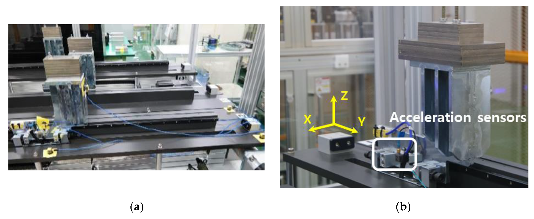
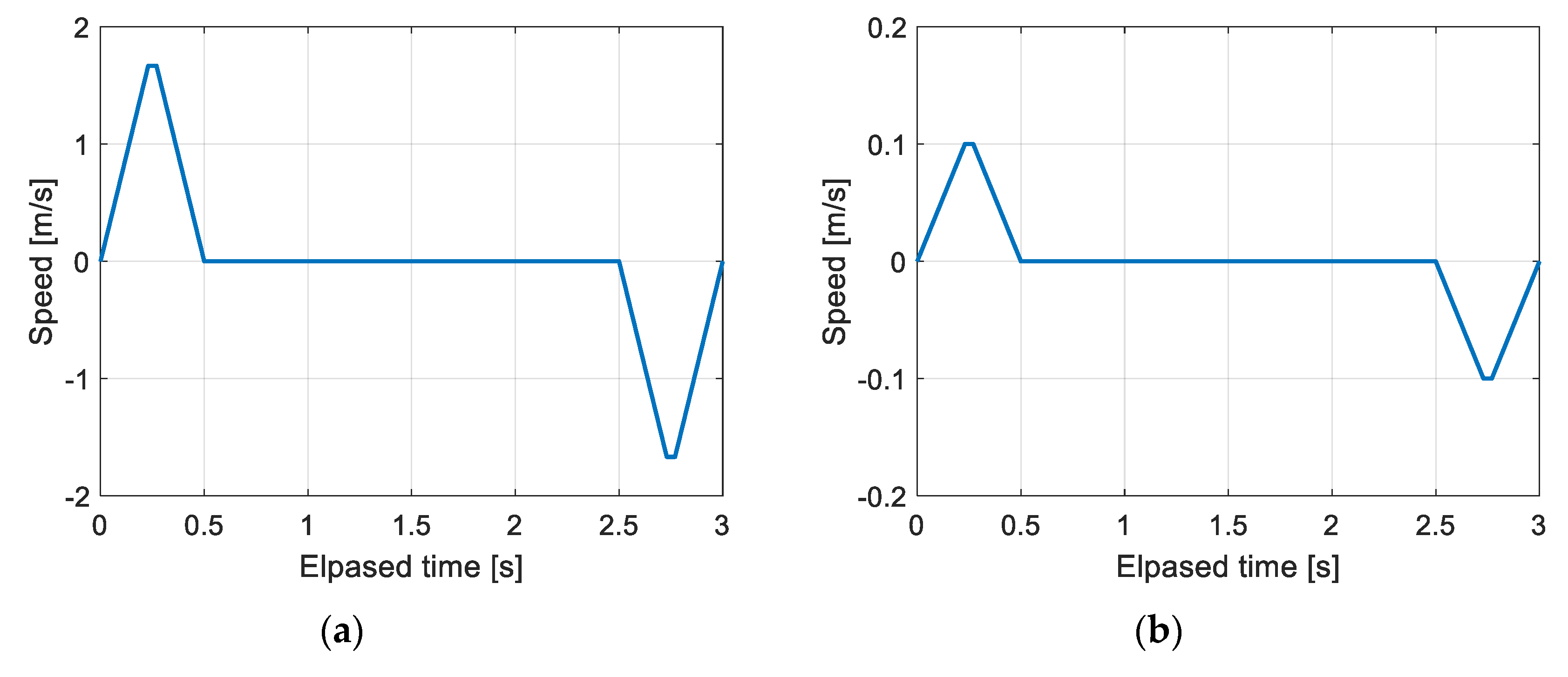
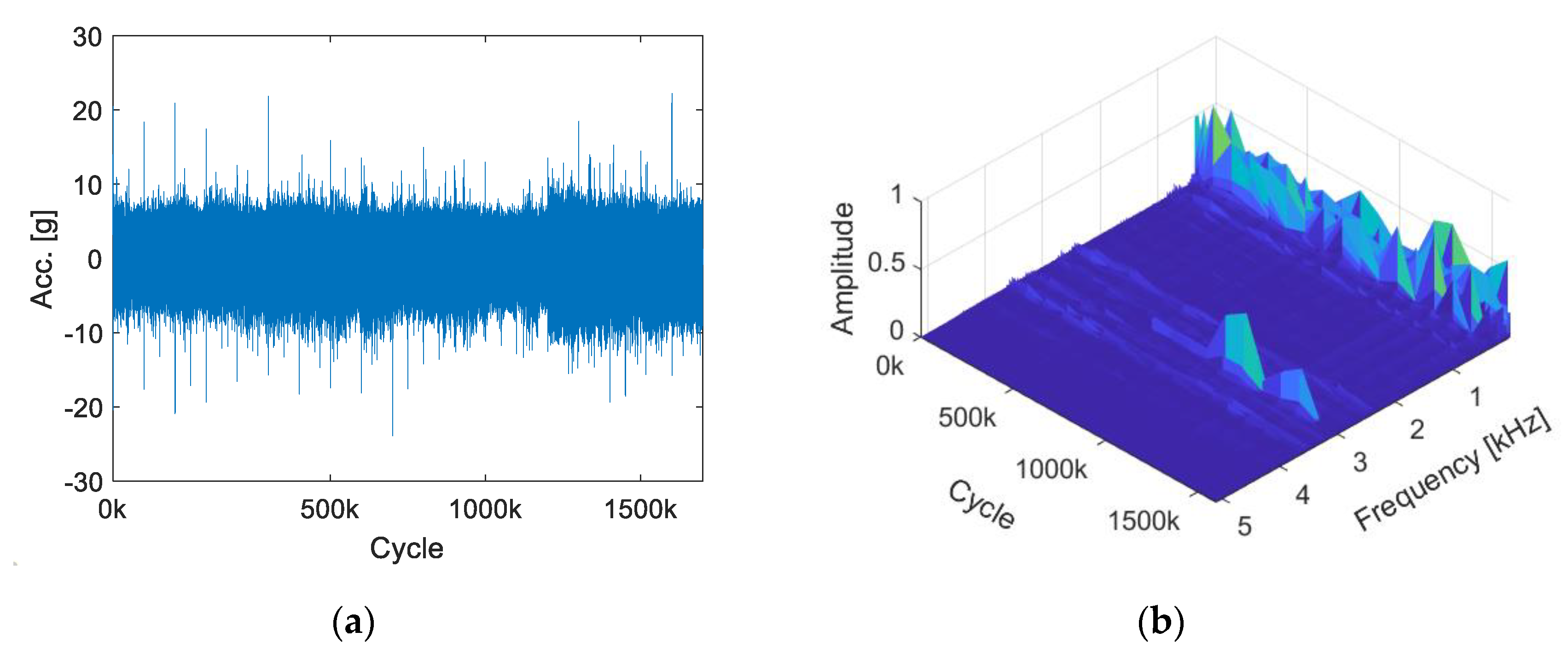
A linear motion (LM) guide is a frequently used mechanical part in the manufacturing field because it moves heavy workpieces while maintaining precision at high speeds. The LM guide in the experiment is a ball guide type with a rectangular LM block whose height and width are 24 mm and 34 mm. Only one LM block is installed in a single rail. The seal type of the LM block is an end seal for dust prevention. The workpiece is fixed to the surface of the LM block, which travels along a linear rail with dozens of balls circulating inside of the block as shown in Figure 2. Since the balls move along the track in the LM block, flaking may occur due to the rolling contact fatigue loads. Four LM guides are prepared, and test rigs are made, which consist of the motor and belt drive (not shown here), rail, workpiece, and LM guides as shown in Figure 3a. The LM block reciprocates along a 450 mm-long rail with a sequence of acceleration for 0.23 s, a constant speed of 1.667 m/s for 0.04 s, and deceleration for 0.23 s, which is shown in Figure 4a. A three-axis accelerometer with a sampling rate of 10.2 kHz is installed at the LM block as shown in Figure 3b. The vibration signal is measured intermittently at the 0, 20 k, 50 k, and 100 k’th cycles for the early period, and at every 100 k cycle for the subsequent period. At each recording cycle, the signal is recorded twice with different speeds: first at the original 1.667 m/s (high) and next at 0.1 m/s (low). This is to simulate the on-line operation during the production and the off-line inspection operation during the maintenance, respectively. The speed profile for the latter case is shown in Figure 4b. In the recording cycle, the measurement is repeated nine or ten times at random under each speed. The experiment is terminated when one of the LM guides encounters the flaking appearance during the inspection, which has taken about two months. As a result, the total number of datasets is given by 680 and 723 for the high and low speeds, respectively, where a dataset refers to the measured data for a single trip. Figure 5a shows the plot of the vibration signal under the low speed over the whole period acquired for one of the LM guides. Figure 5b is its three-dimensional spectrogram, which is the stack of the frequency spectrum made by fast Fourier transform at each cycle. The figure shows that the amplitudes at around 3 kHz increase from a certain time period, which is about the last 25% of the whole cycle. The same phenomena are found in the other LM guides. The authors believe that this represents the fault progression of LM guides, eventually leading to the flaking failure.
Since the data can be easily acquired during the maintenance, the latter is defined as the source domain, whereas the former being the target domain. Then the imbalance condition is considered where the fault data in the target domain are much less available than those in the source domain due to the infrequent occurrence in the real operation. Among the datasets in the source domain (low speed), those in the first six.
Note that 25% and the last 25% of the whole period are chosen as the normal and fault at our convenience to make the number of datasets in each class the same. The results are 152 datasets in common for the normal and fault conditions. Then, the NN is trained using the all the datasets (152 normal samples and 152 fault samples) in the source domain. In the target domain (high speed), the datasets of the normal and fault conditions are chosen in the same way, and the results are 160 datasets in common. Then, the datasets are divided into the training and test, with the number being 100 and 60, respectively. The training datasets are used to train the NN which is pre-trained and transferred from the source domain. The test datasets are used to examine the accuracy of the trained NN. The numbers in each case are summarized in Table 1.
To simulate the imbalance condition where the fault data in the target domain are much less available than those in the source domain, only a part of the fault datasets are taken as shown in Table 1, which is given by multiplying the imbalance ratio (IR). For example, when the IR is set at 0.1, only 10 percent of the fault datasets are used in the target domain for the training.

3.2. Training Neural Networks of Source Domain

As shown in Figure 1, the transfer learning is preceded by the training of the NN in the source domain using the 152 datasets of the normal and fault as given in Table 1. As is addressed in many works of literature (e.g., see [16,17]), the training process consists of the training and validation, in which the training is to determine the parameters (weights and bias) under a given architecture, whereas the validation is to find out the optimum architecture or hyper-parameters that give the best performance.
Thirteen time-domain statistical features as listed in Table 2 are extracted from the raw signals in the three directions, which gives the thirty-nine features. These are used as the input nodes of the NN. In terms of the architecture, a single hidden layer is considered with the transfer function being the hyperbolic tangent sigmoid. The optimum number of nodes in the hidden layer is then sought by the validation process, more specifically the five-fold cross-validation in practice. To this end, the datasets are divided into the five folds, in which the four are used for the training (determining the weights and bias of the network), while the remaining one is used for the validation. The diagnosis accuracy is then calculated by the ratio of the number of correct classifications to the total number of validation datasets. Since there are five folds, this is repeated five times, from which the average accuracy is obtained. Furthermore, since the NN solutions can vary widely due to the random initial conditions, this is repeated 300 times, and the grand average is obtained accordingly. The process is repeated by increasing the number of nodes in the hidden layer from 2 to 100 by increments of 2 (e.g., 2, 4, 6 …, 100). The result of validation in the source domain is given in Figure 6a, where the optimum number of hidden nodes is chosen at 22 by visual inspection. Once this is done, the NN is trained again to obtain the parameters (weights and bias) under the optimum architecture (namely, 22 hidden nodes) using the training datasets with initial values of the parameters given at random. Repeating this by 300 times, 300 sets of parameters are obtained for the NN in the source domain, which we call the pre-trained NN parameters to be used in the target domain. The reason for the repetition is due to the arbitrary nature of the NN solution.

3.3. Training Neural Networks of Target Domain by Transfer Learning

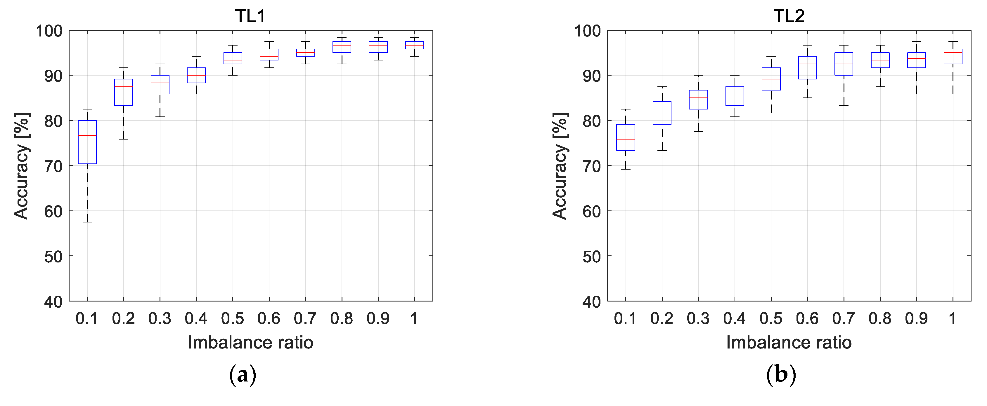
Once the NN is trained in the source domain, it can be exploited by TL in the target domain. There are two ways for this: One is named TL1, which uses the same architecture in the target domain as that of the source domain. The other is TL2, which, in addition to the same architecture, initial values for the training are given by the pre-trained NN parameters of the source domain. Whichever it is, the training is carried out using the architecture of the source domain by 300 times for the training datasets in the target domain as given in Table 1. In the training, the initial values of the parameters are assumed at random in TL1 whereas they are given by the pre-trained NN parameters in TL2. The trained NNs are applied to the test datasets of Table 1, from which the diagnosis accuracies are obtained as defined previously in the source domain. Since the 300 number of accuracy is obtained as a result, the accuracy is represented by the distribution, which occurs due to the randomness of NN solutions. Furthermore, the number of fault datasets vary by IR. So this is repeated for each IR from 0.1 to 1.0 by the increment of 0.1. Note that the smaller the IR, the more the data deficiency becomes greater.
To make a comparison of the TL-based approach, the ordinary machine learning (ML) approach is also performed. In this case, the training and validation are carried out solely by the training datasets in the target domain to determine the optimum architecture. The procedure is the same as that addressed in the source domain. The process is repeated for each IR from 0.1 to 1.0 by the increment of 0.1. Figure 6b gives the result of validation when IR is 0.5, where the optimum number of hidden nodes is found at 16. The results for other IRs are found in Table 3. Once this is done, the NN has trained again by 300 times to obtain the 300 sets of parameters under the architecture using the training datasets with the initial values assumed at random. Finally, the trained NNs are applied to the test datasets of Table 1, from which the diagnosis accuracies are obtained, representing the distribution due to the randomness of NN solutions.
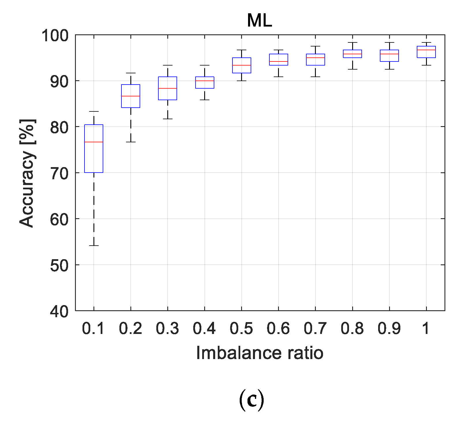
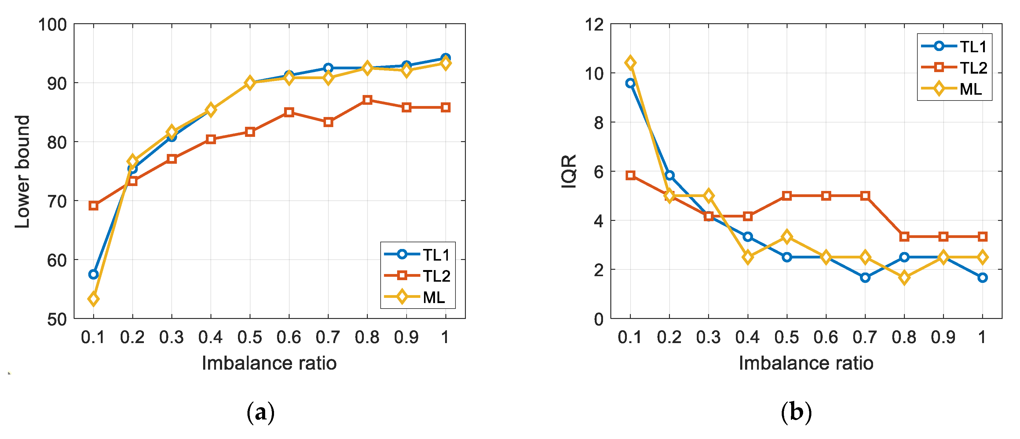
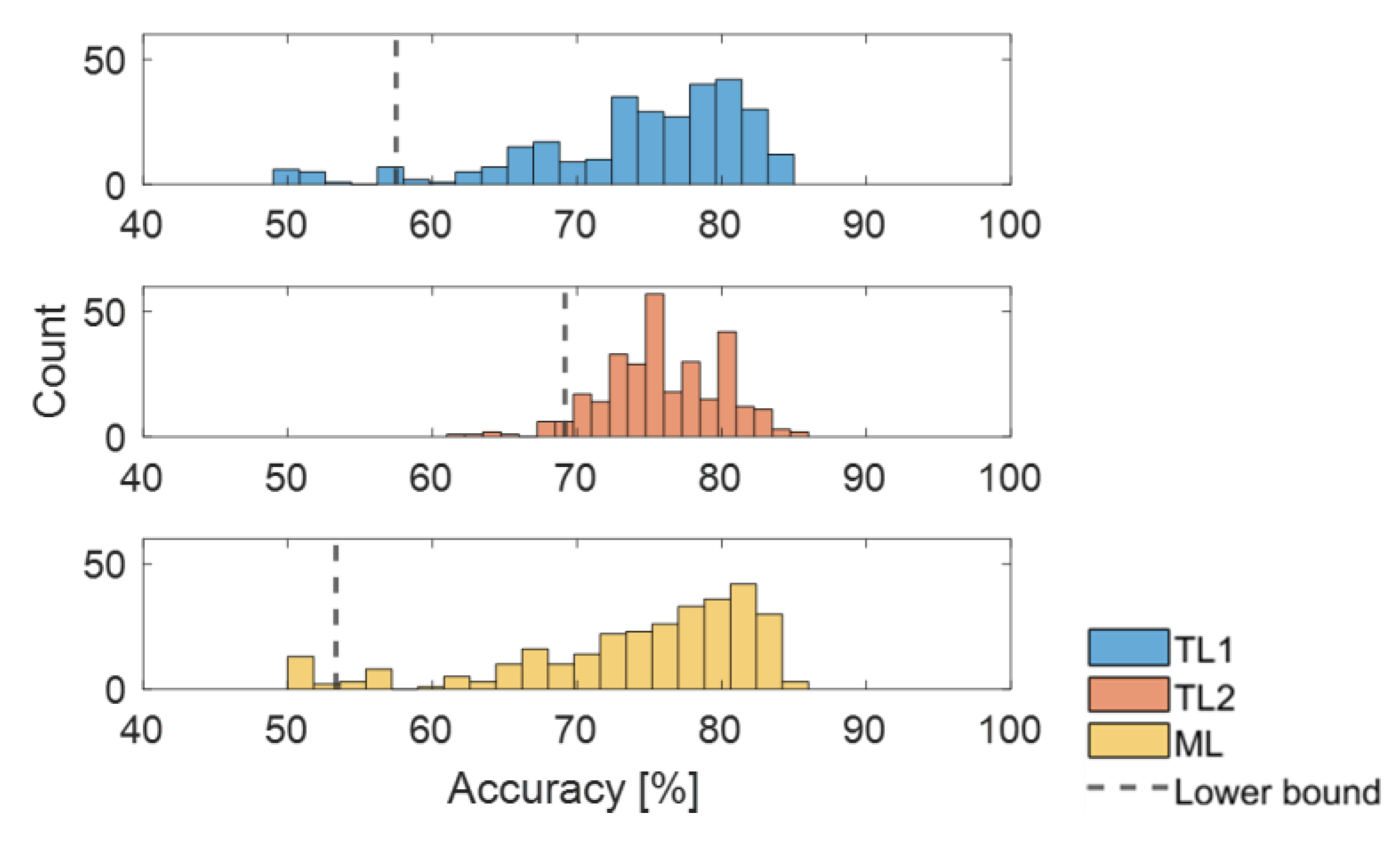
The results of accuracy distribution in TL1, TL2, and ML are given as a function of IR as shown in Figure 7a–c, respectively. In the figures, the bottom, top, and red lines of the box indicate the 25th, 75th percentile, and median of the distribution, respectively. The top and bottom of the extended dotted lines are the 5th and 95th percentiles. In Figure 8a,b, the lower bound (fifth percentile) and the IQR between 25th and 75th percentiles are shown, which indicate the lower confidence limit of accuracy and the degree of statistical dispersion, respectively [18]. When the IR is 0.1, the lower bound of TL2 is 69.2, which is greater than 57.5 (TL1) and 53.3 (ML), and the IQR is 5.83, which is only about 60% of 9.58 (TL1) and 10.41 (ML). The higher the bound and the lower the IQR, the better the performance. This can be identified more clearly in Figure 9, where the histograms of diagnosis accuracy and its lower bound are displayed for TL1, TL2, and ML, respectively. While the histograms of TL1 and ML are similar and show much larger variance, TL2 shows smaller variance with greater lower confidence limit. However, as the IR increases greater than 0.1, the lower bound and IQR of TL2 are not superior to the others. The authors believe that these results are due to the negative transfer [10], which happens when the fault characteristics between the source and target domain are quite different. In that case, adding the fault data in the target domain does not help to improve the TL performance. Overall observations are summarized as follows: (1) TL1 and ML behave similarly, whereas TL2 is different from the others. That is, the initialization of NN parameters is of more importance than the adoption of source domain architecture in making the difference of TL from ordinary ML in the target domain. (2) TL2 is superior to ML and TL1 only when the number of fault data is very small such as when IR is 0.1 or less as is evident in Figure 8, in which the lower bound of accuracy for TL2 is higher and the IQR for TL2 is shorter than the other two. This is why TL is necessary for the case when the data are too few to train by their own. (3) It is of surprise that TL2 is soon found less effective than the other two as the IR gets greater than 0.1. Nevertheless, it should not be overlooked that the proposed approach is truly useful in the case of significant data deficiency, which is the highlight of the study.

4. Conclusions

Collecting the fault data during the real operation is difficult because of safety and cost issues, which results in the imbalance issue in the number of normal versus fault data, and even data deficiency. The performance of fault diagnosis is then greatly deteriorated due to this. On the other hand, a good number of normal and fault data can be acquired in a similar condition such as the lab test or maintenance inspection. In this study, a transfer learning-based fault diagnosis is proposed to solve this problem, which is to pre-train the NN using the large datasets as the source domain, and transfer the knowledge to train the NN using the imbalanced datasets in the real target domain. To illustrate this, normal and fault datasets are acquired from the run-to-fail test of the LM guides, in which the data at high and low speeds are regarded as those for the real operation (target) and maintenance inspection (source), respectively. To study the effect of imbalance, the number of fault data in the target domain is reduced by multiplying the imbalance ratio (IR), and the accuracy of diagnosis is explored as a function of IR. From the study, it is concluded that TL is truly more effective than ordinary ML when there is a large imbalance between the fault and normal such as smaller than 0.1. When the imbalance ratio is 0.1, the variance is improved substantially such that the IQR is about 60% of the others. However, to our surprise, it soon becomes less so, reversing the performance as the IR is increased, which is a too small benefit to employ TL as the solution. This seems to be attributed to the negative transfer arising when the fault characteristics differ too much between the source and target domain. How to figure out and overcome this will be another future research topic, which involves numerous implementations of various experimental datasets.

Author Contributions

Conceptualization, S.H.C. and S.K.; methodology, S.H.C. and S.K.; writing—original draft preparation, S.H.C.; writing—review and editing, J.-H.C.; supervision, J.-H.C. All authors have read and agreed to the published version of the manuscript.

Funding

This work was supported by the National Research Foundation of Korea (NRF) grant funded by the Korea government(MSIT) (No. 2020R1A4A407990411).

Conflicts of Interest

The authors declare no conflict of interest.

References

  1. Bagheri, B.; Ahmadi, H.; Labbafi, R. Application of Data Mining and feature extraction on Intelligent Fault Diagnosis by Artificial Neural Network and K-Nearest Neighbor. In Proceedings of the XIX International Conference on Electrical Machines—ICEM 2010, Rome, Italy, 6–8 September 2010. [Google Scholar] [CrossRef]
  2. Hu, Q.; He, Z.; Zhang, Z.; Zi, Y. Fault diagnosis of rotating machinery based on improved wavelet package transform and SVMs ensemble. Mech. Syst. Signal. Process. 2007, 21, 688–705. [Google Scholar] [CrossRef]
  3. Eren, L.; Ince, T.; Kiranyaz, S. A Generic Intelligent Bearing Fault Diagnosis System Using Compact Adaptive 1D CNN Classifier. J. Signal. Process. Syst. 2019, 91, 179–189. [Google Scholar] [CrossRef]
  4. Kim, S.; Kim, N.H.; Choi, J.-H. Prediction of remaining useful life by data augmentation technique based on dynamic time warping. Mech. Syst. Signal. Process. 2020, 136, 106486. [Google Scholar] [CrossRef]
  5. Sobie, C.; Freitas, C.; Nicolai, M. Simulation-driven machine learning: Bearing fault classification. Mech. Syst. Signal. Process. 2018, 99, 403–419. [Google Scholar] [CrossRef]
  6. Diez-Olivan, A.; Del Ser, J.; Galar, D.; Sierra, B. Data fusion and machine learning for industrial prognosis: Trends and perspectives towards Industry 4.0. Inf. Fusion 2019, 50, 92–111. [Google Scholar] [CrossRef]
  7. Azamfar, M.; Singh, J.; Bravo-Imaz, I.; Lee, J. Multisensor data fusion for gearbox fault diagnosis using 2-D convolutional neural network and motor current signature analysis. Mech. Syst. Signal. Process. 2020, 144, 106861. [Google Scholar] [CrossRef]
  8. Huang, M.; Liu, Z.; Tao, Y. Mechanical fault diagnosis and prediction in IoT based on multi-source sensing data fusion. Simul. Model. Pr. Theory 2020, 102, 101981. [Google Scholar] [CrossRef]
  9. Luwei, K.C.; Yunusa-Kaltungo, A.; Sha’Aban, Y.A. Integrated Fault Detection Framework for Classifying Rotating Machine Faults Using Frequency Domain Data Fusion and Artificial Neural Networks. Machines 2018, 6, 59. [Google Scholar] [CrossRef] [Green Version]
  10. Zhang, R.; Tao, H.; Wu, L.; Guan, Y. Transfer Learning With Neural Networks for Bearing Fault Diagnosis in Changing Working Conditions. IEEE Access 2017, 5, 14347–14357. [Google Scholar] [CrossRef]
  11. Wen, L.; Gao, L.; Li, X. A New Deep Transfer Learning Based on Sparse Auto-Encoder for Fault Diagnosis. IEEE Trans. Syst. Man Cybern. Syst. 2017, 49, 136–144. [Google Scholar] [CrossRef]
  12. Qian, W.; Li, S.; Wang, J. A New Transfer Learning Method and its Application on Rotating Machine Fault Diagnosis under Variant Working Conditions. IEEE Access 2018, 6, 69907–69917. [Google Scholar] [CrossRef]
  13. Lu, S.; Sirojan, T.; Phung, B.T.; Zhang, D.; Ambikairajah, E. DA-DCGAN: An Effective Methodology for DC Series Arc Fault Diagnosis in Photovoltaic Systems. IEEE Access 2019, 7, 45831–45840. [Google Scholar] [CrossRef]
  14. Guo, L.; Lei, Y.; Xing, S.; Yan, T.; Li, N. Deep Convolutional Transfer Learning Network: A New Method for Intelligent Fault Diagnosis of Machines with Unlabeled Data. IEEE Trans. Ind. Electron. 2018, 66, 7316–7325. [Google Scholar] [CrossRef]
  15. Zheng, H.; Wang, R.; Yang, Y.; Yin, J.; Li, Y.; Li, Y.; Xu, M. Cross-Domain Fault Diagnosis Using Knowledge Transfer Strategy: A Review. IEEE Access 2019, 7, 129260–129290. [Google Scholar] [CrossRef]
  16. Bin, G.; Gao, J.; Li, X.; Dhillon, B. Early fault diagnosis of rotating machinery based on wavelet packets—Empirical mode decomposition feature extraction and neural network. Mech. Syst. Signal. Process. 2012, 27, 696–711. [Google Scholar] [CrossRef]
  17. Saravanan, N.; Ramachandran, K. Incipient gear box fault diagnosis using discrete wavelet transform (DWT) for feature extraction and classification using artificial neural network (ANN). Expert Syst. Appl. 2010, 37, 4168–4181. [Google Scholar] [CrossRef]
  18. Buch, K.D. Decision Based Non-Linear Filtering Using Interquartile Range Estimator for Gaussian Signals. In Proceedings of the 2014 Annual IEEE India Conference (INDICON), Pune, India, 11–13 December 2014. [Google Scholar] [CrossRef]
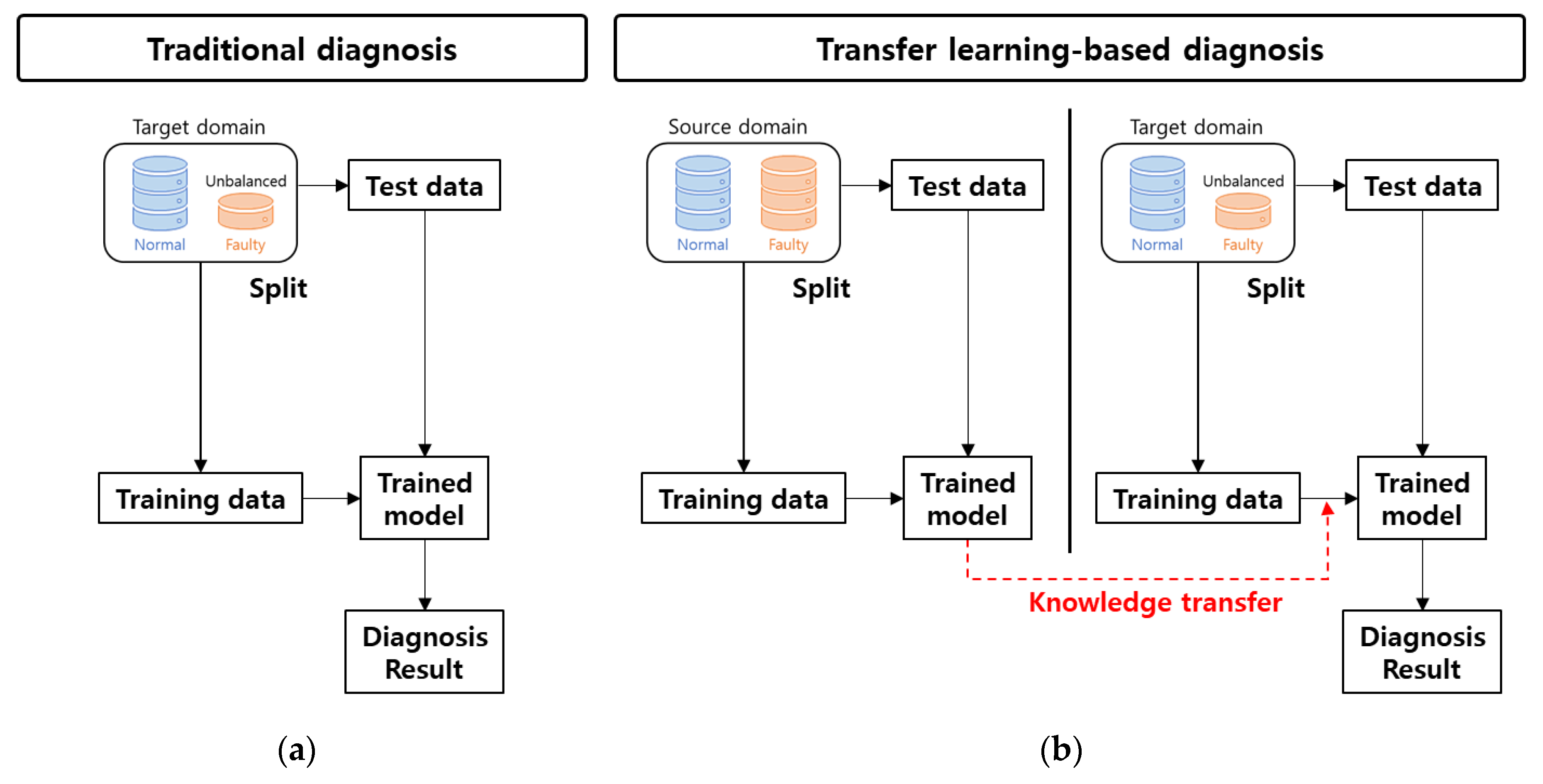
Figure 1. Flowchart of fault diagnosis: (a) traditional machine learning-based approach, and (b) transfer learning-based approach [15].
Applsci 10 07768 g001
Figure 2. Linear motion (LM) guide structure and flaking inside the LM block.
Applsci 10 07768 g002
Figure 3. Experimental setup: (a) linear motion guide test rigs; (b) installed accelerometer.
Applsci 10 07768 g003
Figure 4. Speed profile of LM guide: (a) high speed during production (target domain); (b) low speed during an inspection (source domain).
Applsci 10 07768 g004
Figure 5. Vibration signal of low speed for one of the LM guides: (a) raw signal in time domain; (b) frequency spectrum by Fourier transform.
Applsci 10 07768 g005
Figure 6. Diagnosis accuracy as a function of the number of hidden nodes: (a) the source domain; (b) the target domain with IR of 0.5.
Applsci 10 07768 g006
Figure 7. Diagnosis accuracy of the target domain: (a) transfer learning (TL)1; (b) TL2; (c) machine learning (ML).
Applsci 10 07768 g007aApplsci 10 07768 g007b
Figure 8. Two measures of diagnosis accuracy: (a) lower bound; (b) interquartile range (IQR).
Applsci 10 07768 g008
Figure 9. Histogram of diagnosis accuracy when IR is 0.1.
Applsci 10 07768 g009
Table 1. Details of LM dataset.
PurposeNormal DatasetFault Dataset
Source DomainTraining152152
Target DomainTraining100100*IR 1
Test6060
1 Imbalance ratio (IR) denotes the imbalance ratio.
Table 2. Equations for statistical features.
FeatureFormulaFeatureFormula
Mean 1 N i N x i Crest factor max   ( | x i | ) 1 N i N x i 2
Root amplitude ( 1 N i N | x i | ) 2 Clearance factor max ( | x i | ) ( 1 N i N | x i | ) 2
RMS 1 N i N x i 2 Shape factor 1 N i N x i 2 1 N i N | x i |  
Standard deviation 1 N 1 i N ( x i x ¯ ) 2 Impulse factor max ( | x i | ) 1 N i N | x i |
Peak max ( | x i | ) Peak-to-peak max ( x i ) min ( x i )
Skewness i N ( x i x ¯ ) 3 ( N 1 ) σ 3 Root sum of squares i N x i 2
Kurtosis i N ( x i x ¯ ) 4 ( N 1 ) σ 4
Table 3. The number of nodes in hidden layer determined in the target domain.
IR0.10.20.30.40.50.60.70.80.91.0
The number of nodes in hidden layer10181410161012161212
Publisher’s Note: MDPI stays neutral with regard to jurisdictional claims in published maps and institutional affiliations.