Prediction of Residual Stress of Carburized Steel Based on Machine Learning

Abstract

In recent years, the number of machine learning applications (especially those involving deep learning) applied to predicting and discovering material properties has been increasing. This paper is based on using microstructure and carbon content to train machine learning models to predict the residual stress of carburized steel. First, a semantic segmentation model of the material organization structure (SegModel-MOS) was constructed based on the AlexNet network and initially trained on the PASCAL VOC2012 dataset. Then, the trained model was fine-tuned on an enhanced homemade dataset consisting of optical microstructures. The experimental results show that SegModel-MOS can distinguish acicular martensite, retained austenite, and lath martensite in microstructures. Finally, we used both support vector machine (SVM) and decision tree (DT) algorithms to establish a mapping relationship between the microstructure, carbon content, and residual stress to predict the residual stress of steel from its microstructure and carbon content. The experiments verified that the prediction model constructed in this study exhibits high accuracy and can directly predict residual stress without requiring any long-term measurements. Thus, the developed model provides a new approach to the study of residual stress in steel.

1. Introduction

Carburized steel specimens are subject to complex friction, wear, and cyclic stresses during service. The steel surface is most prone to fatigue failure [1,2,3,4]. Under certain load conditions, the maximum stress of the part is also often generated on the part surface. Therefore, increasing the strength of the surface of a part and increasing its residual compressive stress both play key roles in increasing its fatigue life. Residual compressive stress can suppress the initiation of surface cracks, thereby improving the fatigue life of manufactured parts [5,6]. However, because residual stress field tests are lengthy and damage the component, we instead aimed to predict the residual stress of steel using its microstructure and carbon content based on a data-driven method. This approach can be used to conduct performance analysis for most low-alloy carburized steels. Thus, it provides a new method for research into the performance of carburized steels.

At present, as material databases have increased, many machine learning applications have been developed to predict the mechanical properties of materials. For example, Shen et al. [7], during the heat treatment process, analyzed the alloying elements of steel, which are the parameters that most directly determine structural aspects such as the content and morphology of martensite matrix, retained austenite, and precipitates. An SVM-PM model was built using alloy elements to predict hardness. Ampazis et al. [8] proposed using a support vector machine (SVM) to predict the degradation of mechanical properties of Al2024-T3 aluminum alloy used in aircraft due to surface corrosion. However, both the chemical composition and microstructure of materials determine their mechanical properties. The above studies considered only the influence of chemical composition on mechanical properties; they did not consider the influence of organization on mechanical properties. To establish the relationship among chemical elements, microstructure, and mechanical properties, the microstructure must first be accurately identified. Thus, it is critical to be able to accurately segment photos of steel microstructures [9,10,11,12,13,14,15].

A neural network establishes a mapping from a feature space to a target attribute without considering any complex internal transformation laws; instead, it transforms the process into a set of trainable weights that can theoretically approximate any type of nonlinear transformation. Therefore, an increasing number of researchers have applied neural networks to various image segmentation tasks. In the metallurgical field, Masci et al. [16] used a convolutional neural network (CNN) for segmentation to discover defects in steel and laid the foundation for deep learning to identify microstructures. Later, Bai Long et al. [17] used an SVM to extract the morphological features of cast iron. Dmitry et al. [18] used a random forest (RF) statistical algorithm to identify steel microstructures; their method can process large numbers of images rapidly. Azimi et al. [19] used a fully convolutional neural network (FCNN) to perform pixel-level segmentation of steel microstructures. These studies laid the foundation for the precise segmentation of microstructures.

However, the above studies used convolutional neural networks exclusively to recognize photos acquired by scanning electron microscopy (SEM); they did not address recognizing complex optical photos. Therefore, this study used a fully convolutional neural network combined with transfer learning and residual blocks to semantically segment optical microscopy images [20,21]. During this process, (1) transfer learning was used to solve the problem of insufficient network generalization ability due to fewer training samples, and (2) the residual block prevented overfitting. After the microstructure had been accurately segmented, an SVM classifier was used to predict the residual stress of carburized steel.

According to Northwood et al. [22], the amount of retained austenite and the residual stress increase as the carbon content increases, and they decrease after tempering. Deng et al. [23] found that as the carburizing temperature and carbon potential increase, the amount of carbon in the carburized layer increases, which in turn leads to an increase in residual stress and inhibits the initiation of cracks. Yang et al. [24] studied the calculation model for retained austenite, martensite, and residual stress by using the finite element method under different carburizing processes. The results show that the established model is effective at calculating the residual stress field of the martensitic transformation during the quenching process of the steel specimen. However, the above description stems from only a simple study of the relationship between residual stress and microstructure or residual stress and carbon content; there has been no systematic study of residual stress and microstructure or carbon content. Because residual stress depends primarily on the cooling process, the volume expansion of the martensite transformation caused by the different surface carbon contents expands by different degrees. In addition, after quenching, the surface of the martensite structure is inconsistent with that of the transition layer and the core. Using the C content and the tissue gradient to predict residual stress should improve the accuracy.

In the work detailed in this paper, the carbon content of the surface-to-subsurface areas of the carburized and quenched surfaces of 23CrNi3Mo steel was gradually reduced. The volume expansion caused by martensitic transformation was gradually reduced from the surface to the core, resulting in greater residual compressive stress at the surface than in the core. The material organization structure segmentation model (SegModel-MOS) model used for semantic segmentation of optical micrographs was based on AlexNet and trained with 1200 homemade optical microstructure images. The experimental results demonstrate that SegModel-MOS effectively identifies needle-shaped martensite, residual austenite, and lath martensite from microstructure images. The main contributions of this article are as follows:

• A high-precision semantic segmentation model for optical micrographs, named SegModel-MOS, is established. This model combines migration learning and a residual network to achieve accurate image segmentation after training with small numbers of data samples.
• In this paper, the SVM algorithm is first used to establish a mapping relationship with the residual stress based on the percentage and carbon content of acicular martensite, retained austenite, and lath martensite steel microstructures; then, it predicts the residual stress.

2. Preparation of Optical Microstructure Pictures

2.1. Experimental Process

Five groups of 23CrNi3Mo steel rod-shaped samples with a diameter of 10 mm and a length of 50 mm were selected, and the rod surfaces were polished with 3000 grit sandpaper. The carburizing experiment was performed at a fixed carburizing temperature of 930 °C, but the carburizing times were varied. In

Table 1. Heat treatment process.

	Carburization Processes			Oil Quenching Temperature (°C)	Tempering Temperature (°C)	Tempering Time (h)
	Carburizing Temperature (°C)	Boost Stage Time (h)	Diffusion Stage Time (h)
Process 1	930	2	2	860	200	2
Process 2		2	4
Process 3		3	4
Process 4		4	4
Process 5		6	6

, Processes 1 to 5 are carburizing heat treatment processes. After carburizing was complete, the temperature was reduced to 860 °C for 0.5 h, and then the steel was oil-quenched. The quenching temperature was selected (1) to reduce the sample deformation and (2) to reduce the retained austenite content as much as possible. Thus, 860 °C was used as the quenching temperature based on the phase transformation point, and the sample was maintained at this temperature for 0.5 h to ensure a stable sample temperature. Subsequent tempering was performed at 200 °C for 2 h to obtain a tempered martensite structure, reduce brittleness, and obtain excellent strength and toughness. Generally, a tempering time no longer than 2 h results in minimal alteration of mechanical properties. Therefore, tempering was performed at 200 °C for 2 h. Then, the sample was removed and air-cooled.

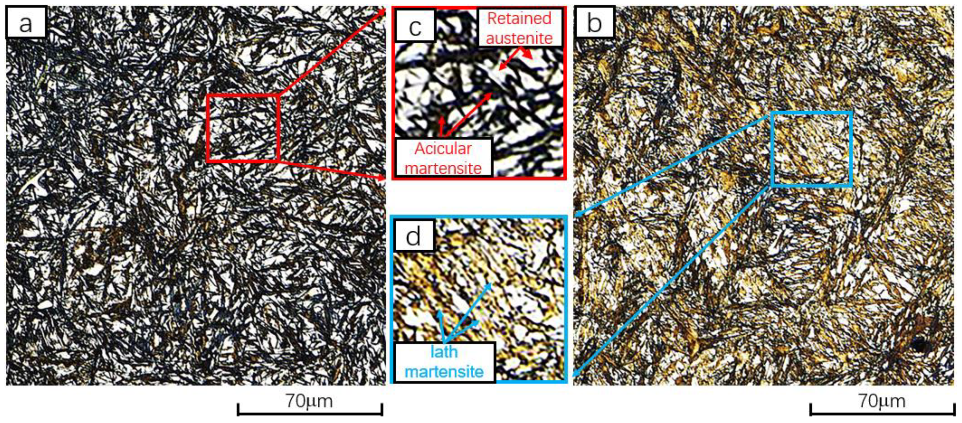
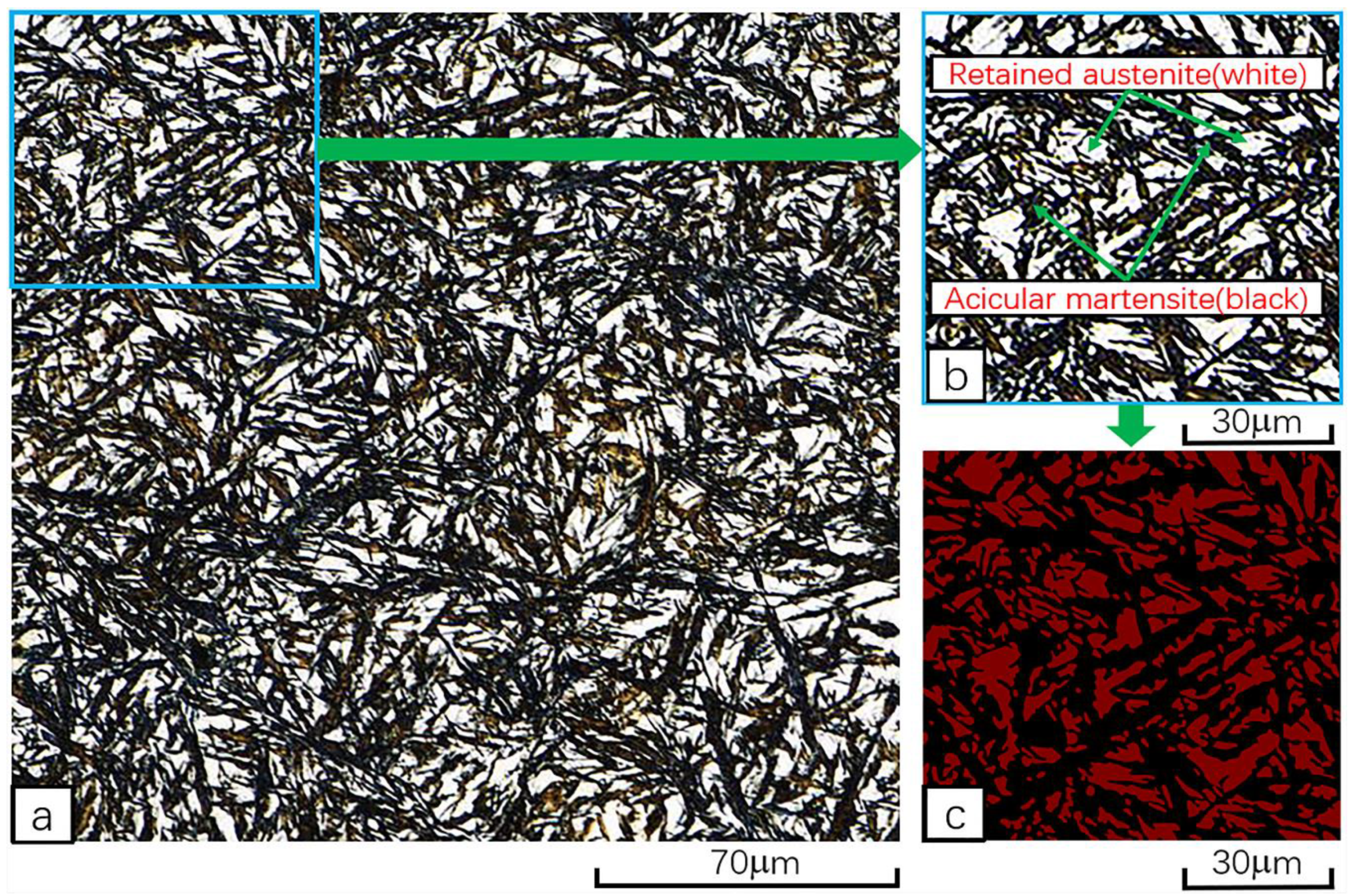
2.2. Optical Micrograph

Microstructure samples with a thickness of 10 mm were obtained along the cross-section of the raw material bar by wire cutting. The observation surface was first ground with metallographic water sandpaper (#800 to #5000) and then polished on a metallographic polishing machine with a 0.5 μm diamond polishing agent. Then, the polished sample was placed in alcohol for ultrasonic cleaning and dried with a hairdryer after cleaning, as shown in Figure 1, which depicts the microstructure of a sample from the surface to the core. This experiment used five processes and obtained 1200 microstructure photos for SegModel-MOS training and testing.

2.3. Residual Stress and Residual Austenite Testing

The electrochemical method was used to strip the sample; then, the residual stress of each layer was tested using the Italian GNR STRESS-X residual stress analyzer. The quenching stress field had the characteristic of the stress gradient of the near-surface layer being relatively large. Therefore, when designing the stripping thicknesses, the stripping thickness of the near-surface layer was small. As the depth increased, the stripping thickness gradually increased. After measuring the residual stress of each layer, the residual austenite was measured, and a dial gauge-height meter was used to measure the height of the test before and after delamination.

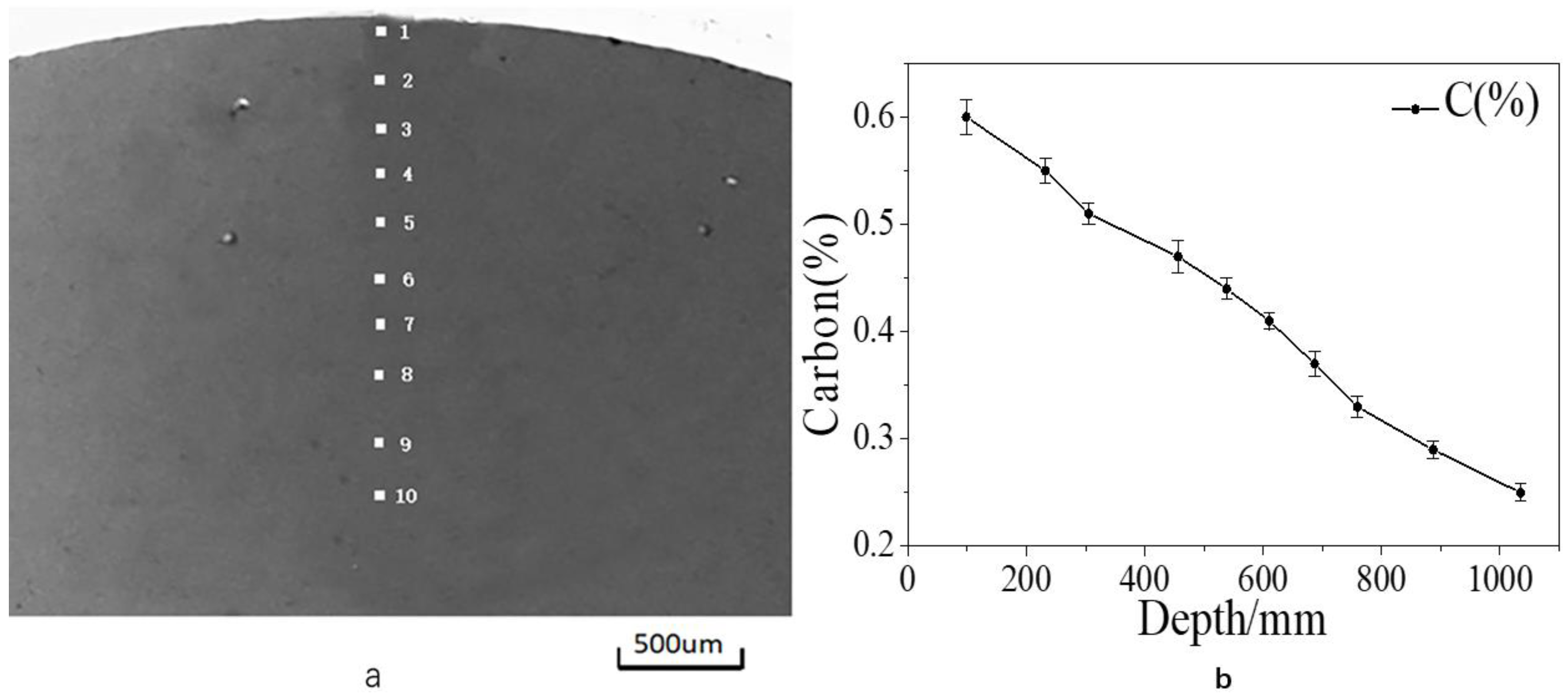
2.4. Carburizing Layer Carbon Content Measurement

Bedroom machine tools were used to strip the carburized parts; each stripping thickness was the same as the residual stress stripping thickness. Then, the JS-HW2000A high-frequency infrared carbon and sulfur analyzer was used to measure the carbon content of each layer of metal powder. The measurement error of the analyzer is 0.0001–0.05%, and it measures the gradient change in the carbon content of the carburized layer. Figure 2 presents some of the data measurement points and the corresponding carbon content. During the carburizing process, a high concentration of activated carbon atoms forms on the surface of the workpiece, is adsorbed into the surface of the workpiece, and then diffuses to the core of the workpiece, gradually forming a carbon concentration gradient.

3. Method

3.1. Data Processing

1)

Data processing: The image resolutions in the dataset were not uniform; their lengths and widths ranged between 200 and 550 pixels. The minibatch training method requires the input image size to be consistent; therefore, the input images needed to be cropped. First, the long side of the image was left unchanged, and padding was added to both sides of the image (pixels with 0 values were added). Then, nearest-neighbor interpolation was used to scale the image to 384 × 384. This processing step not only yields input images of the same size but also ensures that the aspect ratio of the original image is unchanged and that the structural information of the target is retained to the utmost degree. Although this method adds considerable padding, the network treats it as redundant information; thus, the added pixels are not used during training. It should be noted that the original images were also cropped, and the ground truth labels of the image needed to be cropped accordingly.

2)

Data enhancement: Although the CNN greatly reduces the number of parameters that must be learned due to its weight sharing function, the number of parameters in the network still reaches hundreds of millions. This enormous number of parameters requires large amounts of data; training from too few data samples will lead to insufficient network generalizability, overfitting, and other problems. To enrich the data samples, the following data augmentation operations were performed on the training set: (1) horizontal flipping: during the training process, each iteration flipped the image left or right at a probability of 0.5; (2) panning: the input image was randomly translated horizontally and vertically within a range of 20 pixels; (3) rotation: the image was rotated randomly at an angle, ranging from −20 to 20°; (4) noise: Gaussian random noise with a mean of 0.2 and a variance of 0.3 was added to the image.

3)

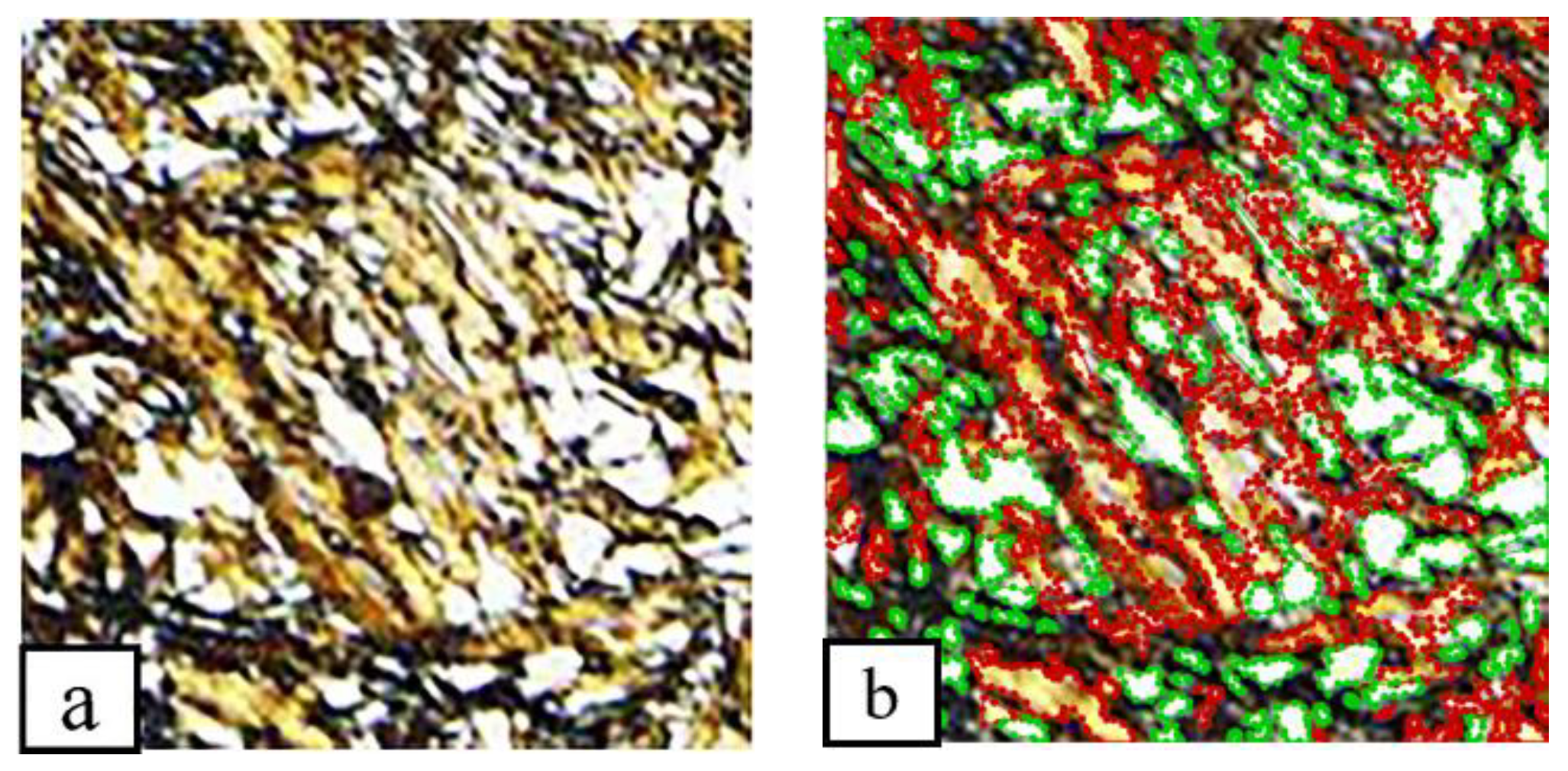
Data set labeling and production: To identify steel microstructures, it was first necessary to use a labeling tool such as LabelMe to manually mark the positions of acicular martensite, retained austenite, and lath martensite in the original image data, as shown in Figure 3. A total of 1200 material microstructure pictures were marked. During the marking process, the microstructure label information of the microstructure was stored in an XML file format that included the path and file name of the original picture, the size of the picture, the label names “Acicular martensite”, “Retained austenite”, and “Batten martensite” (the same categories as in SegModel-MOS training) and the positional information of each label box. The file format complied with the PASCAL VOC data format, which includes two main folders: Annotations and JPEGImages. The former is mainly used to store the XML files containing the tags, and the latter is used to store the original image data. Finally, the PASCAL VOC data format was converted into a TFRecord data file, which is a binary file that combines images and labels together to make better use of the memory in TensorFlow [25] and achieve fast copy, move, store, read, and other data operations.

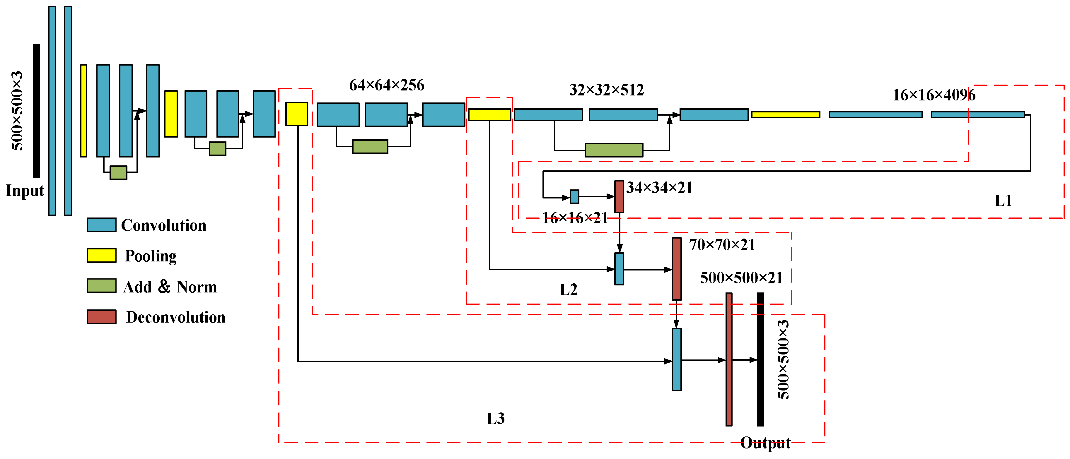
3.2. The Structure of the Material Organization Structure Segmentation Model (SegModel-MOS)

Semantic segmentation is an important field in computer vision that refers to identifying image content at the pixel level by marking the object category to which each pixel in the image belongs. Common applications include self-driving cars [26,27,28,29,30] and medical image diagnosis [31,32,33]. In 2014, Long and others at the University of California, Berkeley proposed a fully convolutional network (FCN) [34] that allowed a CNN to perform dense pixel prediction without a fully connected layer, which popularized CNNs. The easiest way to build a neural network architecture for semantic segmentation tasks is to simply stack multiple convolutional layers (of the same sizes to retain the required dimensions) and output the final segmentation graph. This approach learns a mapping from the input image to its corresponding segmentation through the continuous transformation of feature maps.

In this study, a segmentation model for the material organization structure (SegModel-MOS) was built on AlexNet, as shown in Figure 4. Our goal was to segment the content types in the SEM image rather than classify the image. Thus, we removed the last fully connected layer and the last convolutional layer of the AlexNet network and added residual blocks between the convolutional layers of the AlexNet to prevent overfitting. The deconvolution operation was performed in the remaining layers of the network, as shown in Figure 4. First, a convolution layer was added based on L1, and then bilinear interpolation deconvolution was performed with a step size of 2 on the output of the convolution layer. Another convolution layer was then added based on L2. Then, the output of the convolution layer and the deconvolution result of L1 were added and fused, and bilinear interpolation deconvolution with a step size of 2 was performed. Finally, a convolutional layer was added based on L3. The output result of this convolutional layer was added and fused with the deconvolution result of L2, and then a bilinear interpolation deconvolution layer with a step size of 8 was applied. After each convolution layer, a linear rectifier unit (ReLU) was used as the activation function.

Table 2. SegModel-MOS parameters.

	Layer	Input Shape	Filter	Kernel Size	Stride	Output Shape
L1	Conv		[batch, 14, 14, 1024]		21	(3, 3, 1024)	(1,1)	[batch, 16, 16, 21]
	Deconv		[batch, 16, 16, 21]		21	(3, 3, 21)	(2,2)	[batch, 34, 34, 21]
L2	Conv		[batch, 32, 32, 512]		21	(3, 3, 512)	(1,1)	[batch, 34, 34, 21]
	Deconv		[batch, 34, 34, 21]		21	(3, 3, 21)	(2,2)	[batch, 70, 70, 21]
L3	Conv		[batch, 64, 64, 256]		21	(3, 3, 256)	(1,1)	[batch, 70, 70, 21]
	Deconv		[batch, 70, 70, 21]		21	(3, 3, 21)	(8,8)	[batch, 500, 500, 21]

lists some of the parameters of the SegModel-MOS network.

3.3. SegModel-MOS Training

(1) Model training: The SegModel-MOS model was first trained on the PASCAL VOC2012 [35] dataset. After the model had been trained for 800 steps, its verification set accuracy was 85%. At that point, the model began to overfit, and the validation set accuracy underwent a downward trend. After the model has been trained to 3000 steps, the accuracy of the model test was 80%. During the model training process, in this study, we saved the trained model at each step. Using an early termination criterion [36], we selected the model version before it began to overfit (that is, the version where the model was trained for 800 steps) and conducted migration learning using our own method. The enhanced data of the acquired microstructure map were used to train the model. Taking 80% of the enhanced dataset as training data and 20% as test data, the model was trained and validated numerous times, and the neural network hyperparameter learning rate, optimization algorithms, and batch size were searched. First, the initial value for each hyperparameter was set based on empirical intuition; then, a greedy algorithm was used to gradually adjust each hyperparameter. Finally, the network weights with the best performances on the test set were identified, as shown in

Table 3. Test result record during model training.

Optimization Algorithms	Learning Rate	Batch Size	Test Set Ratio	Test Set Accuracy
Adam	0.1	4	20%	93.7%
	0.01	4	20%	91.6%
	0.001	4	20%	92.8%
	0.0001	4	20%	91.0%
	0.01	8	20%	94.7%
	0.01	16	20%	93.9%
	0.01	32	20%	95.2%
Momentum	0.1	4	20%	92.4%
	0.01	4	20%	92.9%
	0.001	4	20%	93.9%
	0.0001	4	20%	93.7%
	0.01	8	20%	91.1%
	0.01	16	20%	92.7%
	0.01	32	20%	89.3%

below. From Table 3, the best hyperparameters for the model are as follows: the batch size of 32, the learning rate of 0.01, and the use of the Adam optimization algorithm.

(2) Network model improvements: To enable the SegModel-MOS model to identify and classify the material microstructures and improve the classification accuracy, this study improved the network based on both the initial dataset and the network trained via migration learning. Based on the average size of the microscope images, we changed the input image size of the network to 256 × 256 × 3. After this change, the microscope images were similar in size to their manual enlargements. This change not only improved the quality of manual marking but also made local features easier to identify and improved the network feature extraction effect. In addition, the color category of the dataset in this article contained only three colors: black, white, and yellow. Thus, the output category of the softmax layer of the last layer was changed to 3.

(3) Network improvement based on transfer learning: When the raw PASCAL VOC2012 data were used to train the initial SegModel-MOS model, the optimal hyperparameters were found, and the optimal recognition model obtained was transferred to the microscopic image recognition task. During the migration process, the top part of the network (including the global average pooling layer and logistic regression layer of the last layer) was removed, and feature migration was performed. Based on the task differences, the top-level part still used a random initialization strategy to adapt it to the color classification task after sufficient training. Then, based on the network structure, the features in some layers were frozen, and the remaining layers were fine-tuned to ensure high accuracy while reducing the number of network parameters and model complexity, as shown in Figure 5, which depicts a model segmentation comparison.

4. Results and Discussion

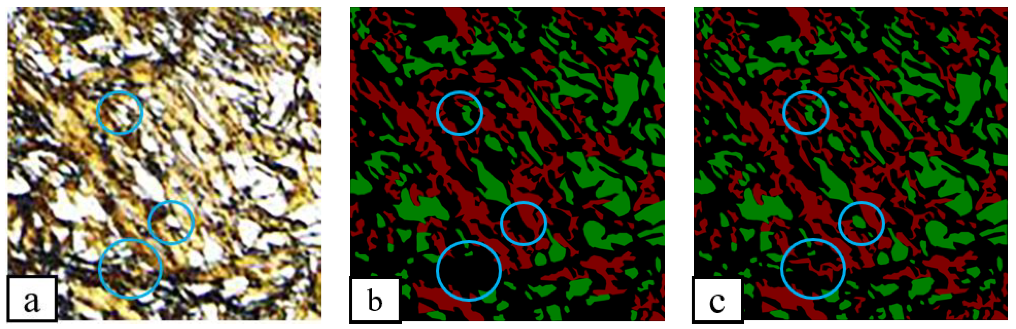
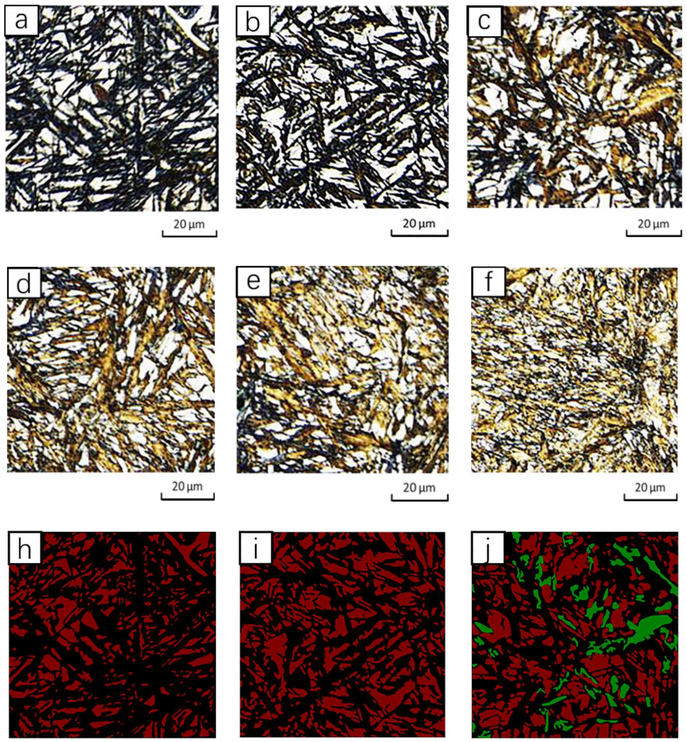
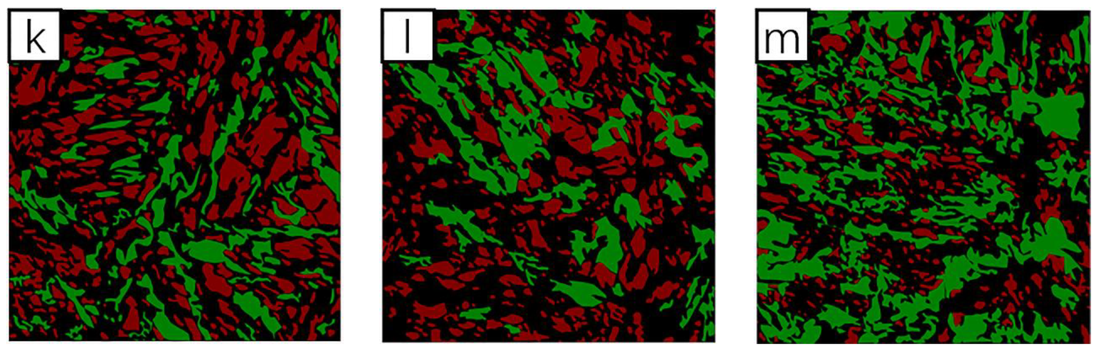
4.1. Picture Segmentation

In the use phase of SegModel-MOS, each image must be divided into nine parts for segmentation, as shown in Figure 6, to maintain the consistency between the size of the input data and that of the training data. This process also increases the segmentation accuracy of SegModel-MOS.

Figure 7 contains a partial subset of each sample from the surface to the centripetal part and shows the segmentation effect of SegModel-MOS on the image. In the image, black represents acicular martensite, white is retained austenite, and yellow denotes lath martensite. After carburizing and quenching, the heart structure is a slat-like distribution of low-carbon martensite, which has high strength and good impact toughness. After tempering the sample at 200 °C for 2 h, the martensite in the surface carburized layer is easily eroded and blackened. In contrast, the retained austenite does not erode easily and appears white. Therefore, in the daily metallographic examination, it is generally believed that the white areas crossed by the martensite needles retain austenite. However, it should be noted that the white areas retain austenite with a small amount of carbide on the surface, which is also white.

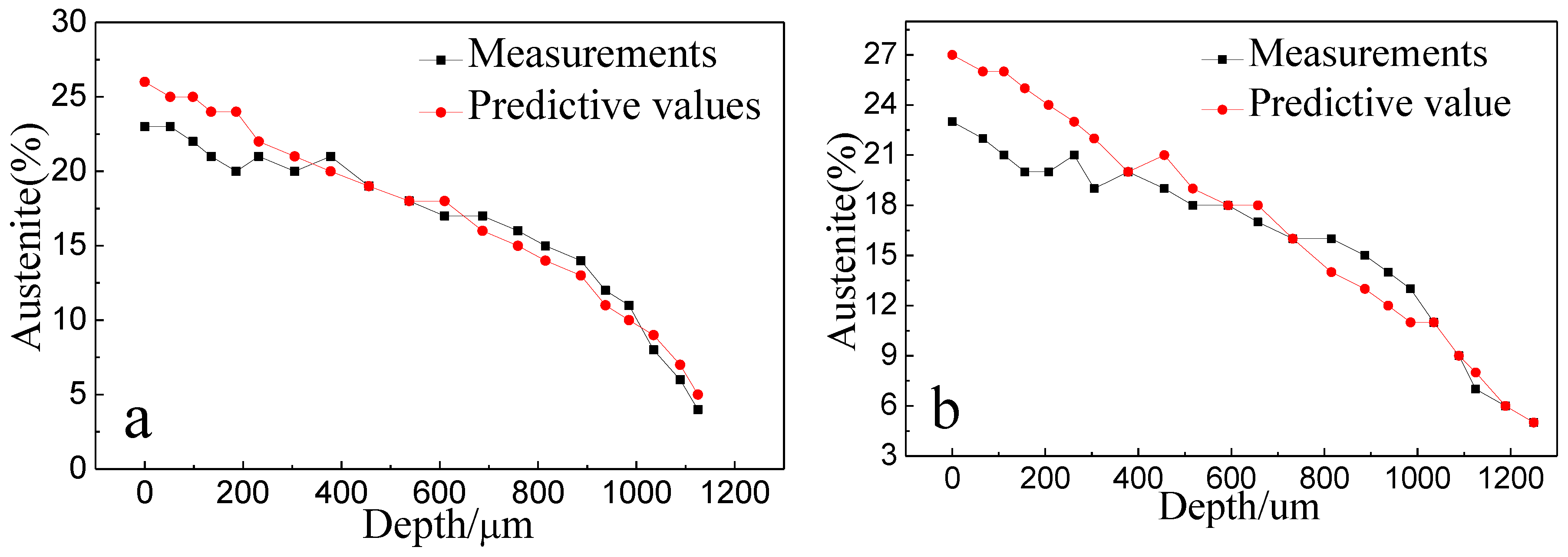
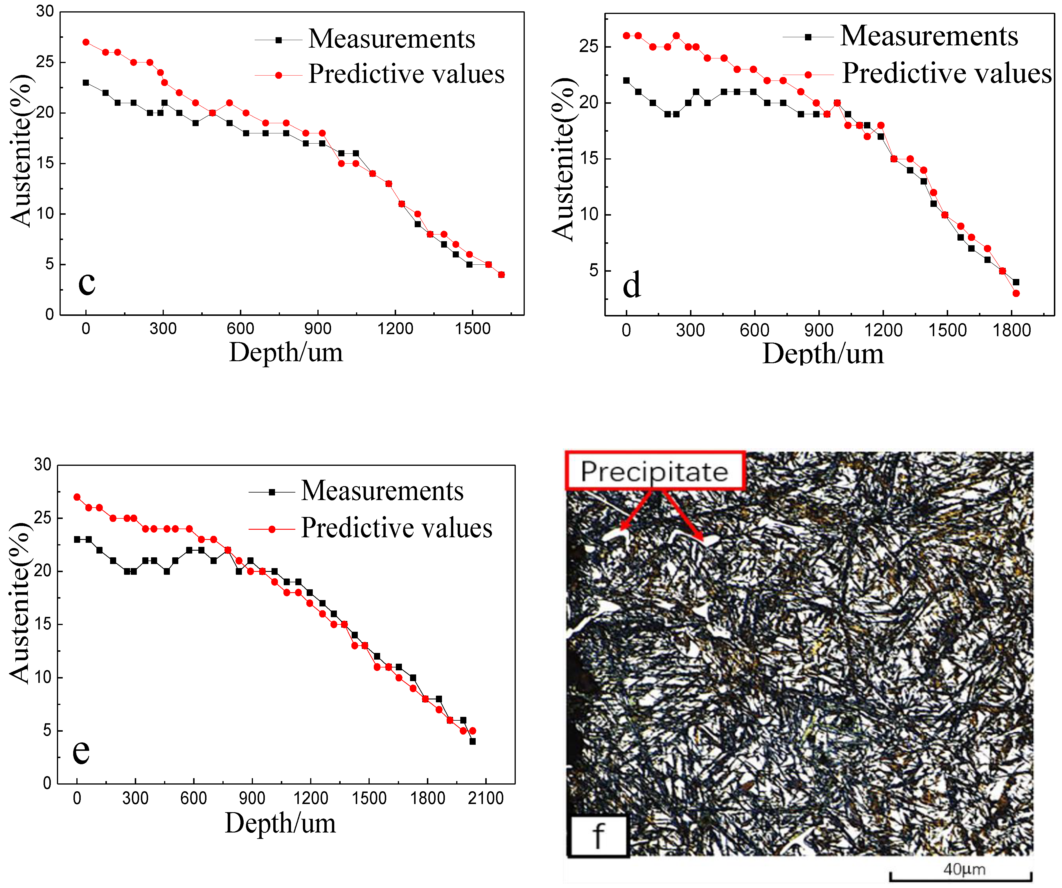
4.2. Comparison of Measured and Predicted Values of Retained Austenite

To verify the effect of metallographic image segmentation, the residual austenite was measured with an Italian GNR STRESS-X residual stress analyzer, and the results were compared with the predicted values. Figure 8a,b presents the carburized layer at 0–200 μm, Figure 8c,d shows the carburized layer at 0–300 μm, and Figure 8e shows the carburized layer at 0–400 μm with the residual austenite. The differences between the measured and predicted values range between approximately 1% and 3.5%. This finding is attributed to the fact that in a carburized sample, the carbon content of the surface layer is a hypereutectoid carburized area, and white carbide will appear mixed between the needle-shaped martensite and residual austenite, as shown in Figure 8f. The precipitated carbides are observed, and the precipitated carbides on the surface layer are calculated by image segmentation to account for 1%–3.5%. To eliminate the influence of surface carbides, Figure 8a–e demonstrates that deep learning exhibits a high accuracy rate for image segmentation in the areas after the subsurface of the sample, and the error between the measured and predicted values of residual austenite is very small. An increase in the carbon content in the steel reduces the temperature at which martensite begins to form, leading to austenite stabilization and increasing the amount of retained austenite. The carbon content of the carburized layer gradually decreases from the surface to the center; therefore, the amount of retained austenite in Figure 8 gradually decreases from the surface to the center.

4.3. Prediction Results and Analysis of Residual Stress

4.3.1. Residual Stress Prediction Principle

Residual stress is caused by stresses that include thermal and phase transition stresses. There are two explanations for the residual stress in the quenched part. One explanation involves the thermal stress caused by the temperature difference between the surface and the core of the quenched part, and the second explanation involves the structural stress caused by the phase change and the integrated value. However, because the surface of the sample is carburized, the carbon content of the carburized layer changes only gradually; the carbon content is high at the surface but low in the core. The change in carbon content plays a leading role in the residual stress value. Therefore, the residual stress is mainly attributable to the cooling process, and the volume expansion of the martensite transformation varies due to the differences in carbon content in different parts of the surface layer. In addition, after quenching, the surface morphologies of the martensite and transition layers are inconsistent and form a structural gradient. The carburized surface layer consists of acicular martensite and residual austenite, the transition layer consists of acicular martensite and batten martensite plus some residual austenite, and the core consists of batten martensite and a small number of residual austenite bodies. After the martensite transformation occurs during quenching, the martensite solid-solution carbon content in the surface carburized layer is high, resulting in increased hardness compared with the core after quenching and the formation of a hardness gradient. When the high carbon content of the surface layer is martensitic, it undergoes a greater volume expansion than that of the low-carbon-content core. Thus, a residual compressive stress gradient is formed. Therefore, the carbon content and microstructure can be used to predict the residual stress. This article trained a model using 1200 sets of data from Process 1 to Process 5 ranging from the surface to the heart. Some of these data are shown in

Table 4. 23CrNi3Mo carburized steel Process 1 data.

Depth (um)	C (%)	Acicular Martensite (%)	Retained Austenite (%)	Lath Martensite (%)	Residual Stress (MPa)
98	0.60	0.78	0.22	0	−334
232	0.56	0.79	0.21	0	−377
305	0.53	0.80	0.20	0	−343
456	0.48	0.76	0.19	0.05	−242
538	0.46	0.69	0.18	0.13	−210
610	0.43	0.62	0.17	0.21	−185
687	0.40	0.54	0.17	0.29	−161
759	0.37	0.50	0.16	0.34	−155
887	0.31	0.38	0.14	0.48	−125
985	0.27	0.28	0.11	0.61	−77
1089	0.23	0.15	0.06	0.79	−69

. Each dataset is a 256 × 256 pixel picture; based on deep learning image segmentation, each picture is analyzed for acicular martensite, retained austenite, lath martensite, and the residual stress at the corresponding points.

4.3.2. Prediction of Residual Stress Based on the SVM Model

First, the data were preprocessed and normalized to eliminate dimensional differences between the parameter ranges and improve the accuracy of the SVM model:

$$Z=\frac{X-\mu }{\sigma }$$

(1)

where Z denotes the normalized data, X is the original data from the datasets, and μ and σ represent the mean and standard deviation of the original data, respectively.

The use of kernel functions to embed samples into the high-dimensional feature space is crucial to constructing a generalizable SVM model. This paper adopted a radial basis function (RBF) kernel suitable for nonlinear problems. The generalizability of the SVM based on RBF is controlled by a key parameter, namely C [37], which is the penalty parameter in the SVM objective function and is set to a constant greater than zero. Setting parameter C to a too-large value leads to overfitting, while setting C to a too-small value leads to underfitting. The search process to find the optimal parameters was conducted for 500 generations, and the search range for the parameter C was 0–500.

The dataset obtained in the experiment contained a total of only 1200 samples. Because the number of samples in the current work was quite limited, the performance of the trained model varied substantially based on the division of the training and test sets. In addition, a random division of the dataset can easily lead to unbalanced data distributions and inaccurate model performance evaluations. Therefore, this study used 10-fold cross-validation to evaluate model generalizability. We adopted R-squared (R²) and mean absolute error (MAE) as the evaluation indicators:

$${{\displaystyle R}}^2=1-\frac{{\displaystyle {\sum }_{i=1}^m{{\displaystyle ({{\displaystyle y}}_i-{{\displaystyle \widehat{y}}}_i)}}^2}}{{\displaystyle {\sum }_{i=1}^m{{\displaystyle ({{\displaystyle y}}_i-{{\displaystyle \overline{y}}}_i)}}^2}}$$

(2)

$$MAE=\frac{1}{m}{\displaystyle \sum _{i=1}^m\left|{{\displaystyle y}}_i-{{\displaystyle \widehat{y}}}_i\right|}$$

(3)

where m is the number of samples, ${{\displaystyle y}}_i$ is the true value, ${{\displaystyle \widehat{y}}}_i$ is the predicted value, ${{\displaystyle \overline{y}}}_i$ is the average of the real labels of m samples, and $i$ is the sample label.

To further verify the model prediction effect, we introduced a decision tree model to predict the residual stress. First, the hyperparameters of the model were optimized; then, the same 5-fold cross-validation approach was used to compare the measured and predicted residual stress values in the test dataset with the fitted straight line shown in Figure 9.

Figure 9 shows the 5-fold cross-validation results for the SVM and decision tree (DT) models. Most of the points in the test dataset lie either on or very close to the straight line with a slope of 1, which strongly indicates that most of the predicted values are in good agreement with the experimental values. This finding demonstrates that both the SVM and DT models have good generalizability and achieve high prediction accuracy. Figure 9 shows that the values of SVM and DT model R² are 0.975 and 0.953, respectively, and their MAE values are 7.52 MPa and 12.45 MPa, respectively. The results predicted by the SVM model are presented in Figure 9a, where the absolute error between the experimental and predicted values of 178 out of 240 samples is within a 10.0 MPa range, and the maximum absolute error is 15.5 MPa. The results predicted by the DT model are presented in Figure 9b, where the absolute error between the experimental and predicted values of 132 out of 240 samples is within 10.0 MPa, and the maximum absolute error is 25.5 MPa. In summary, the SVM and DT models exhibit minimal deviations between the predicted and measured values of residual stress; however, the R² and MAE results of the SVM model are significantly better than those of the DT model, indicating that the SVM model is more suitable for the entire dataset.

4.4. Discussion

In this study, the SegModel-MOS network was used to segment optical microstructure images, and the SVM algorithm was used to predict the residual stress, constituting a new method for measuring residual stress in the future. However, the mapping relationship between the optical image and the residual stress was not established directly, mainly because the data in the optical image were limited, and the training model could easily overfit. In the future, we will seek to establish the mapping relationship between the optical images and residual stress directly. This initial network model has high requirements for the input images, and its computational burden is relatively high; however, the model can appropriately reduce the pixels, increase the number of residual network layers, and reduce the amount of calculation. In addition, the carbon content and microstructure of steel not only are related to the residual stress but also exhibit a strong correlation with the mechanical properties. The mechanical properties of alloy steel mainly depend on the carbon content, alloying elements, and heat treatment process. Therefore, we propose a deep learning model to predict the mechanical properties of alloy steel and improve the fatigue life of the samples. The SVM model uses carbon content and microstructure to predict residual stress with high accuracy, while the SegModel-MOS model uses migration learning to segment the microstructure of carburized steel and then uses machine learning to predict the residual stress. This approach can also be used to analyze the performance of other carburized steels, providing a new method for use in carburized steel performance research.

5. Conclusions

1)

This paper proposes a new method to predict residual stress using a semantic segmentation model (SegModel-MOS). After training on the PASCAL VOC2012 dataset, the network was trained on optical microscope images to achieve precise segmentation, revealing the residual austenite and measuring the content percentages. The results demonstrate that the accuracy of the model’s microstructure segmentation reaches 95.2%.

2)

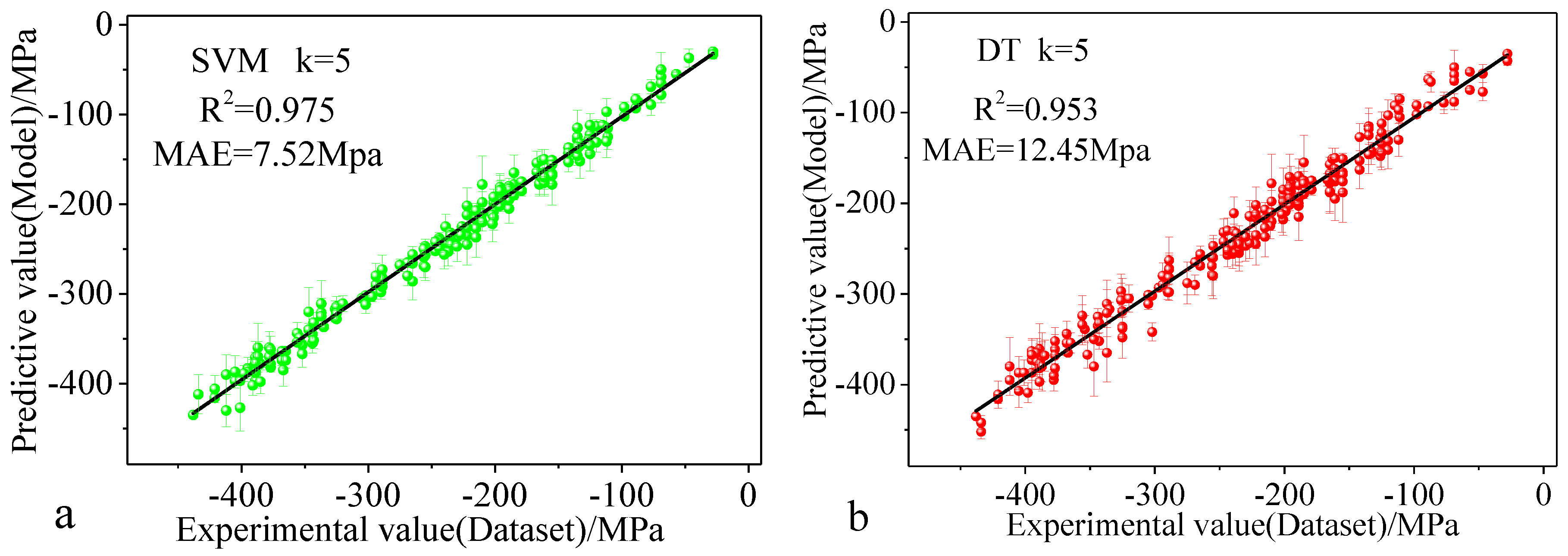
SVM and decision tree algorithms were used to build a mapping relationship between the carbon content, microstructure, and residual stress of steel. The SVM and DT models used 5-fold cross-validation to improve model generalizability, achieving final residual stress prediction R² values of 0.975 and 0.953 and the MAE values of 7.52 MPa and 12.45 MPa, respectively. The SVM model performed significantly better than the DT model. This finding demonstrates that carbon content and microstructure exhibit high accuracy and generalization ability for predicting residual stress. This method can also be used to predict the residual stress of other carburized steels; thus, it constitutes a new approach to residual stress measurement.

References

1. Farfán, C.; Rubio-González, T.; Cervantes-Hernández, T.; Mesmacque, G. High cycle fatigue, low cycle fatigue and failure modes of a carburized steel. Int. J. Fatigue 2004, 26, 673–678. [Google Scholar]
2. Nehila, A.; Li, W.; Gao, N. Very high cycle fatigue of surface carburized CrNi steel at variable stress ratio: Failure analysis and life prediction. Int. J. Fatigue 2018, 111, 112–123. [Google Scholar] [CrossRef]
3. Yanzhi, L.; Chunzhi, L.I.; Xudong, L.I. Surface Integrity Characteristics and Fatigue Failure Mechanism of Carburized M50NiL Steel. J. Aeronaut. Mater. 2017, 37, 25–33. [Google Scholar]
4. Deng, H.; Liu, Q.; Liu, H. Long-Life Fatigue of Carburized 12Cr2Ni Alloy Steel: Evaluation of Failure Characteristic and Prediction of Fatigue Strength. Metals 2018, 8, 1006. [Google Scholar] [CrossRef] [Green Version]
5. Tremarin, R.C.; Pravia, Z.M.C. Analysis of the Influence of Residual Stress on Fatigue Life of Welded Joints. Latin Am. J. Solids Struct. 2020, 17. [Google Scholar] [CrossRef]
6. Li, W.; Sun, Z.; Deng, H. Interior crack initiation and growth behaviors and life prediction of a carburized gear steel under high cycle fatigue and very high cycle fatigue. J. Mater. Res. 2015, 30, 2247–2257. [Google Scholar] [CrossRef]
7. Shen, C.; Wang, C.; Wei, X. Physical metallurgy-guided machine learning and artificial intelligent design of ultrahigh-strength stainless steel. Acta Mater. 2019, 179, 201–214. [Google Scholar] [CrossRef]
8. Ampazis, N.; Alexopoulos, N.D. Prediction of aircraft aluminum alloys tensile mechanical properties degradation using support vector machines//Artificial Intelligence: Theories, Models and Applications. In Proceedings of the 6th Hellenic Conference on AI, SETN 2010, Athens, Greece, 4–7 May 2010; Springer: Berlin/Heidelberg, Germany, 2010; Volume 9, pp. 115–133. [Google Scholar]
9. Aarnts, M.P. Microstructural Quantification of Multi-Phase Steels (Micro-Quant); European Commission: Luxembourg, 2011. [Google Scholar]
10. Burikova, K.; Rosenberg, G. Quantification of Microstructural Parameter Ferritic-Martensite Dual Phase Steel by Image Analysis. Metal 2009, 5, 19–21. [Google Scholar]
11. Dengiz, O.; Smith, A.E.; Nettleship, I. Grain boundary detection in microstructure images using computational intelligence. Comput. Ind. 2005, 56, 854–866. [Google Scholar] [CrossRef]
12. Dutta, S. Characterization of micrographs and fractographs of Cu-strengthened HSLA steel using image texture analysis. Measurement 2014, 47, 130–144. [Google Scholar] [CrossRef]
13. Komenda, J. Automatic recognition of complex microstructures using the Image Classifier. Mater. Charact. 2001, 46, 87–92. [Google Scholar] [CrossRef]
14. De Cost, B.L.; Holm, E.A. A computer vision approach for automated analysis and classification of microstructural image data. Comput. Mater. Sci. 2015, 110, 126–133. [Google Scholar] [CrossRef] [Green Version]
15. Adachi, Y.; Taguchi, M.; Hirokawa, S. Microstructure Recognition by Deep Learning. Tetsu Hagané 2016, 102, 62–69. [Google Scholar]
16. Masci, J.; Meier, U.; Ciresan, D.; Schmidhuber, J.; Fricout, G. Steel Defect Classification with Max-pooling Convolutional Neural Networks. In Proceedings of the 2012 International Joint Conference on Neural Networks (IJCNN), Brisbane, QLD, Australia, 10–15 June 2012. [Google Scholar]
17. Bai, L.; Velichko, A.; Drinkwater, B.W. Characterization of defects using ultrasonic arrays: A dynamic classifier approach. IEEE Trans. Ultrason. Ferroelectr. Freq. Control 2015, 62, 2146–2160. [Google Scholar] [CrossRef]
18. Bulgarevich, D.S.; Tsukamoto, S.; Kasuya, T. Pattern recognition with machine learning on optical microscopy images of typical metallurgical microstructures. Sci. Rep. 2018, 8, 2078. [Google Scholar] [CrossRef] [PubMed]
19. Azimi, S.M.; Britz, D.; Engstler, M. Advanced Steel Microstructural Classification by Deep Learning. Methods Rep. 2018, 8, 2128. [Google Scholar] [CrossRef]
20. Wang, S.C.; Kao, P.W. The effect of alloying elements on the structure and mechanical properties of ultralow carbon bainitic steels. J. Mater. Sci. 1993, 28, 5169–5175. [Google Scholar] [CrossRef]
21. Wei, X.; Yang, F.; Wu, C. Deep residual networks of residual networks for image super-resolution. Lidar Imaging Detect. Target Recognit. 2017, 75, 1–10. [Google Scholar]
22. Northwood, D.O.; He, L.; Boyle, E. Retained Austenite Residual Stress—Distortion Relationships in Carburized SAE 6820 Steel. Mater. Sci. Forum 2007, 539–543, 4464–4469. [Google Scholar] [CrossRef]
23. Deng, H.L.; Liu, H.Q.; Liu, Q.C. Fatigue strength prediction of carburized 12Cr steel alloy: Effects of evaluation of maximum crack sizes and residual stress distribution. Fatigue Fract. Eng. Mater. Struct. 2020, 43, 342–354. [Google Scholar] [CrossRef]
24. Qing, Y.X.; Yu, K.G. Effect of carburization on residual stress field of 20CrMnTi specimen and its numerical simulation. Mater. Sci. Eng. A 2005, 392, 240–247. [Google Scholar]
25. Abadi, M.; Agarwal, A.; Barham, P. TensorFlow: Large-Scale Machine Learning on Heterogeneous Distributed Systems. arXiv 2016, arXiv:1603.04467. [Google Scholar]
26. Sviatov, K.; Miheev, A.; Kanin, D. Scenes Segmentation in Self-driving Car Navigation System Using Neural Network Models with Attention. In International Conference on Computational Science and Its Applications; Springer: Cham, Switzerland, 2019. [Google Scholar]
27. Zhang, Y.; Wang, J.; Wang, X. Road-Segmentation-Based Curb Detection Method for Self-Driving via a 3D-LiDAR Sensor. IEEE Trans. Intell. Transp. Syst. 2018, 19, 3981–3991. [Google Scholar] [CrossRef]
28. Zheng, N. A Co-Point Mapping-Based Approach to Drivable Area Detection for Self-Driving Cars. Engineering 2018, 4, 479–490. [Google Scholar]
29. Treml, M.; José, A.-M.; Unterthiner, T. Speeding up Semantic Segmentation for Autonomous Driving. NIPS Workshop-MLITS 2016, 89, 66–84. [Google Scholar]
30. Yunyan, W.; Lengkun, L.; Zhigang, Z. Road scene segmentation based on KSW and FCNN. J. Image Graph. 2019. [Google Scholar] [CrossRef]
31. Bruijne, M.D. Machine learning approaches in medical image analysis: From detection to diagnosis. Med Image Anal. 2016, 33, 218–236. [Google Scholar] [CrossRef] [Green Version]
32. Xue, F.F.; Peng, J.; Wang, R. Improving Robustness of Medical Image Diagnosis with Denoising Convolutional Neural Networks. In International Conference on Medical Image Computing and Computer-Assisted Intervention; Springer: Cham, Switzerland, 2019. [Google Scholar]
33. Youping, Z.; Radiology, D.O. Rational application of medical imaging technology in medical image diagnosis. J. Imaging Res. Med. Appl. 2019, 4, 126–138. [Google Scholar]
34. Long, J.; Shelhamer, E.; Darrell, T. Fully Convolutional Networks for Semantic Segmentation. IEEE Trans. Pattern Anal. Mach. Intell. 2015, 39, 640–651. [Google Scholar]
35. Shetty, S. Application of Convolutional Neural Network for Image Classification on Pascal VOC Challenge 2012 dataset. arXiv 2016, arXiv:1607.03785. [Google Scholar]
36. Yao, Y.; Rosasco, L.; Caponnetto, A. On Early Stopping in Gradient Descent Learning. Constr. Approx. 2007, 26, 289–315. [Google Scholar] [CrossRef]
37. Dyson, D.J.; Keown, S.R. A study of precipitation in a 12 %Cr-Co-Mo steel. Acta Met. 1969, 17, 1095–1107. [Google Scholar] [CrossRef]
Figure 1. Optical micrographs from the surface to the heart of the Process 1 sample: (a) carburized surface layer; (b) transition layer; (c) black (acicular martensite); white (retained austenite); (d) yellow (lath martensite).
Applsci 10 07759 g001
Figure 2. (a) The measured points in sequence; (b) the change in the surface carbon content.
Applsci 10 07759 g002
Figure 3. Manual labeling of microstructure pictures: (a) original picture; (b) manually marked picture (red marked as lath martensite, green marked as retained austenite, black (not marked) as acicular martensite).
Applsci 10 07759 g003
Figure 4. Material organization structure segmentation model (SegModel-MOS) architecture.
Applsci 10 07759 g004
Figure 5. (a) Original image; (b) segmented image without the improved network model; (c) segmented image with the improved network model.
Applsci 10 07759 g005
Figure 6. Splitting method when inputting microstructure images into SegModel-MOS, (a) Original Picture; (b) Crop picture; (c) segmentation Picture.
Applsci 10 07759 g006
Figure 7. The segmentation effect of SegModel-MOS: Acicular martensite (black), retained austenite (red), and lath martensite (green). (af), the images range from the surface of the carburized layer to the core; (hm), SegModel-MOS model segmentation picture.
Applsci 10 07759 g007aApplsci 10 07759 g007b
Figure 8. (ae), comparison of the retained austenite measurements and the predicted values after deep learning identification; (f) Surface microstructure picture.
Applsci 10 07759 g008aApplsci 10 07759 g008b
Figure 9. Comparison of the predicted residual stress values of support vector machine (SVM) and decision tree (DT) models with the experimental values: (a) SVM model 5-fold cross-validation results; (b) DT model 5-fold cross-validation results.
Applsci 10 07759 g009