Article

Design of a Low-complexity Graph-Based Motion-Planning Algorithm for Autonomous Vehicles

1
Department of Control for Transportation and Vehicle Systems, Budapest University of Technology and Economics, Stoczek u. 2, H-1111 Budapest, Hungary
2
Systems and Control Laboratory, SZTAKI Institute for Computer Science and Control, Kende u. 13-17, H-1111 Budapest, Hungary
*
Author to whom correspondence should be addressed.
Appl. Sci. 2020, 10(21), 7716; https://doi.org/10.3390/app10217716
Submission received: 1 September 2020 / Revised: 13 October 2020 / Accepted: 28 October 2020 / Published: 31 October 2020
(This article belongs to the Special Issue Connected Automated Vehicles)

Abstract

:
In the development of autonomous vehicles, the design of real-time motion-planning is a crucial problem. The computation of the vehicle trajectory requires the consideration of safety, dynamic and comfort aspects. Moreover, the prediction of the vehicle motion in the surroundings and the real-time planning of the autonomous vehicle trajectory can be complex tasks. The goal of this paper is to present low-complexity motion-planning for overtaking scenarios in parallel traffic. The developed method is based on the generation of a graph, which contains feasible vehicle trajectories. The reduction of the complexity in the real-time computation is achieved through the reduction of the graph with clustering. In the motion-planning algorithm, the predicted motion of the surrounding vehicles is taken into consideration. The prediction algorithm is based on density functions of the surrounding vehicle motion, which are developed through real measurements. The resulted motion-planning algorithm is able to guarantee a safe and comfortable trajectory for the autonomous vehicle. The effectiveness of the method is illustrated through simulation examples using a high-fidelity vehicle dynamic simulator.

1. Introduction and Motivation

Nowadays, one of the main challenges for the automotive industry is the development of autonomous vehicles, which involves the solution of several problems, e.g., motion-planning, control, design and implementation of the algorithms. In everyday traffic, motion-planning functionality is crucial, in which several requirements must be simultaneously guaranteed, i.e., the vehicle trajectory must be dynamically feasible, safe and comfortable. There are existing technologies for this problem, although they only provide suggestions for the driver during the maneuver [1,2]. The overtaking maneuvers are especially dangerous since the motion of other participants must be predicted, in order to guarantee the collision-free trajectory. Furthermore, there can be overtaking situations when a feasible trajectory cannot be planned between the initial and the target state of the vehicle. The stability and the trajectory tracking problems of the vehicles under varying circumstances must be solved, which requires the design of robust control systems. In the future, the first autonomous vehicles will probably operate in a mixed traffic environment, which means that, besides the automated vehicles, human-driven cars also will be present on the roads. Therefore, an accurate assessment of the given traffic situation will be an essential step during autonomous vehicle control, which helps to determine the collision-free area. In order to address these tasks, the behavior of human drivers must be modeled and predicted. Since the prediction of a human-driven car involves several uncertainties, it can be solved using probability-based approaches. Due to several uncertainties and differences between the traffic situations the motion-planning is still challenging. Using the collision-free area, and other information about the environment, one feasible trajectory is planned, which fulfills the comfort and safety requirements. In recent literature, several approaches can be found, which aims to deal with this task. In the following, a brief overview of four recent approaches is presented.

1.1. Motion Prediction-Based Decision Making Algorithms

The proposed algorithm uses pre-recorded data to find and identify similarities for modeling the motion of the vehicles. Németh et al. [3] presents a method to predict the motion of the human-driven vehicles using a data-driven approach, and Xiaoxin et al. [4] present a motion prediction for longitudinal and lateral directions. The pre-recorded dataset consists of the positions, velocities and acceleration of the participating vehicles. Using this data, the algorithm orders the measurements into clusters. Each cluster describes a specific behavior of human drivers. Using the data of each cluster, density functions can be fitted. During the evaluation of a given traffic situation, the probabilities are computed to given road segments. The goal is to guarantee that the probability of collisions in the given positions is smaller than the previously defined maximum. Using the computed density functions, collision-free trajectories are can be defined. These results are used during the trajectory planning. The planned trajectory must guarantee safe cruising and comfort requirements at the same time. The generation of the trajectory can be made by a model predictive approach, where constraints can be taken into account. Finally, the trajectory is tracked by a robust Linear Parameter-Varying (LPV) controller.

1.2. Graph-Based Algorithms

The motion-planning problem can also be solved using a graph-based algorithm. This method uses three different layers [5]:
1.
Prediction of the motion of the surrounding vehicles.
2.
Determination of the collision-free trajectories.
3.
Computation of the feasible trajectories for the overtaking maneuver.
First, a spatial prediction horizon is defined in such a way to cover the whole area of the overtaking maneuver. This spatial horizon is discretized in both longitudinal and lateral directions, creating a finite number of prediction points using equidistant segments. Then, the predictions of the participating vehicle are performed using a similar algorithm to the method presented in the previous subsection. In [6], the authors used a multilayer perceptron approach to predict the motion of the vehicles. The uncertainty is taken into account by Gaussian propagation [7]. The main difference is that the prediction is extended with the probability of the collision in the lateral direction, which requires the computation of the lateral motion of the vehicle. The density function of the lateral motion can be easily computed. The feasibility of the possible trajectories can be determined by considering the maximum lateral acceleration of the trajectories. Firstly, the probabilities of collisions are computed for each discrete point of the prediction horizon. Secondly, a graph is created, in which nodes are assigned to the previously-computed discrete sets. The probability values are computed to every set and these can be assigned to the nodes. The nodes are connected with edges. Each edge has a weight, which reflects on the probability of the collision. This leads to one directed, weighted graph. Using a greedy search method like Dijkstra’s algorithm [8] the shortest path can be found, which means in this case, the path with the sum of lowest probability values. The greedy search algorithm results in a set of discrete points. However, these discrete points do not provide a continuous trajectory, therefore it may not be tracked by the vehicle. Furthermore, an online trajectory planning method is also applied to ensure the feasibility of the vehicle. The final trajectory is computed by a Model Predictive Control (MPC) algorithm using the result of the greedy algorithm.

1.3. Neural-Network-Based Algorithms

The motion prediction-based and graph-based algorithms provide suitable results, but their computational time may be high [9]. Therefore, neural-network-based solutions are presented, which aim to make the computation of the algorithms faster. As it is described above, the graph-based algorithm consists of two main layers. The upper layer is responsible for the motion prediction of the surrounding vehicles, and the lower layer, using this information, computes the collision-free reference points. There can be complex traffic situations, in which the prediction and computation of the graph can be time-consuming. The prediction and the computation of the collision-free points can be made by a neural network.
As a first step, several simulations have been performed to get a large amount of data. The appropriate dataset is crucial for each machine-learning, otherwise, the overfitting of the model may occur. The results of the graph-based algorithm are saved. Using the saved data, a neural network is trained. The aim of this is to make the prediction, and the computation of the reference trajectory faster. Unfortunately, a disadvantage of the process is that guaranteeing the performances of the trained neural network is challenging. This can result in not acceptable outputs of the neural network, which can be dangerous in some situations. To solve this problem, Németh et al. [10] proposed a design architecture to guarantee the performances during overtaking. Hegedűs et al. [11] presented a trajectory design method taking into account several performances. Using the potential field approach, the surrounding vehicles are incorporated. At the same time, other information is built in such as maximum lateral acceleration, longitudinal acceleration, width of the road. This leads to the multi-objective optimization problem, which cannot be solved in real-time. To make the algorithm implementable, a neural network is used. In this case, the output of the neural network is not just a reference point but a feasible trajectory. Ji et al. [12] introduced an adaptive-neural-network-based lateral control for autonomous vehicles.

1.4. Model Predictive Control-Based Trajectory Planning

Model Predictive Control-based methods are widely used during autonomous vehicle control. In [13] proposes a method for collision avoidance and path planning at the same time and in [14] a hierarchical approach can be found. During the path planning, the main task is to determine the collision-free area. The paper summarizes approaches for the determination of the drive-able area such as graph-based method, where a greedy algorithm can be used. The authors recommend to use the sampling-based methods, which incrementally builds up the feasible trajectory using feasible trajectory segments. It can be said that the RRT-type (rapidly-exploring random tree) algorithms are widely used in autonomous vehicles, in which the algorithm builds up a tree using random samples. At the end of the paper, the author implements a MPC-based trajectory planning algorithm, in which several bounds are taken into account. As a test vehicle, a Sport Utility Vehicle (SUV) is used, and the test case is to provide a double lane change maneuver. The results show that the used algorithm is able to compute the feasible trajectory, and the previously defined bounds are also taken into account. These bounds can be crucial, to guarantee the safety and comfort requirements.

1.5. Contributions of the Proposed Method

Several approaches have been presented for solving a motion-planning problem for autonomous vehicles. All presented approaches have their own advantages and disadvantages. For example the neural-network-based approach can be computed faster than the graph-based methods, but guaranteeing the performances of this algorithm is challenging. However, the neural-network-based algorithm through the learning process can take into consideration more factors, such as comfort or energy requirements. The goal of this paper is to present a low-complexity motion-planning for overtaking scenarios in parallel traffic. The proposed graph-based motion-planning algorithm takes into consideration the predicted motion of the surrounding vehicles. The motion prediction algorithm is based on density functions of the surrounding vehicle motion, which are developed through real measurements. Using density functions, the probabilities of collision with another vehicle can be computed for the given prediction horizon. During motion-planning, some constraints must be guaranteed. The first one is to guarantee the safety of the planned trajectory and the second one is to guarantee the comfort requirements. The safety requirements can be guaranteed through the limitation of the maximum lateral displacement of the vehicle from the reference trajectory and the comfort requirements can be guaranteed through the minimization of the lateral acceleration values.
Briefly, the algorithm consists of the following parts:
1.
The core of the motion-planning algorithm is a graph-based method. The generation of the graph is mainly based on the lateral dynamics of the vehicle, which is presented in Section 2. Furthermore, the generated graph is extended with the result of the motion prediction in order to get a collision-free trajectory.
2.
In the next step, the motion prediction of the surrounding vehicles must be performed. The motion of the vehicles is predicted using density functions. These functions are determined using the Next Generation Simulation (NGSIM) dataset. The computation of these function is detailed in Section 3.
3.
Finally, the computation of the feasible trajectory is made using the neural-network-based approach.

2. Motion-Planning Graph-Based Algorithm

In this section, the generation of the graph, which is used during the motion-planning process, is presented. Since guaranteeing the comfort requirements is a crucial part of the graph generation, the lateral acceleration must be limited during the trajectory planning. The maximum of the lateral acceleration is determined by the comfort requirements and the dynamical limits of the controlled vehicle. The motion-planning algorithm is based upon a graph-based approach, in which the nodes represent the possible positions of the vehicle. The nodes are interconnected with edges. The goal is to compute the feasible trajectories, and furthermore to find the optimal one. Since the trajectories are represented with the nodes and edges of the graph, the selected positions of the nodes are crucial. The whole graph is projected on the given road segment, and two nodes are connected with an edge if the vehicle can get from one node to another, and an example is presented in Figure 1.
Using the computed feasible trajectory segments the maximum value of the lateral acceleration can be computed, which characterizes the given segment. A segment is described by an edge between two nodes of the graph. In the following, the calculation of the reference positions is presented in both lateral and longitudinal directions. The longitudinal positions of the nodes are computed as: x i = i · x l e n g t h N , i = 1 N where i is the i t h layer of the graph and x l e n g t h is the length of the prediction horizon and N gives the number of the layers, which indicates the number of parts the prediction horizon is divided into. This means, in the longitudinal direction, the graph is equidistantly generated. The lateral positions of the nodes are computed for the given longitudinal positions. The calculation of the feasible trajectory is made by a predictive optimization method (see Appendix A). The dynamic lateral bicycle model is used during the trajectory planning. Furthermore, the kinematic longitudinal and lateral model is used in the motion prediction of the surrounding vehicles (see: Appendix A.1). During the computation of the feasible trajectories an edge is defined by the following six parameters: [ x i n i t i a l , j , y i n i t a l , j , ψ i n i t i a l , j , x e n d , j , y e n d , j , ψ e n d , j ] , where x i n i t i a l , j , y i n i t i a l , j are the coordinates of the start point of the j-th edge, and ψ i n i t i a l , j gives the yaw angle of the vehicle. The end point of the given edge is defined by the following triad: x e n d , j , y e n d , j , ψ e n d , j . This means that the length of the segment in longitudinal direction is x l , j = x e n d , j x i n i t i a l , j and the length in lateral direction is y l , j = y e n d , j y i n i t i a l , j . The resulted candidate trajectories must take into account the limitations to the lateral distances, which means that the trajectories must satisfy the relation
| R ( x i n i t i a l , j , y i n i t a l , j , ψ i n i t i a l , j , x e n d , j , y e n d , j , ψ e n d , j ) y M P | y b j ,
where R gives the reference vector, which can be computed using the initial and end conditions. In this case, the reference vector for the model predictive optimization is equivalent to the coordinates of the edges. y b is the bound, which is a design parameter. Constraints can be defined during the quadratic optimization as it is described in Appendix A. In Figure 1 an example can be seen. In this case, three nodes of the graph is presented, and also a feasible trajectory, which is built up by two segments. In order to guarantee the continuity of the trajectory two requirements must be fulfilled:
1.
The longitudinal and lateral position of the trajectory must be the same, at the end point, as the coordinates of the given node: x i n i t i a l , j = x e n d , j 1 and y i n i t i a l , j = y e n d , j 1 using this, the initial yaw angle can be computed as: ψ s t a r t , j 1 = t a n 1 ( y l , j 1 / x l , j 1 ) . This can be seen in Figure 1, in which two trajectories are connects at the (20,0.25) graph node.
2.
The yaw angle at the end of the planned trajectory must be the same as ( ψ e n d ). ψ e n d can be computed as ψ e n d , j = t a n 1 ( y l , j / x l , j ) . Note that the ψ s t a r t , j can be determined from the previous edge j 1 . In order to guarantee the feasibility of the trajectory, the following equality must be guaranteed: ψ e n d , j 1 = ψ s t a r t , j .
In Figure 1, three nodes and also the feasible trajectories are presented. The first trajectory is between (0,0) and (20,0.25), and the second one is between (20,0.25) and (40,0.25). Note that, both trajectories have the coordinates at the second node. As can be seen, in the longitudinal direction, the nodes are placed equidistantly. Moreover, it can be said that the two trajectories are connected and the initial and the end yaw angles are the same ( ψ s t a r t , j , ψ e n d , j 1 ) .

2.1. Curvature Approximation of the Trajectories

As it is described above, the main goal is to determine the possible lateral positions of the nodes. Since the longitudinal velocity of the vehicle is known, the lateral acceleration can be computed as:
a c p , m a x , i = c m a x , i v x 2 ,
where c m a x , i gives the maximum value of the curvature for the i t h trajectory segment and v x is the longitudinal velocity of the vehicle. The maximum lateral acceleration of the vehicle can be determined using the designed trajectory segment between two nodes (see Appendix A). The lateral accelerations are used in two aspects:
  • computing the possible lateral positions of the nodes,
  • weighting the edges using the computed lateral accelerations.
The maximum value of the lateral acceleration is chosen by taking into account the comfort and safety requirements. In this paper, the algorithm is built for everyday traffic situations, in which the maximum value the lateral acceleration is chosen for a reasonable value. The linear assumption for the bicycle model gives a sufficiently accurate result. The lateral acceleration is limited through the steering angle, which results in the limitation of the yaw rate. Therefore the limitation of the lateral acceleration is sufficient. However, the adhesion coefficient of the given road segment can be decreased. In these scenarios, the maximum value of the lateral acceleration must be chosen for smaller value. The computation of the predictive optimization can be time consuming, therefore the curvature is approximated using a function ( f ) . In order to determine this function feasible trajectories are computed to various longitudinal and lateral lengths ( x l , y l ) , and also the yaw angle is taken into account ( ψ i n i t i a l ) . The maximum value of the curvature is approximated using a polynomial, which can be found in the form of i , j , k = 0 N 1 , N 2 , N 3 p i , j , k x l i y l j ψ i n i t i a l k , where ( N 1 , N 2 N 3 ) represent the dimensions and p i , j , k are the coefficients of the polynomial. During the fitting, it is recommended to select the dimension of the polynomial as small as possible to avoid the high complexity of the optimization problem. The determination of the coefficients in function ( f ) , the following optimization problem must be solved:
J L S = i = 1 n ( c m a x , i f ( x l , i , y l , i , ψ i n i t i a l , i ) ) 2 min !
The calculated function is used for the computation of the lateral positions of the nodes and plays an important role in the weighting of the edges.

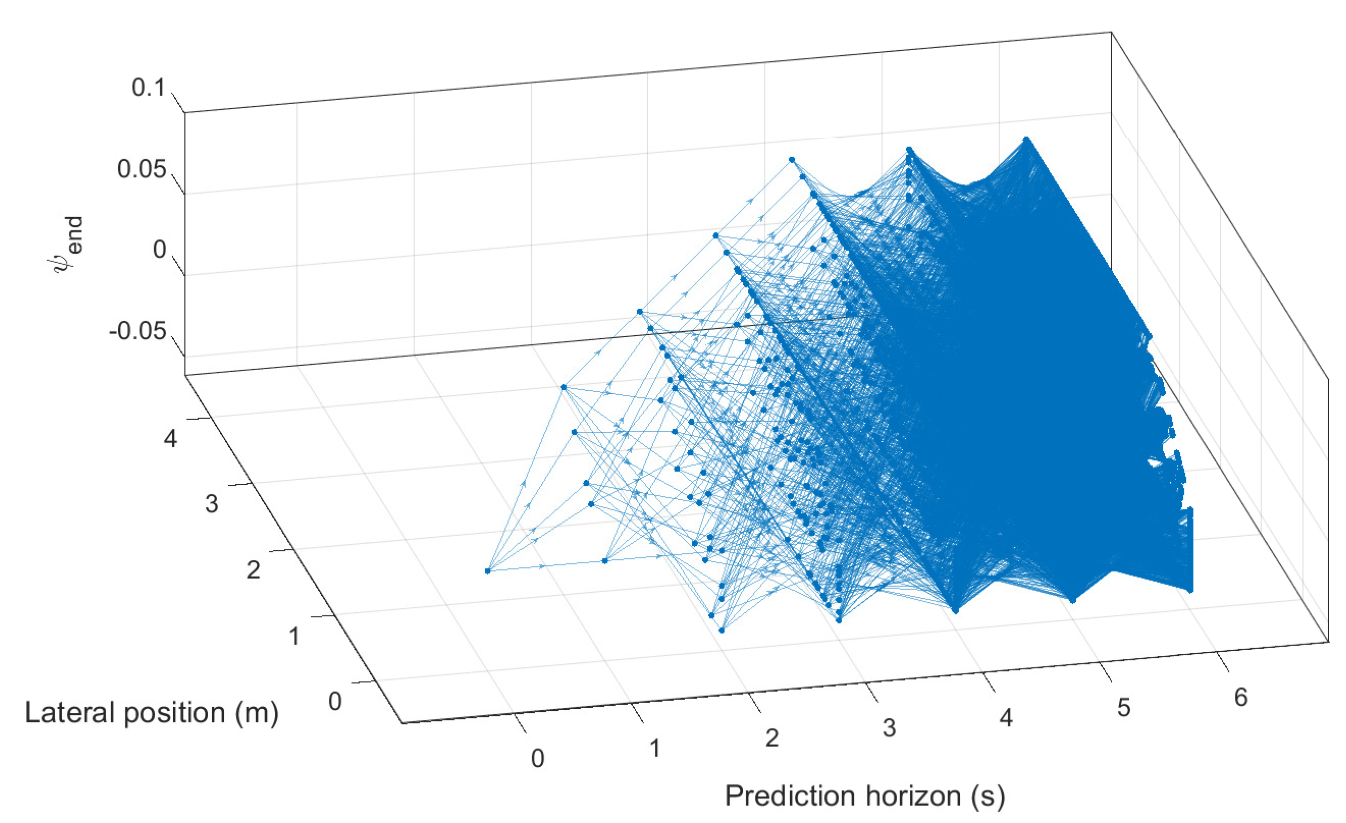
2.2. Computing the Lateral Positions of the Nodes

Firstly, the lateral positions of the nodes for the candidate vehicle trajectories are calculated. In the calculation, the limitation of the lateral acceleration is incorporated to avoid the skidding of the vehicle and uncomfortable trajectories. Since the lateral acceleration increases as the lateral position of the node increases, the inequality | c m a x , i | f ( x l , i , y l , i , ψ i n i t i a l , i ) for the limitation must be satisfied.Moreover, limitations on the lateral position y m i n y i y m a x is considered. Taking into consideration these limitations, the set of possible lateral positions can be computed ( Y ). In Figure 2 an example of the limitations can be seen. As it can be seen, the lateral position of n t h node cannot be selected to the value of y m a x since the lateral acceleration between the two nodes are higher than the previously defined maximum. However, the lateral position of the 1st node is limited with the road-specific constraint ( y m i n ) .
Secondly, the positions of the nodes in the given segment is determined. The main aspect during the computation of the lateral positions is to consider different types of maneuvers (e.g., overtaking another vehicle, avoiding an obstacle). In order to achieve this, the positions are computed using the lateral accelerations. The set of a c p , m a x , i can be computed ( A c p ). In the following step, the lateral positions are calculated as:
y i Y , a c p , i = m i n ( A c p ) + i ( m a x ( A c p ) m i n ( A c p ) ) N , c m a x , i = f ( x i , y i , ψ i n i t i a l , i ) i = 1 . . N ,
where N gives the number of nodes connected to the other node. Acceleration values are determined equidistantly. Using the computed lateral accelerations, the lateral positions of the given nodes can be calculated. The computation can be made along the whole prediction horizon. Using this method, the limitations on the lateral acceleration value can be guaranteed. Assuming that the vehicle moves into one direction in the given prediction horizon, this results in a directed graph, projected on the road:
G = ( V , E ¯ ) ,
where (V) gives the nodes, which are connected with the edges E ¯ . In Figure 3 an example is shown. In this case, the number of nodes connect to another is set to 5. The gray lines show the edges of the graph, and the blue curves are the feasible trajectories, which are computed by the predictive optimization method. The red curves are also the feasible trajectories, but these trajectories take place in the second layer of the graph (second step in the longitudinal direction).
In Figure 3 feasible trajectories can be found between the nodes. Since the initial yaw angle plays an important role during the trajectory planning, axis z represents the yaw angle of the vehicle at the end point of the designed trajectory. The lateral acceleration for each segment can be determined and this lateral acceleration series can be considered as an upper bound of the lateral acceleration of the whole trajectory.

2.3. Computing the Weights of the Edges

In this subsection, the weighting of the graph is presented. This weighting serves the purpose of keeping the lateral acceleration during the overtaking in a given value. During the calculation process of node positions of the candidate trajectories, the physical limits of the acceleration have already taken into account. The consideration of the lateral acceleration in weighting and the candidate trajectory computation is to guarantee the comfort and safety requirements at the same time. In Section 2 the calculation of the lateral accelerations are presented between two nodes. Using this information, and the following equations the weighting can be made.
W ( a l a t e r a l ) = κ 1 κ 2 a l a t e r a l a l a t , 1 i f a l a t e r a l < a l a t , 1 , θ 1 ( θ 2 a l a t e r a l ) 2 i f a l a t e r a l < a l a t , 2 , χ 1 + χ 2 a l a t e r a l otherwise ,
where ( κ , θ , χ ) are tuning parameters. Thus, when the maximum of lateral acceleration is smaller than a l a t , 1 , the weights must be increased in order to avoid maneuvers with lower time requirements. The preferred lateral acceleration value is chosen to a l a t , 2 and when the acceleration value exceeds the preferred one, the weights must be increased.

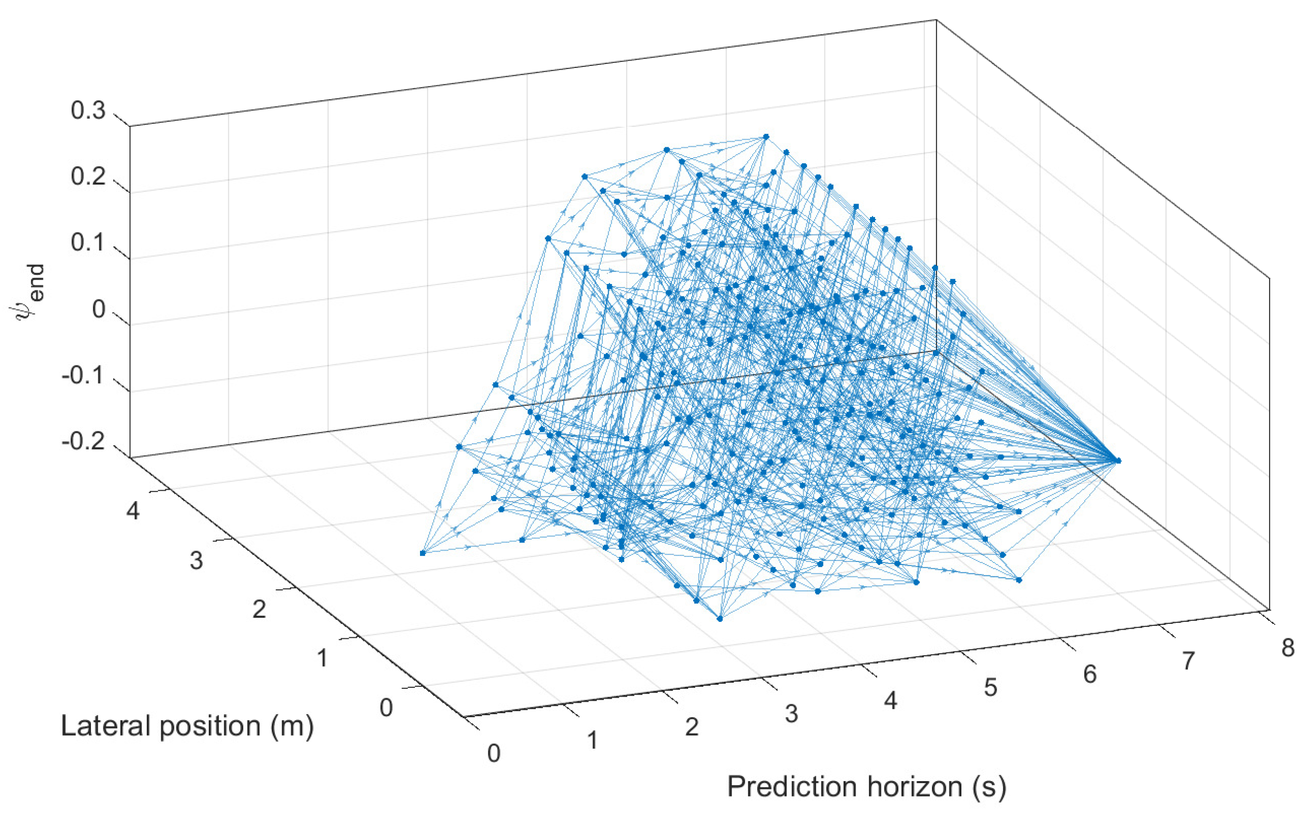
2.4. Reducing the Complexity of the Graph

In this subsection, the graph-based motion-planning algorithm is built up for the whole prediction horizon. The complexity of the problem increases exponentially according to the number of the layers since every node connects to n nodes. In order to reduce the complexity of the algorithm, the nodes which have nearly the same parameters are merged. This means, the nodes, which are closer to each other than a specified distance, are replaced with one node. To solve this, the k-medoids clustering algorithm [15] is used, which is a clustering algorithm and divides the nodes in a given layer into k subsets. This plays an important role in calculating probabilities of the collision, using the density functions. The k-medoids algorithm minimizes the distance between the nodes and the computed center of the given set ( η ). During the determination of the number of the clusters, which is the input of the clustering algorithm, the following inequality must be satisfied:
m a x ( η i v j ) y b , p 2 , v j V i V i V j = 1 n ,
where η i gives the center of the i t h set, and n is the number of the elements in the i t h subset and y b , p y b , where y b is a bound, which is defined in Equation (1). Moreover, for the presented new subsets (k), new bounds should be defined, which reflect on the probability of the collisions.
In the following example, a graph is built up, where the prediction horizon is set to T p = 6 s . One node connects to five other nodes. The number of layers was set to 6. This results in a large amount of possible points. Figure 4 shows the generated graph. As it is described in Section 2, the longitudinal positions of the nodes are set equidistantly. Since, the velocity of the ego vehicle ( v x ) is known, the longitudinal positions of the nodes computed to time t i = x i v x , i = 1 N . t i gives the value when the vehicle reaches the given node.
The total number of nodes, in this case, is 19,531. This graph cannot be used in the real-time implementation, because the processing of the graph requires high computational effort. In this case, the number of nodes is reduced from 19,531 to 240. The longitudinal position is changed to time which is necessary since the whole graph cannot be computed in real-time application. In this case, the calculated graph does not depend on velocity. Note that using the values of the curvatures and the velocity of the vehicle, the lateral acceleration can be computed. The result of the k-medoids algorithm is presented in Figure 5.

3. Motion Prediction of the Surrounding Vehicles

This section details the computation of the density functions which are used to predict the motion of the surrounding vehicles. This work is based on the widely used NGSIM dataset [16]. The data set consists of videos and other information on the participating vehicles such as their longitudinal and lateral positions, velocities and acceleration values using the sample time T s = 0.1 s . Furthermore, the length of the observed section is approximately 640 m and consists of five lanes. The whole video is recorded on a freeway in Los Angeles, California. Several researches deal with the evaluation of this dataset [17,18]. In the following subsections, the evaluation of the possible longitudinal and lateral motions of the vehicles is presented.

3.1. Lateral Motion of the Vehicle

The overtaking trajectories are collected from the NGSIM dataset. Due to the measurements, the collected vehicle trajectories can be noisy, and thus, feasible trajectories are fitted to the measured overtaking path. It can be said that one trajectory is feasible when the curvature of the trajectory is continuous and bounded. The basic idea behind this method is to build up the given trajectory using clothoid segments. Assuming clothoid segments, for the given overtaking trajectory, the curvature values can be computed. Since the velocities of the vehicles can be determined, the lateral accelerations can be computed. The value of lateral acceleration characterizes the overtaking trajectories, and the density functions are calculated based on these acceleration values. Assuming clothoid segments as a feasible trajectory, the coordinates of the smooth trajectory can be formulated as [19]:
x ( s ) = α π S s π , y ( s ) = α π C s π ,
where x ( s ) and y ( s ) the longitudinal and lateral direction of the clothoid segment, S ( x ) and C ( x ) denotes the Fresnel sine and cosine and a is the scaling factor. C ( L ) = 0 L c o s ( π t 2 2 ) d t , S ( L ) = 0 L s i n ( π t 2 2 ) d t . Using these formulas, the smooth trajectory can be built by clothoid segments, which guarantees the feasibility. Every trajectory is divided into four segments, where the sharpness parameter ( α ) characterizes the given segment. In Figure 6 an illustration on the overtaking trajectories and the computed smooth trajectories are depicted.
Using the fitted smooth trajectories, curvature can be determined as:
κ m = s l α ,
where s l is the length of the given segment. In the following step, the fitted, feasible trajectories are used to evaluate the overtaking maneuvers. The maximum curvature of the given segment can be computed using Equation (9). Since the velocity of the vehicles can be computed, the maximum value of lateral acceleration is calculated. In the next step, the prediction method of the lateral motion of the vehicle is presented. During the prediction method, the previously computed feasible trajectories and the longitudinal velocity of the vehicles which are provided by the NGSIM dataset, are used. As it is described below, the maximum lateral acceleration characterizes the overtaking scenarios. Density functions are fitted to the saved data, to solve the prediction process. During the determination of the density functions nearly 300 overtaking trajectories are selected from the whole NGSIM dataset, and at the same time, the velocity profile of the vehicles is saved of the given segment. Assuming the kinematic bicycle model, the lateral acceleration of the vehicle can be computed as it is described in Equation (2). Using the maximum values of the accelerations, the density function can be computed. The motion of the vehicles is predicted using the Gamma density function, which widely used in the field of predictions [20]. The advantage of this distribution is that it can be used for several motion models and it is easy to implement. The Gamma density function can be formed as:
f l a t ( x , α , β ) = β α x α 1 e β x Γ ( α ) ,
where x, α and β are non-negative. In Equation (10) Γ is the Gamma function which is formed as Γ ( α ) = 0 x α 1 e x d x , where α N . In Figure 7, the density and distribution functions are shown.
The probability can be computed between two lateral acceleration values as: P ( a l x a u ) = F ( a u ) F ( a l ) , where F is the distribution function. Using (8) the length of the possible trajectories can be determined since the velocity of the surrounding vehicles are measurable. The presented density and distribution functions are similar to previous ones, which can be found in the following research [21]. Xu et al. [22] determined the upper bound of the comfort level of the lateral acceleration to 3.6 m/s 2 . Considering the density functions, it can be said, that the probability of that cases when the lateral acceleration is below the comfort level is more than 90%. These results can be used to determine the optimal lateral acceleration value during a lane-change maneuver (see Section 2.3). The choice of this value is crucial, because if this value is chosen to be above a certain bound, the maneuver does not meet the comfort criteria. Otherwise, it takes too long to get to the other lane, which is unsatisfactory from the safety point of view.

3.2. Longitudinal Motion of the Vehicles

In the next step, the longitudinal motion of the vehicles is predicted. The computation of the density function is based on the NGSIM dataset. Firstly, a start point is selected randomly on the given road segment. The current longitudinal acceleration ( a c ) value is saved and assumed that the vehicle moves with it along the whole segment. The given horizon is predefined and the length of it is set to T = 8 s . The whole horizon is divided into 10 equidistant segments t [ t 1 , t 2 t n ] , n = 10 . The acceleration values at the previously defined time step t i are saved and compared to the acceleration value at the start point ( a c ) . The difference between them are recorded a d , i = a c a ( t i ) , i = 1 10 . During the determination of the density function associated with the longitudinal motions, the whole dataset is used unlikely to the lateral case.
The dataset is divided into disjoint sets ( A ) according to the initial acceleration values. a d , i A j , if a d , i { A l , j A u , j } and a d , i A j + 1 if k = 1 n , A l , k > A l , k + 1 and A u , k < A u , k + 1 . A l and A u denote the lower and upper bounds of the given set. To predict the possible longitudinal motion of the vehicles, Gaussian density functions are calculated to the previously computed sets. The Gaussian density function can be formulated as:
f k , i ( x ) = 1 σ 2 π e 1 2 ( x μ σ ) 2 k = 1 n ,
where k denotes the k t h prediction time step, and i gives the i t h set according to the initial acceleration as it is described below. Using these, the possible reachability areas can be determined, and also the probability of collisions during the motion-planning process. In Figure 8 the density functions are presented.
In Figure 8 the density functions are depicted where the bounds of accelerations are set to A l = 0.25 m / s 2 , A u = 0.25 m / s 2 . In the right side of the pictures the results are shown, in which the bounds are set to A l = 1 m / s 2 , A u = 1 m / s 2 . Note that at increased acceleration values, the uncertainty increases as well. The time step is set to t i = 0.8 s . The possible longitudinal and lateral movements are presented based on the NGSIM data. In the followings, these functions are used to predict the possible motions of the vehicles, and also help to compute the optimal value of the lateral acceleration, which is essential during the trajectory planning.

3.3. Prediction of the Vehicle Motion

The velocity of the controlled vehicle can be measured and assumed to be constant along the prediction horizon. The velocities and the distances measured from the controlled vehicle can be measured. The motion prediction of the surrounding vehicles is based on the NGSIM dataset, with which the density functions are computed. The lateral position of the vehicle is taken into account through the Gamma density function where the parameters of the density function are computed from the measurements Section 3.1. The longitudinal motion prediction is based on the Gaussian density functions, which is presented in Section 3.2. Motion-planning is made using the presented graph-based algorithm, in which weights are assigned to each node. The value of the weight depends on the maximum value of the lateral acceleration (see Section 2). An important step is to guarantee a collision-free trajectory during motion-planning. This can be made using the previously computed graph-based algorithm. Since the positions of the nodes are computed previously, based on the density functions and the measurements of the states of the surrounding vehicles, the probabilities can be computed. These values are added to the weighted graph. In order to guarantee a collision-free trajectory, the probabilities of the collision must be minimized along the reference trajectory.
The lateral motion of the vehicle can be predicted with the following equation:
P l a t ( y j ) = a m i n a m a x f l a t ( x , α , β ) d x · P w ( σ , μ ) ,
where f l a t is the Gamma density function and ( a m i n , a m a x ) is the set of the possible lateral accelerations. P w is responsible for taking into account the width of the vehicle, where y w is the width of the vehicle and variance is computed as σ = y w 4 . The μ gives the position of the center of the gravity of the vehicle. Moreover, the probabilities according to the longitudinal motion are also must be performed:
P ( x j , a d , i ) = 0 t i v x f j , i ( x ) d x ,
where v x gives the longitudinal velocity of the controlled vehicle. x j gives the longitudinal position of the graph node in the j t h time step, and a d , i is the current acceleration of the vehicle. Using Equation (12) and (13) the probability of collision can be computed to one node as:
P ( x j , y j , a d , i ) = P ( x j , a d , i ) · P l a t ( y j ) .
During the reduction of the graph, a bound ( y b , p ) has been defined in Equation (7). The maximum value of the probability is assigned to the given node:
P ( x m , y m ) = max ( P ( x j , y , a d , i ) ) y [ y m y b , p 2 , y m + y b , p 2 ] ,
where y b , p is the bound, which is used during the k-medoids algorithm, see Equation (7). Finally, to every node, the probabilities can be computed. The weights between to edges can be assigned as w : E ¯ R
w n = β ( P ( x m , y m ) ) + θ ( c · v x 2 ) ,
where ( x m , y m ) represents the coordinates of m t h node, which is connected with the n t h node and m > n . The curvature (c) can be easily computed from (4). Note that the collision free trajectory must be guaranteed, in order to achieve this, β and θ weighting functions can be used. This means the maximum value of the collision probability is assigned to the nodes.

4. Architecture of the Algorithm

4.1. Decision Making and Trajectory Generation

In the previous sections, the generation of the graph and the motion prediction of the surrounding vehicles are presented. The positions of the nodes are computed and using the approximating function, weights can be assigned to the edges. The surrounding vehicles must be taken into account. In order to achieve this, the probability of collision values is computed to the nodes. These values play an important role in the graph weighting. Using the weighted graph the main task is to compute a trajectory with the lowest sum of the values, which can be solved by a greedy algorithm. The output of the greedy algorithm is the nodes V 1 , V 2 V N , where N is the number of the layers. Since the graph is generated equidistantly in a longitudinal direction, the lateral positions are the main result of this algorithm. Using the computed reference positions, a neural-network calculates a feasible trajectory for the ego vehicle.

4.2. Checking the Probabilities of Collisions

Since the shortest path of the given graph can be computed using the greedy algorithm, the probability values for the reference trajectory is known. The reference trajectory is defined by the nodes V i , i = 1 n . The greedy algorithm computes the edges with the lowest sum of weights. There can be cases, in which even the lowest sum of the weights does not guarantee collision-free trajectory, e.g., a weight of one node is high, the other ones are low, this results in a low sum of the weights. In order to guarantee the collision-free trajectory, the probability values P ( v i ) must be checked. After defining the maximum value of the probability ( ϵ ), the following inequality must be satisfied:
P ( v i ) ϵ , i .
There may be cases when these bounds are violated. Then the longitudinal position of the ego vehicle must satisfies the following bounds: x e g o , i < x d , i where x d , i is the modified longitudinal coordinate of the i-th node. Since the density functions are known, (see Section 3.2), x d , i can be computed ϵ = 0 x d , i f ( x ) d x . Using these longitudinal coordinates the states of the vehicle can be bounded in the given time steps, using e.g., a model predictive control. Further information can be found in [23]. Since the curvatures can be computed from the trajectory, the longitudinal motion of the vehicle can be designed taking into account the maximum value of the combined acceleration.

4.3. Structure of the Algorithm

Finally, in Figure 9, the structure of the algorithm is introduced.
In Figure 9 the scheme of the algorithm is presented. The blue-colored rectangles represent that parts of the algorithm, which are responsible for the process of the a priori data. The red parts show the operation of the algorithm. In Section 3 the NGSIM dataset is detailed, and in Section 3.1 and Section 3.2 the computation of the density functions, which are used in longitudinal and lateral motion predictions, are presented. After computing the trajectory, the probabilities of the collisions are checked in Section 4. If the values of the probabilities are higher than a previously defined maximum, the longitudinal velocity of the vehicle must be varied. The rest of the layer is related to the computation of the feasible trajectories. The generation of the graph, using the calculated maximum value of the lateral acceleration is detailed in Section 2. The calculation of the feasible trajectories which are used during the neural network training process is described in Appendix A. The training of the neural network is achieved through a previously-generated dataset, and the results of the trained neural network are validated using the test dataset. The results of the neural network showed appropriate results. However, safety performances can be guaranteed, using a robust control framework [10]. Finally, the longitudinal motion of the vehicle is taken into account.

5. Simulation Example

In this subsection, a traffic situation is solved using the graph-based motion-planning algorithm. In Figure 10, the points are presented, where the algorithm is evaluated. During the graph generation the value of y p , b is set to 0.1 m .
First, the motion of the vehicle is predicted, and then the probability values and the weights are computed. The shortest path of the proposed graph can be found using Dijkstra’s algorithm, which is a greedy algorithm. Using the reference vector, the neural network trajectory planning algorithm is evaluated, and finally, the trajectory is tracked by a local controller, where one nonlinear bicycle model is used. The velocity of the ego vehicles are set to v x = 20 m / s , v other = 15 m / s The distance between them is d = 16 m , and the acceleration value on the first time step is a o t h e r = 1 m / s 2 . The lateral position of the vehicle in the front is y o t h e r = 0 m . Finally, the width of the vehicle is set to w o t h e r = 2.2 m . In Figure 11 the results for the 1st point are presented. It can be seen, that the vehicle can track the reference trajectory, which is computed by the neural network.
It can be said, that the result of the simulations shows, that the algorithm decided to overtake, and the smooth trajectory is planned by the neural network. The local controller of the ego vehicle was able to track the reference trajectory, and the lateral accelerations during the simulation were nearly at the comfort level which is 1.6 m / s 2 . During the second part of the simulations, only the planned trajectories are presented. Since the goal of this paper is to introduce a motion-planning algorithm, in these cases, the planned trajectory is not tracked by the controlled vehicle. In Figure 12 and Figure 13 the planned trajectories, and the results of the graph-based algorithm are presented.
As it can be seen, the algorithm makes the correct decision in different cases, and using the results, the neural network-based algorithm planned the feasible trajectory. In Figure 12 the result of the algorithm can be seen for the second and third cases. The ego vehicle must get to the another lane to avoid the collision with the other vehicle. Finally, in Figure 13, the vehicle gets back to the original lane after overtaking the vehicle, which was in front of the controlled vehicle. In Table 1, the differences between the planned trajectory, and the reference vector are showed.
Table 1 shows the maximum value of the differences between the reference vector, provided by the graph-based algorithm, and the computed feasible trajectory. The maximum value of the error is 0.435 m. It can be said that the maximum values of the errors are smaller than the maximum value during the generation of the trajectories (see: Appendix A.3). It can be said, that the graph-based algorithm can compute the collision-free trajectory. Using a machine learning-based approach, the feasible trajectory is planned using the results of the graph-based algorithm.

6. Conclusions

In this paper, a graph-based motion-planning algorithm is presented. During the generation of the graph, several constraints are taken into account in order to guarantee the safety and comfort requirements at the same time. The motion prediction of the surrounding vehicles is made by the density functions which are generated using NGSIM data. The weights of the directed graph are calculated from the probabilities of collisions and the maximum value of lateral accelerations. The output of the graph-based algorithm is the reference points, with which the neural network-based algorithm computes the feasible trajectory. The proposed algorithm is validated through one comprehensive simulation. The results show that the algorithm is able to determine the collision-free trajectory, and the trajectory satisfies the bounds.

Author Contributions

Conceptualization, algorithms, software, T.H.; methodology, T.H. and B.N.; supervision, P.G. All authors have read and agreed to the published version of the manuscript.

Funding

This research received no external funding.

Acknowledgments

The paper was partially funded by the National Research, Development and Innovation Office (NKFIH) under OTKA Grant Agreement No. K 135512 and under the National Laboratory for Autonomous Systems. The work of Balázs Németh was partially supported by the János Bolyai Research Scholarship of the Hungarian Academy of Sciences and the ÚNKP-20-5 New National Excellence Program of the Ministry for Innovation and Technology from the source of the National Research, Development and Innovation Fund. The work of Tamás Hegedűs has been supported by the ÚNKP-20-3 New National Excellence Program of the Ministry for Innovation and Technology from the source of the National Research, Development and Innovation Fund.

Conflicts of Interest

The authors declare no conflict of interest.

Appendix A. Trajectory Planning

Appendix A.1. The Lateral and Longitudinal Model of the Vehicle

During the trajectory planning for the controlled vehicle the well-known two-wheeled lateral vehicle model is used, which is introduced by Rajamani [24], and includes the following equations:
m v x ( ψ ˙ + β ˙ ) = C 1 α 1 + C 2 α 2 ,
I z ψ ¨ = C 1 α 1 l 1 C 2 α 2 l 2 ,
v ˙ y = v x ( ψ ˙ + β ˙ ) ,
where I z is the yaw inertia, m is the mass of the vehicle C 1 , C 2 are the cornering stiffness of the front and rear tires. Furthermore, l 1 , l 2 is the distances of the front and rear axes measured from the center of the gravity of the vehicle. The side-slip angles can be computed using equation: α 1 = δ β ψ ˙ l 1 / v x and α 2 = β + ψ ˙ l 2 / v x . Using Equation (Appendix A.1), the state space representation of the system can be written in the following form:
x ˙ = A x + B u ,
y = C T x + D u ,
where u is the steering angle ( δ ). The proposed dynamic model is used during the trajectory planning.
Moreover, during the longitudinal motion prediction of the surrounding vehicles, a constant acceleration is assumed. Using this assumption the following equation gives the position to the ( k + 1 ) t h time step:
s ( k + 1 ) = s ( k ) + v ( k ) t + 1 2 a ( k ) t 2 ,
where a ( k ) gives the longitudinal acceleration and v ( k ) is the velocity in the k t h time step.

Appendix A.2. Predictive Optimization Method

A predictive control-based trajectory planning is presented in this section, and then the Neural Network-based method is used to make the trajectory planning faster since the computation of the quadratic optimization function is time-consuming. The results of the model predictive optimization approach are used to compute the weights of the edges which are used in the motion-planning layer. The basis of the discretized state space representation is the dynamic bicycle model (see: Equation (Appendix A.1)), which can be written in the following form:
x ( k + 1 ) = ϕ x ( k ) + Γ u ( k ) ,
where ϕ = e A T s and Γ = k T s ( k + 1 ) T s e A ( ( K + 1 ) T s τ ) B d τ . The states of the discrete state space representation are: x = y v y ψ ˙ ψ δ T . In order to minimize the lateral acceleration, the output of the model is the lateral position and lateral acceleration of the controlled vehicle. Using Equation (A6) the output matrix can be formed as: C = 1 0 0 0 0 0 0 0 0 v x 2 l 1 + l 2 .
In this case, the lateral acceleration of the vehicle can be approximated as a l a t = v x 2 R . Using the kinematic bicycle model, the radius of the given trajectory can be computed as:
R = l 1 + l 2 t a n ( δ )
Assuming small angles: t a n ( δ ) δ . The lateral acceleration of the vehicle can be approximated by the following equation:
a l a t = v x 2 δ l 1 + l 2 .
The error, which is measured from the reference vector, can be defined as Németh et al. [9]:
e y = y ( U ) R ,
where R is the reference lateral position of the vehicle. The control signal is computed through the minimization process. The minimization function can be written as
J ( U , x ( k ) ) = 1 2 i = k n + k e y ( U ) T ξ e y ( U ) + U T λ U ,
where U = u ( k ) u ( k + n ) T . Moreover, ξ and λ are weighting matrices. This leads to a quadratic optimization problem, which can be formulated as
min u ( k + 1 ) , u ( k + 2 ) u ( k + n ) J ( U , x ( k ) ) s . t . H i n U < b l l u i l u ,
where H i n is responsible for the limitation of the states. Which can be computed from the dynamics of the controlled vehicle. During the trajectory planning, several constraints must be defined to the states in order to guarantee the safety and comfort requirements. Control input of the system also must be limited within ( l l , l u ) , taking into account the limitations of a real system.
During the trajectory planning several limitations must be taken into account in order to guarantee the safety and comfort requirements. The optimization problem is solved with the following limitations:
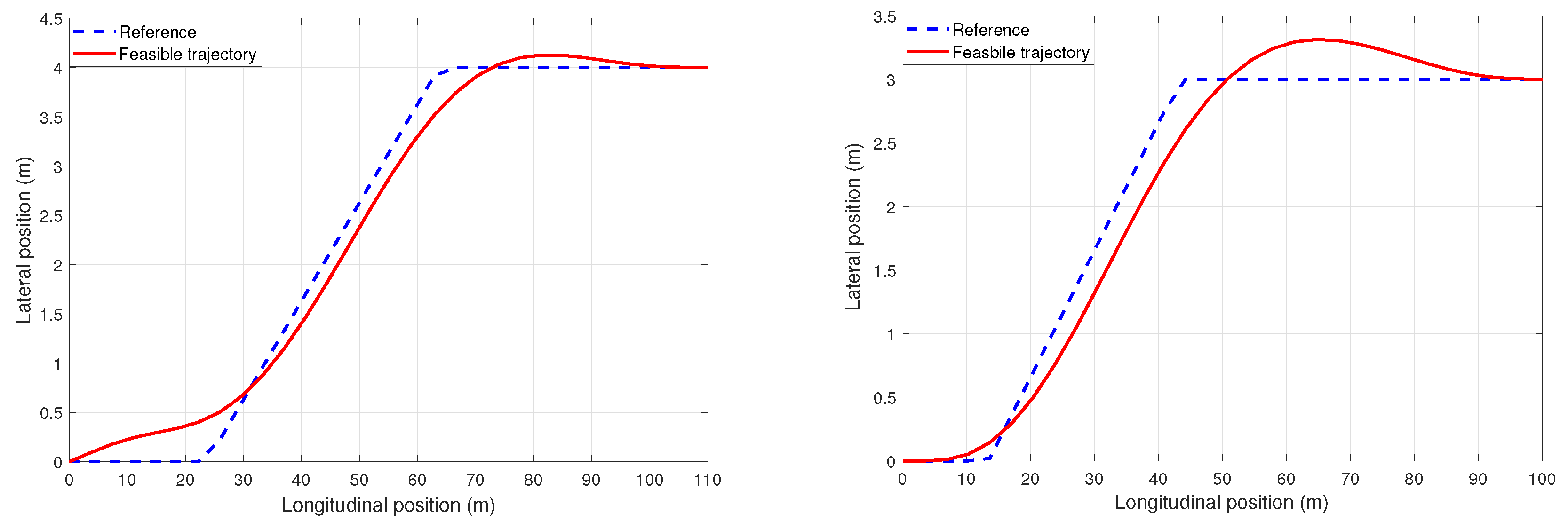
  • Lateral position. It is necessary to limit the lateral error measured from the reference trajectory in order to avoid dangerous motion of the vehicle. Moreover, it is important to guarantee that the reference lateral position is reached by the planned trajectory at the end point. During the computation, the maximum deviation measured from the reference trajectory is set to | e m a x | = 0.5 m .
  • Yaw angle. Another important point of the trajectory planning is the yaw angle of the vehicle. The feasible trajectory must ensure that the yaw angle of the vehicle is the same as the yaw angle of the reference trajectory.
  • Steering angle. The steering angle and its rate must be also bounded. Δ δ m i n Δ δ Δ δ m a x and δ m i n δ δ m a x , where the bounds can be calculated from the limits of the actuator. Moreover the limitations help to guarantee comfort and safety requirements.
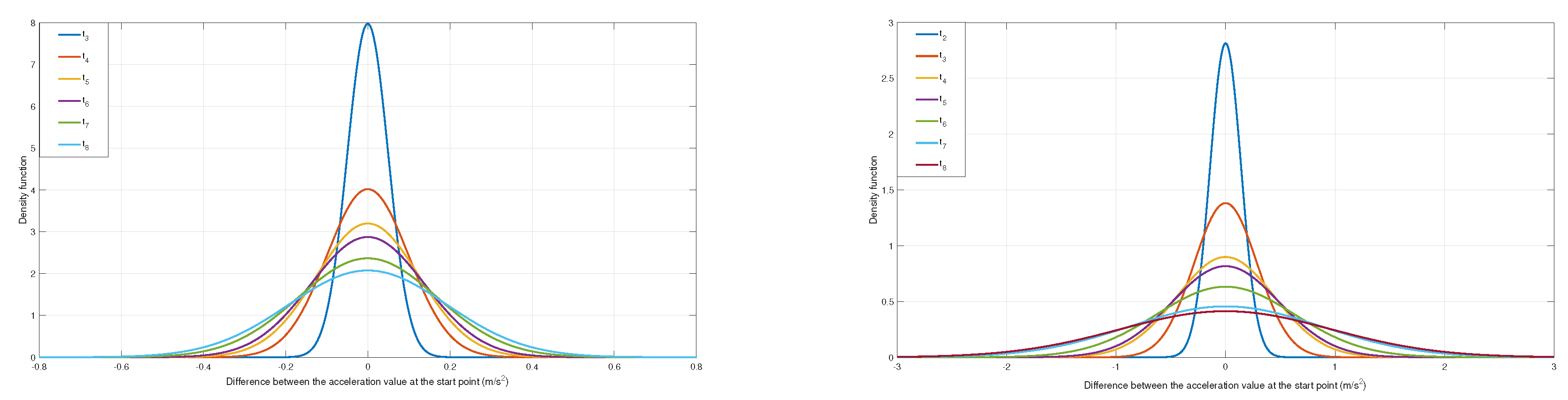
  • Lateral acceleration. During the trajectory planning, the lateral acceleration is minimized. Using the computed data (see Section 3.1), the bounds are set to a l a t , b | a l a t | . Where a l a t , b is set to 4 m / s 2 . More than 95% of the computed maximum accelerations are above this value (Figure 7).
An example for the trajectory planning is shown in Figure A1.
Figure A1. Computed trajectories.
Applsci 10 07716 g0a1

Appendix A.3. Neural Network Based Trajectory Planning

Since the optimization process can be time-consuming, during the implementation the trajectory planning is performed through a machine learning-based approach. In order to train the machine learning-based model, a lot of data needed. Therefore, several trajectories have been planned using the proposed algorithm with different parameter sets. There are several machine learning algorithms which can deal with the trajectory planning problem [25]. However, in general, the most flexible solution is provided by the neural networks, since they are capable to solve complex and nonlinear problems. Therefore, in this paper a neural network-based solution is applied to solve this problem [11]. The trained neural network consists of one input, one output, and three hidden layers. Since, the number of neurons can be chosen freely, to determine the optimal number of them, the so-called k-cross validation technique is used. The mentioned method divides the training data into subsets. The first subset is used to train the network, and at the same time, another randomly created subsets are used to validate it. The number of neurons in the hidden layer is chosen to be 18-10-16. As it is described, the activation functions have to be chosen. In this paper, the rectified linear unit (ReLU) and the log-sigmoid functions are used in the network, since these functions can be used to solve nonlinear problems. The training process is based on the widely used Levenberg–Marquardt algorithm [26]. References

References

  1. Ziebinski, A.; Cupek, R.; Erdogan, H.; Waechter, S. A Survey of ADAS Technologies for the Future Perspective of Sensor Fusion. In Proceedings of the Computational Collective Intelligence, Halkidiki, Greece, 28–30 September 2016. [Google Scholar]
  2. Hasenjager, M.; Heckmann, M.; Wersing, H. A Survey of Personalization for Advanced Driver Assistance Systems. IEEE Trans. Intell. Veh. 2019, 5, 335–344. [Google Scholar] [CrossRef]
  3. Nemeth, B.; Gaspar, P.; Hegedus, T. Optimal Control of Overtaking Maneuver for Intelligent Vehicles. J. Adv. Transp. 2018, 2018. [Google Scholar] [CrossRef]
  4. Fu, X.; Jiang, Y.; Lu, G.; Wang, J.; Huang, D.; Yao, D. Probabilistic Trajectory Prediction in Intelligent Driving. IFAC Proc. Vol. 2014, 47, 2664–2672. [Google Scholar] [CrossRef]
  5. Hegedus, T.; Nemeth, B.; Gaspar, P. Graph-based Multi-Vehicle Overtaking Strategy for Autonomous Vehicles. In Proceedings of the 9th IFAC Symposium on Advances in Automotive Control (AAC), Orléans, France, 21–22 June 2019; pp. 372–377. [Google Scholar]
  6. Yoon, S.; Kum, D. The Multilayer Perceptron Approach to Lateral Motion Prediction of Surrounding Vehicles for Autonomous Vehicles. In Proceedings of the IEEE Intelligent Vehicles Symposium (IV), Gotenburg, Sweden, 19–22 June 2016; pp. 1307–1312. [Google Scholar]
  7. Xu, W.; Pan, J.; Wei, J.; Dolan, J.M. Motion Planning under Uncertainty for On-Road Autonomous Driving. In Proceedings of the 2014 IEEE International Conference on Robotics and Automation (ICRA), Hong Kong, China, 31 May–5 June 2014; pp. 2507–2512. [Google Scholar]
  8. Tsitsiklis, J.N. Efficient algorithms for globally optimal trajectories. IEEE Trans. Autom. Control. 1995, 40, 1528–1538. [Google Scholar] [CrossRef]
  9. Nemeth, B.; Hegedus, T.; Gáspár, P. Model Predictive Control Design for Overtaking Maneuvers for Multi-Vehicle Scenarios. In Proceedings of the 2019 18th European Control Conference (ECC), Naples, Italy, 25–28 June 2019; pp. 744–749. [Google Scholar]
  10. Nemeth, B.; Hegedus, T.; Gaspar, P. Performance Guarantees on Machine-Learning-based Overtaking Strategies for Autonomous Vehicles. In Proceedings of the 2020 European Control Conference (ECC), Saint-Petersburg, Russia, 12–15 May 2020; pp. 136–141. [Google Scholar]
  11. Hegedus, T.; Nemeth, B.; Gaspar, P. Multi-objective trajectory design for overtaking maneuvers of automated vehicles. In Proceedings of the IFAC World Congress 2020, Berlin, Germany, 12–17 July 2020. [Google Scholar]
  12. Ji, X.; He, X.; Lv, C.; Liu, Y.; Wu, J. Adaptive-neural-network-based robust lateral motion control for autonomous vehicle at driving limits. Control. Eng. Pract. 2018, 76, 41–53. [Google Scholar] [CrossRef]
  13. Berntorp, K. Path Planning and Integrated Collision Avoidance for Autonomous Vehicles. In Proceedings of the 2017 American Control Conference, Washington, DC, USA, 24–26 May 2017; pp. 4023–4028. [Google Scholar]
  14. Berntorp, K.; Magnusson, F. Hierarchical Predictive Control for Ground-Vehicle Maneuvering. In Proceedings of the 2015 American Control Conference, Chicago, IL, USA, 1–3 July 2015; pp. 2771–2776. [Google Scholar]
  15. Cao, D.; Yang, B. An improved k-medoids clustering algorithm. In Proceedings of the 2nd International Conference on Computer and Automation Engineering (ICCAE), Singapore, 26–28 February 2010; pp. 132–135. [Google Scholar]
  16. U.S. Department of Transportation. NGSIM—Next Generation Simulation. 2008. Available online: https://ops.fhwa.dot.gov/trafficanalysistools/ngsim.htm (accessed on 15 July 2020).
  17. Coifman, B.; Li, L. A critical evaluation of the Next Generation Simulation (NGSIM) vehicle trajectory dataset. Transp. Res. Part Methodol. 2017, 105, 362–377. [Google Scholar] [CrossRef]
  18. Punzo, V.; Borzacchiello, M.T.; Ciuffo, B. On the assessment of vehicle trajectory data accuracy and application to the Next Generation SIMulation (NGSIM) program data. Transp. Res. Part Emerg. Technol. 2011, 19, 1243–1262. [Google Scholar] [CrossRef]
  19. Gray, A. Modern Differential Geometry of Curves and Surfaces; CRC Press: Boca Raton, FL, USA, 1993. [Google Scholar]
  20. Mahapatra, G.; Maurya, A.K. Dynamic parameters of vehicles under heterogeneous traffic stream with non-lane discipline: An experimental study. J. Traffic Transp. Eng. 2018, 5, 386–405. [Google Scholar] [CrossRef]
  21. Asaithambi, G.; Shravani, G. Overtaking behaviour of vehicles on undivided roads in non-lane based mixed traffic conditions. J. Traffic Transp. Eng. 2017, 4, 252–261. [Google Scholar] [CrossRef]
  22. Xu, J.; Yang, K.; Shao, Y.; Lu, G. An Experimental Study on Lateral Acceleration of Cars in Different Environments in Sichuan, Southwest China. Discret. Dyn. Nat. Soc. 2015, 6, 1–16. [Google Scholar] [CrossRef] [Green Version]
  23. Matute-Peaspan, J.A.; Marcano, M.; Zubizarreta, A.; Perez, J. Longitudinal Model Predictive Control with comfortable speed planner. In Proceedings of the 2018 IEEE International Conference on Autonomous Robot Systems and Competitions (ICARSC), Torres Vedras, Portugal, 25–27 April 2018; pp. 136–141. [Google Scholar]
  24. Rajamani, R. Vehicle Dynamics and Control; Springer: New York, NY, USA, 2005. [Google Scholar]
  25. Chen, J.; Zhao, P.; Liang, H.; Mei, T. Motion Planning for Autonomous Vehicle Based on Radial Basis Function Neural Network in Unstructured Environment. Sensors 2014, 14, 17548–17566. [Google Scholar] [CrossRef] [PubMed] [Green Version]
  26. Demut, H.; Hagan, M.; Beale, M. Neural Network Design; PWS Publishing Co: Boston, MA, USA, 1997. [Google Scholar]
Figure 1. Trajectories between three points.
Applsci 10 07716 g001
Figure 2. Limitations during the graph generation.
Applsci 10 07716 g002
Figure 3. An example for the graph.
Applsci 10 07716 g003
Figure 4. Graph used during the motion-planning process.
Applsci 10 07716 g004
Figure 5. Recalculated graph for the motion-planning algorithm.
Applsci 10 07716 g005
Figure 6. Comparing the raw data to the smooth trajectories.
Applsci 10 07716 g006
Figure 7. Density and distribution function of the lateral accelerations.
Applsci 10 07716 g007
Figure 8. Density functions of the longitudinal motion.
Applsci 10 07716 g008
Figure 9. Structure of the algorithm.
Applsci 10 07716 g009
Figure 10. The traffic scenario.
Applsci 10 07716 g010
Figure 11. Results of the simulation.
Applsci 10 07716 g011
Figure 12. Result of the algorithm in cases 2 and 3.
Applsci 10 07716 g012
Figure 13. Result of the algorithm in cases 4 and 5.
Applsci 10 07716 g013
Table 1. The maximum values of the errors.
Case12345
Error (from NN) (m)0.3120.2580.1610.4350.419
Sample Availability: Samples of the compounds are available from the authors.
Publisher’s Note: MDPI stays neutral with regard to jurisdictional claims in published maps and institutional affiliations.

