1. Introduction
The purpose of optimization is to determine the best solution among the available solutions for an optimization problem according to the constraints of problem [
1]. Each optimization problem is designed with three parts: constraints, objective functions, and decision variables [
2]. There are many optimization problems in different sciences that should be optimized using the appropriate method. Stochastic search-based optimization algorithms have always been of interest to researchers in solving optimization problems [
3]. Optimization algorithms are able to provide a quasi-optimal solution based on random scan of the search space instead of a full scan. The quasi-optimal solution is not the best solution, but it is close to the global optimal solution of the problem [
1]. In this regard, optimization algorithms have been applied by scientists in various fields such as energy [
4,
5,
6], protection [
7], electrical engineering [
8,
9,
10,
11,
12,
13], topology optimization [
14] and energy carriers [
15,
16,
17] to achieve the quasi-optimal solution.
Table 1 shows the optimization algorithms grouped according to the main design idea.
Each optimization problem has a definite solution called a global solution. Optimization algorithms provide a solution based on random search of the search space, which is not necessarily a universal solution, but because it is close to the optimal solution, it is an acceptable solution. The solution that is provided by optimization algorithms is called quasi-optimal solution. Therefore, an optimization algorithm that offers a better quasi-optimal solution than another algorithm is a better optimizer algorithm. In this regard, many optimization algorithms have been proposed by researchers to solve optimization problems and achieve to the better quasi-optimal solution.
Although optimization algorithms have been successful in solving many optimization problems, improving the equations of optimization algorithms and adding modification phases to optimization algorithms can lead to better quasi-optimal solutions. In fact, the purpose of improving an optimization algorithm is to increase the ability of that algorithm to more accurately scan the problem search space and thus provide a more appropriate quasi-optimal solution and closer to the global optimal solution.
In this paper, a new modification method called Dehghani method (DM) is proposed to improve the performance of optimization algorithms. DM is designed based on the use of the algorithm population members information. In the proposed DM, the information of each population member can improve the situation of the new generation. The main idea of DM is to amplify the best population member of an optimization algorithm using population member information. The proposed method is fully described in the next section.
The continuation of the present article is organized in such a way that in
Section 2, the DM is fully explained and modeled. Following this,
Section 3 explains how to implement the proposed method on several algorithms. The simulation of the proposed method for solving optimization problems is presented in
Section 4. Finally, conclusions and several suggestions for future studies are presented in
Section 5.
2. Dehghani Method (DM)
In this section, first DM is explained and then its mathematical modeling is presented. DM shows that all population members of the optimization algorithm, even the worst one, can contribute to the development of the population of algorithm.
Each population-based optimization algorithm has a matrix called the population matrix, which each row of this matrix represents a population member. Each member of the population is actually a vector which represents the values of the problem variables. Given that each member of the population is a random vector in the problem search space, it is a suggested solution (SS) to the problem. After the formation of the population matrix, the values proposed by each population member for the problem variables are evaluated in the objective function (OF). The population matrix and values of the objective functions are defined in Equation (1).
where,
is the suggested solutions matrix,
is the population matrix,
is the
i’th suggested solution,
is the
i’th population member,
is the value of
d’th variables of optimization problem suggested by
i’th population member,
is the number of population members or suggested solutions,
is the number of variables, and
is the value of objective function for the
i’th suggested solution.
Different values for the objective function are obtained based on the values proposed for the variables by the population members. The member that offers the best-suggested solution (BSS) to the optimization problem plays an important role in improving the algorithm population. The row number of this member in the population matrix is determined using Equation (2).
where,
is the row number of the member with BSS. The BSS and it’s
OF are specified by Equations (3) and (4).
where,
is the BSS or best population member and
is the value of
OF for BSS.
As mentioned, the best member of the population plays an important role in improving the population of the algorithm and thus the performance of the optimization algorithm. Optimization algorithms update the status of its population members according to its own process to achieve a quasi-optimal solution. Accordingly, with the improvement of the best member of the population, is expected that the population be updated more effectively and the performance of the algorithm in solving the optimization problem is improved.
DM is designed with the idea of modifying the best population member with the aim of improving the performance of an optimization algorithm.
In DM, just as the best member is influential in updating the population members, the population members even the worst member can influence to modification the best member. The measurement criterion for suggested solutions is the value of the objective function. However, a suggested solution that is not the best solution may provide appropriate values for some problem variables. The proposed DM modifies the best member considering this issue and using the values suggested by other of the population members. This concept is mathematically simulated in Equations (5) and (6).
where,
is the modified best member by DM,
is the modified best member based on the suggested value for
d’th variable by
i’th SS,
is the new status for best member based on DM, and
is the objective function value for modified best member by DM.
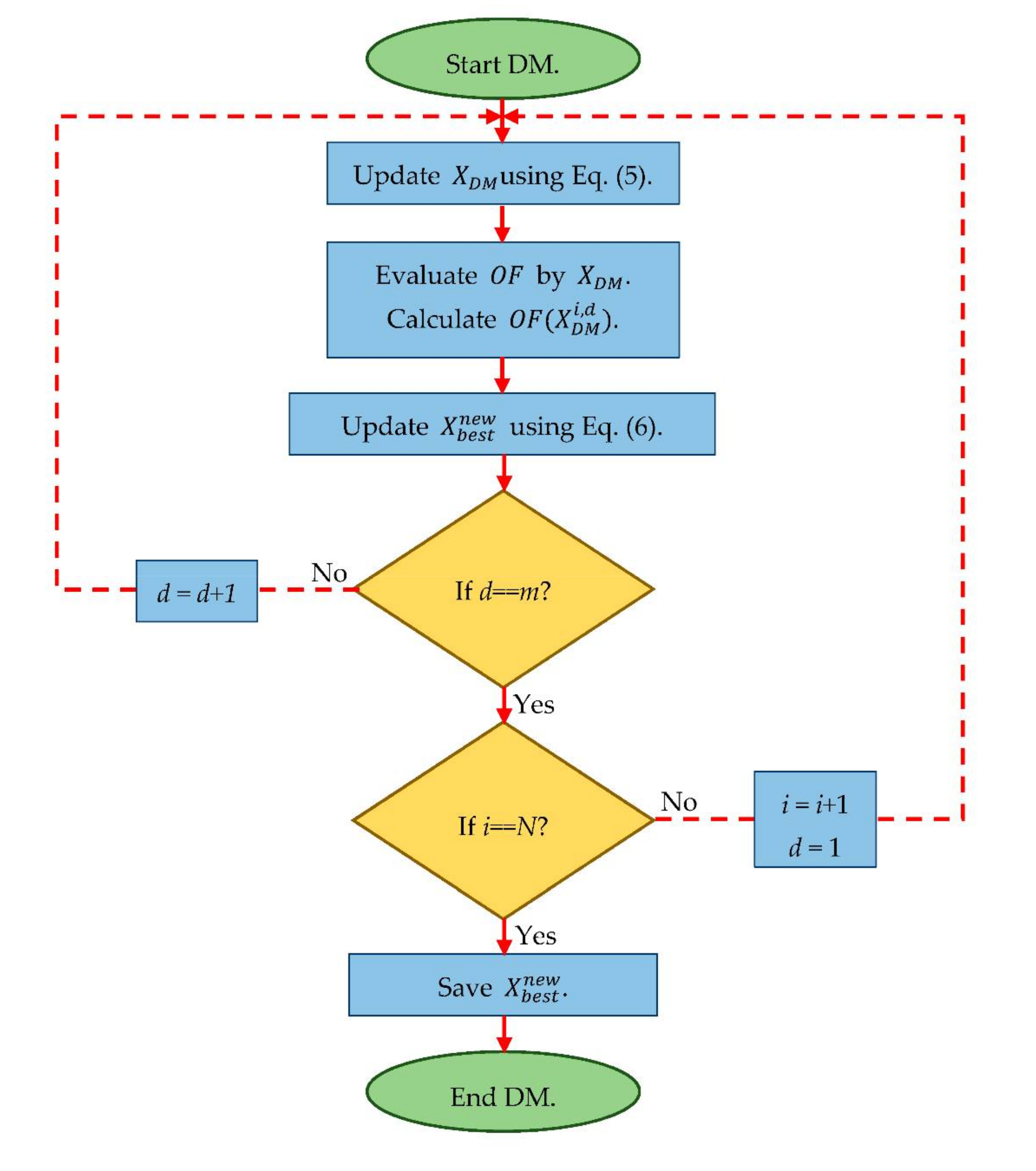
The pseudo code of DM is presented in Algorithm 1. In addition, the different stages of the proposed method with the aim of improving the best member are shown as a flowchart in
Figure 1.
| Algorithm 1. Pseudo code of DM |
| 1. | For i = 1:Npopulaion | Npopulaion: number of population members. |
| 2. | For d = 1:m | m: number of variables. |
| 3. | Update using Equation (5). |
| 4. | Calculate . |
| 5. | Update using Equation (6): |
| 6. | If |
| 7. | = |
| 8. | End if |
| 9. | End for d |
| 10. | End: for i |
3. DM Implantation on Optimization Algorithms
This section describes how to implement the proposed DM on optimization algorithms. The proposed DM is applicable to modify population-based optimization algorithms. Although the idea of designing optimization algorithms is different, the procedure is the same. These algorithms provide a quasi-optimal solution starting from a random initial population and following a process based on repetition and population updates in each iteration.
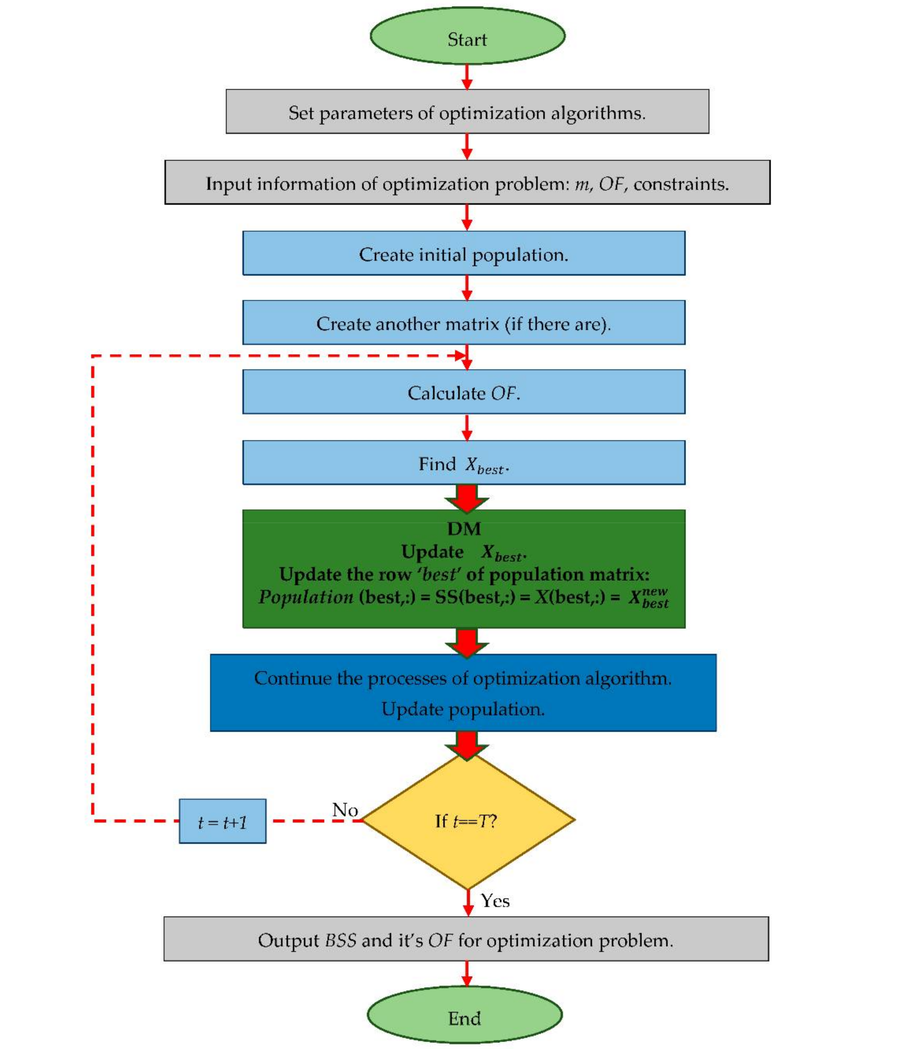
The pseudo code of implantation of the DM for modifying optimization algorithms is presented in Algorithm 2. The steps of the modified version of the optimization algorithms using DM are shown in
Figure 2.
| Algorithm 2. Pseudo code of implantation of the DM for modifying optimization algorithms |
| Start. |
| 1. | Set parameters. |
| 2. | Input: m, OF, constraints. |
| 3 | Create initial population. |
| 4. | Create another matrix (if there are). |
| 5. | For t = 1: iterationmax | iterationmax: maximum number of iterations. |
| 6. | Calculate OF. |
| 7. | Find . |
| 8. | DM toolbox: |
| 9. | Update based on DM. |
| 10. | Continue the processes of optimization algorithm. |
| 11. | Update population. |
| 12. | End for t |
| 13. | Output: BSS. |
| End. |
4. Simulation and Discussion
In this section, the performance of the proposed DM in improving optimization algorithms is evaluated. Thus, the present work and the optimization algorithms described in [
18,
29,
32,
50,
53] are developed using the same computational platform: Matlab R2014a (8.3.0.532) version in the environment of Microsoft Windows 10 with 64 bits on Core i-7 processor with 2.40 GHz and 6 GB memory. To generate and report the results, for each objective function, optimization algorithms utilize 20 independent runs where each run employs 1000 times of iterations.
4.1. Algorithms Used for Comparisons and Benchmark Test Functions
To evaluate the performance of the proposed DM, the following methodology is applied:
- (1)
Find in the literature five well-known optimization algorithms, such as: genetic algorithm (GA) [
50], particle swarm optimization (PSO) [
18], gravitational search algorithm (GSA) [
53], teaching learning based optimization (TLBO) [
29] and grey wolf optimizer (GWO) [
32].
- (2)
Modify the optimization algorithms implementing the proposed DM.
- (3)
Define the set of twenty-three objective functions and divide it into three main categories: unimodal [
53,
54], multimodal [
31,
54], and fixed-dimension multimodal [
54] functions (see
Appendix A).
- (4)
Implement the present work and the optimization algorithms in the same computational platform.
- (5)
Compare the performance of the modified and the original optimization algorithms using the following metrics: the average and the standard deviation of the best obtained optimal solution till the last iteration is computed.
4.2. Results
Optimization algorithms in the original version and the modified version, using the proposed DM, are implemented on the objective functions. The simulation results are presented from
Table 2,
Table 3,
Table 4,
Table 5 and
Table 6 for three different categories: unimodal, multimodal, and fixed-dimension multimodal functions. The first category consists of seven objective functions, F
1 to F
7, the second category consists of six objective functions, F
8 to F
13, and the third category consists of ten objective functions, F
14 to F
23.
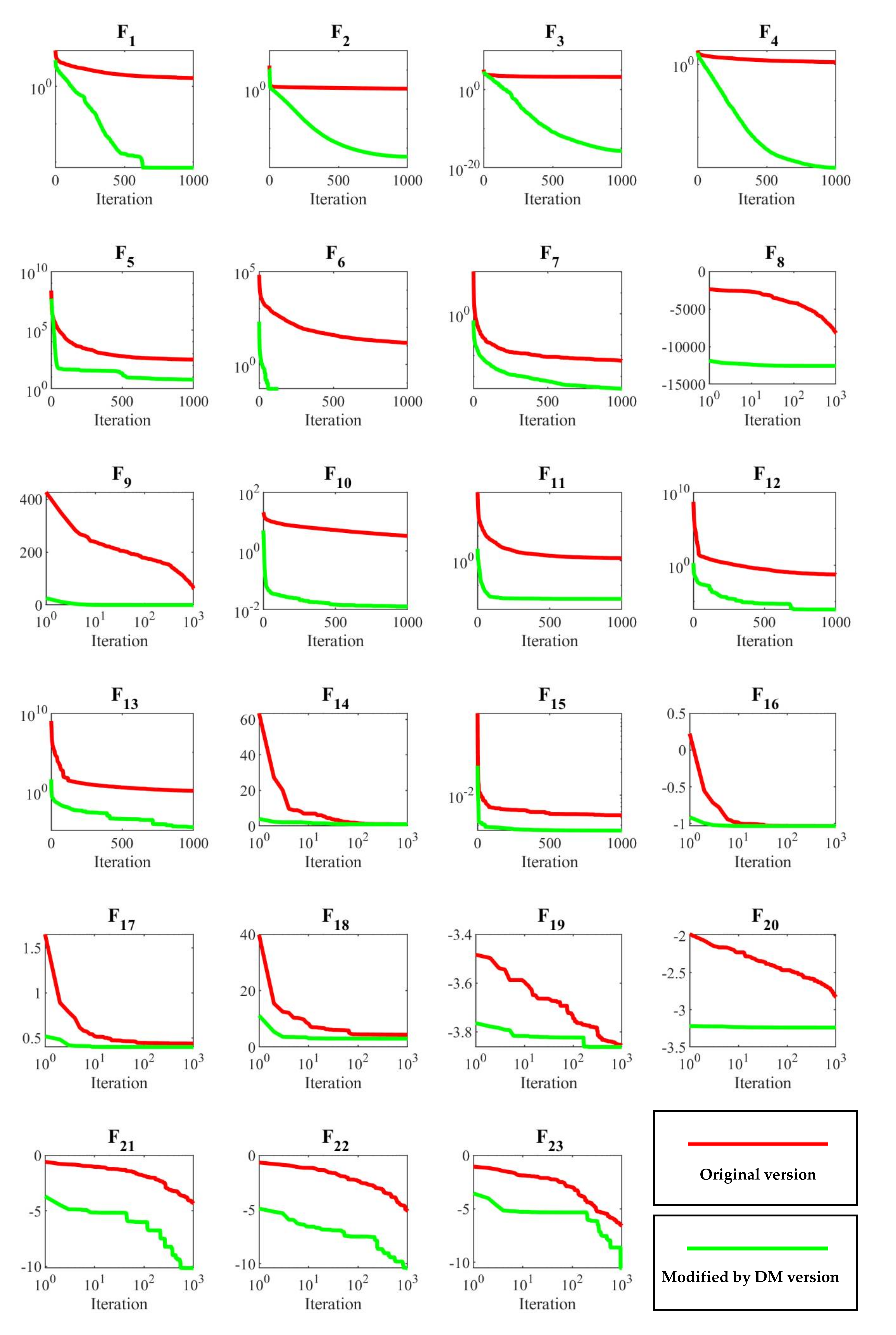
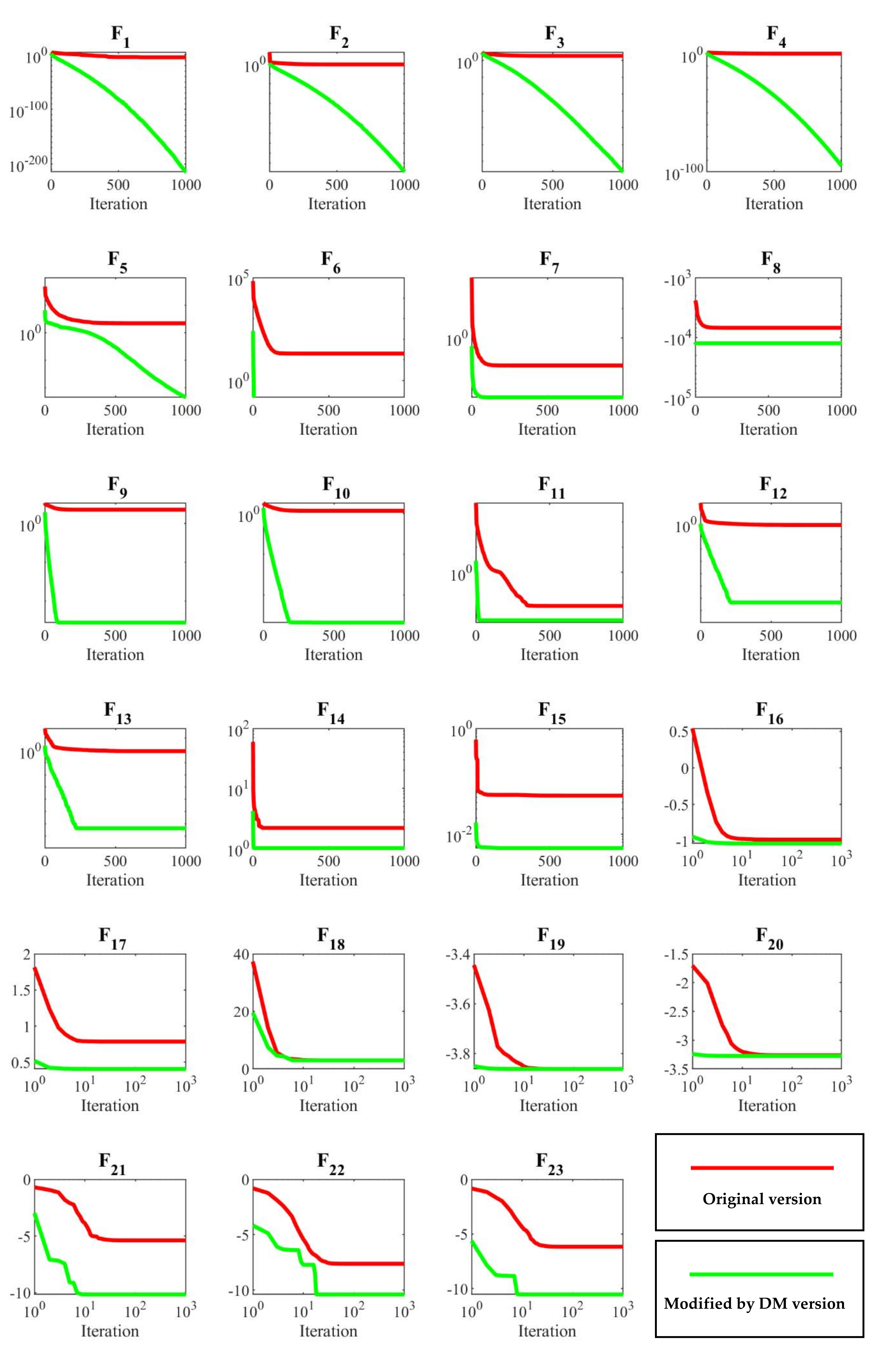
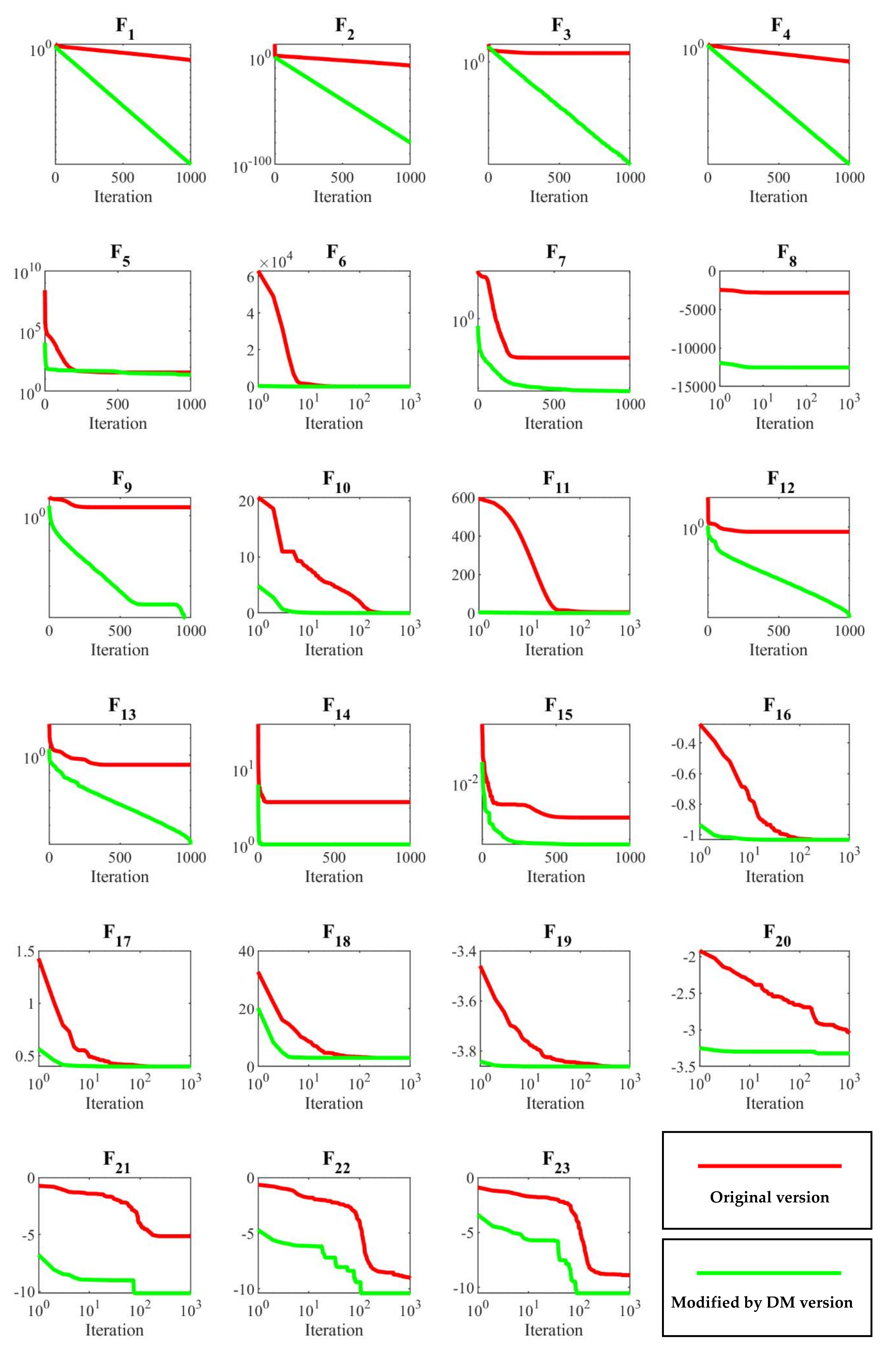
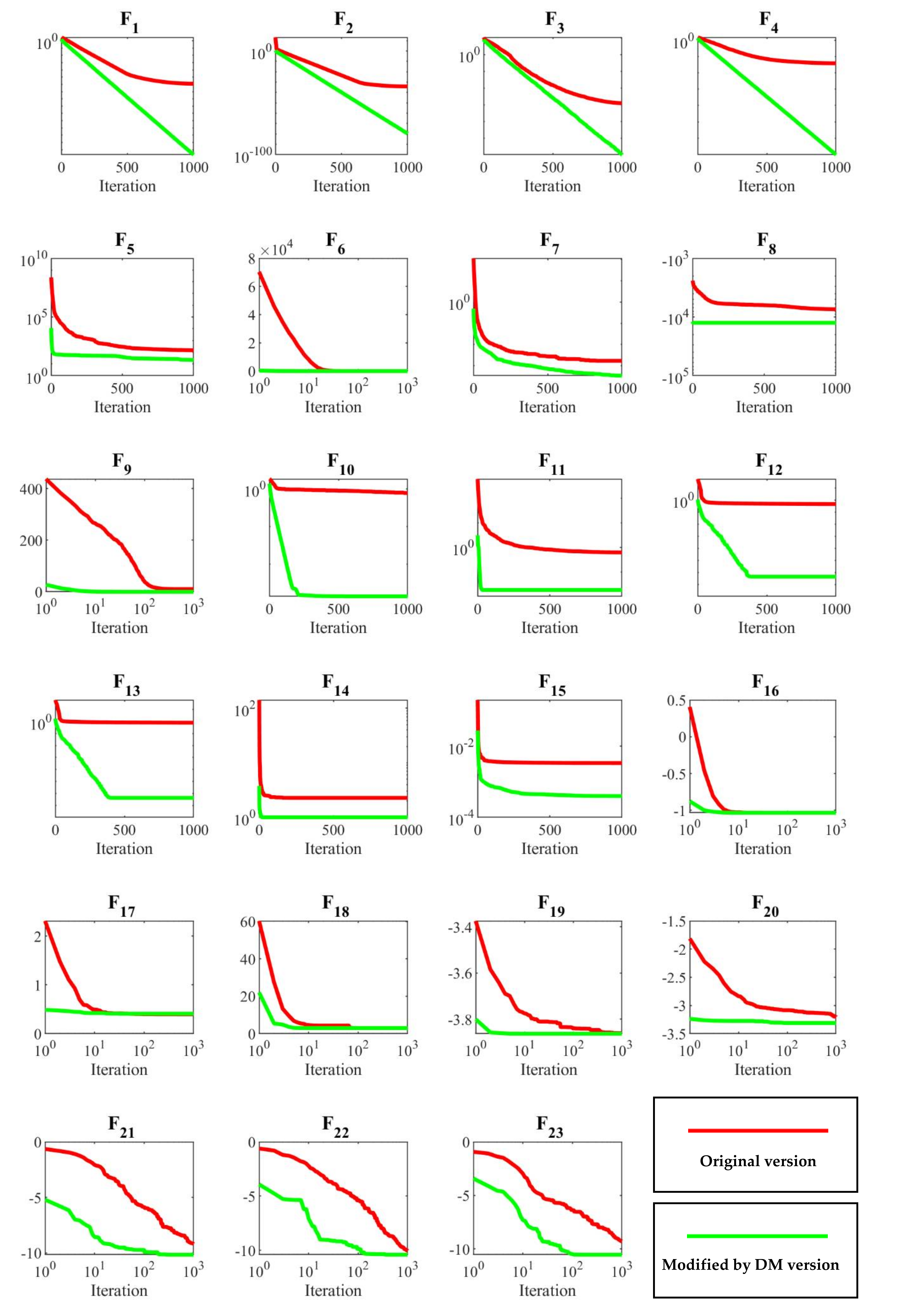
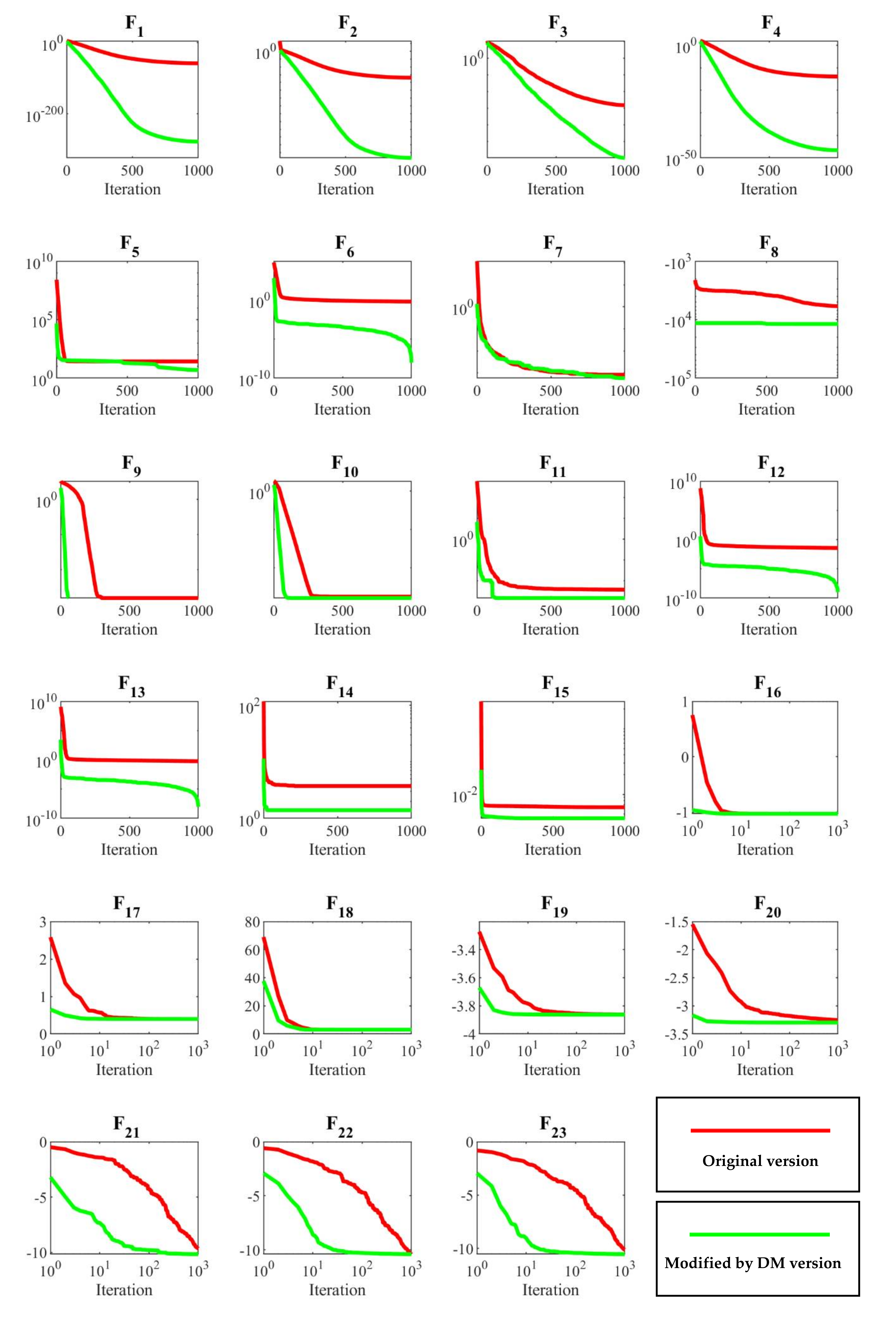
To further analyze the simulation results, the convergence curves of the optimization algorithms for the twenty-three objective functions are shown from
Figure 3,
Figure 4,
Figure 5,
Figure 6 and
Figure 7. In these figures, the convergence curves for the original and the modified versions are plotted simultaneously.
Computational time analysis in accessing the optimal solution is presented in
Table 7,
Table 8 and
Table 9. This analysis shows computational time for per iteration, per complete run, and the overall time required for the original and modified algorithm to achieve similar objective function value. In these tables, P.I. means per iteration, P.C. means per complete run, and the O.T.S. means overall time required for the original and modified algorithm to achieve similar objective function value.
4.3. Discussion
Exploitation and exploration abilities are two important indicators in evaluating optimization algorithms. The exploitation ability of an optimization algorithm means its power to provide a quasi-optimal solution. An algorithm that offers a better quasi-optimal solution than another algorithm has a higher exploitation ability. The unimodal objective functions F
1 to F
7, which have only one global optimal solution without local solutions, are applied to analyze the exploitation ability of optimization algorithms. The results presented in
Table 2,
Table 3,
Table 4,
Table 5 and
Table 6 show that the proposed DM by modifying the optimization algorithms is able to increase the exploitation ability of the optimization algorithms and as a result more suitable quasi-optimal solutions are provided by the modified version.
The exploration ability means the power of the optimization algorithm to scan the search space of an optimization problem. Given that the basis of optimization algorithms is random scanning of the search space, an algorithm that scans the search space more accurately is able move towards a quasi-optimal solution by escape from local optimal solutions. In the second and third category of objective functions F
8 to F
23, there are multiple local solutions besides the global optimum which are useful to analyze the local optima avoidance and an explorative ability of an algorithm.
Table 2,
Table 3,
Table 4,
Table 5 and
Table 6 show that the modified version with the DM of optimization algorithms has a higher exploration ability than the original version.
The convergence curves shown in
Figure 3,
Figure 4,
Figure 5,
Figure 6 and
Figure 7 visually show the effect of the proposed DM on the modifying the optimization algorithms. In these figures it is clear that the modified version moves with more convergence towards the quasi-optimal solution.
The simulation results of optimization algorithms to solve the optimization problems show that the modified version of the optimization algorithms with the DM are much more competitive than the its original version. Therefore, the proposed method has the ability to be implemented on a variety of optimization algorithms in order to solve various optimization problems.
The result of computational time analysis for both original and modified by DM versions is presented in
Table 7,
Table 8 and
Table 9. In these tables, three different time criteria are presented, which are the average time per iteration (P.I.), the average time per complete run (P.C.R.), and overall time required for the original and modified algorithm to achieve similar objective function value (O.T.S.). Due to the addition of a correction phase based on proposed DM, P.I. and P.C.R. have been increased compared to the original version.
Table 7 shows that except for four cases (TLBO: F
3, GWO: F
3, F
5, and F
7), in all unimodal objective functions, the modified version provides the final solution of the original version in less time.
Table 8 and
Table 9 show that the modified version of the studied algorithms for all F
8 to F
23 objective functions provides the final solution of the original version in less time.
5. Conclusions
There are various optimization problems in different sciences that should be optimized using the appropriate method. The optimization algorithm is one method to solve such problems, and it can provide a quasi-optimal solution by random scanning in the search space. Many optimization algorithms have been proposed by researchers which have been applied by scientists to solve optimization problems. The performance of optimization algorithms in achieving quasi-optimal solutions is improved by modifying optimization algorithms. In this paper, a new modification method has been presented for optimization algorithms called Dehghani method (DM). The main idea of the proposed DM is to improve and strengthen the best member of the population using the information of the population members. In DM, all members of a population, even the worst one, can contribute to the development of the population. The various stages of DM have been described and then has been modeled mathematically. The DM has been implemented on five different optimization algorithms including GA, PSO, GSA, TLBO, and GWO. The effect of the proposed method on modifying the performance of optimization algorithms in solving optimization problems has been evaluated on a set of twenty-three standard objective functions. In this evaluation, the results of optimizing the objective functions set has been presented for both the original and the modified by DM version of the optimization algorithms. The results of simulation and implementation of DM on the mentioned optimization algorithms with the aim of optimizing the optimization problems show that the proposed method improves the performance of the optimization algorithms. The optimization of different objective functions in the three groups unimodal, multimodal, and fixed-dimension multimodal functions indicates that the modified version with the proposed method is much more competitive than the original version. Moreover, the convergence curves visually show that the modified version moves with more convergence towards the quasi-optimal solution.
The authors suggest several ideas and proposals for future studies and perspectives of this study to researchers. The main potential for these ideas is to be found in modifying various optimization algorithms using DM. DM may also be used to overcome many objective real-life optimizations as well as multi-objective problems.
Author Contributions
Conceptualization, M.D., Z.M., A.D., H.S., O.P.M. and J.M.G.; methodology, M.D., Z.M. and A.D.; software, M.D., Z.M. and H.S.; validation, J.M.G., G.D., A.D., H.S., O.P.M., R.A.R.-M., C.S., D.S. and A.E.; formal analysis, A.D., A.E.; investigation, M.D. and Z.M.; resources, A.D., A.E. and J.M.G.; data curation, G.D.; writing—original draft preparation, M.D. and Z.M.; writing—review and editing, A.D., R.A.R.-M., D.S., C.S., A.E., O.P.M., G.D., and J.M.G.; visualization, M.D.; supervision, M.D., Z.M. and A.D.; project administration, A.D. and Z.M.; funding acquisition, C.S., D.S. and R.A.R.-M. All authors have read and agreed to the published version of the manuscript.
Funding
The current project was funded by Tecnológico de Monterrey and FEMSA Foundation (grant: CAMPUSCITY Project).
Conflicts of Interest
The authors declare no conflict of interest. The authors declare that they have no known competing financial interests or personal relationships that could have appeared to influence the work reported in this paper.
Abbreviations
| Acronym | Definition |
| ABC | Artificial Bee Colony |
| ACO | Ant Colony Optimization |
| ACROA | Artificial Chemical Reaction Optimization Algorithm |
| BA | Bat-inspired Algorithm |
| BBO | Biogeography-Based Optimizer |
| BH | Black Hole |
| BSS | Best-Suggested Solution |
| CS | Cuckoo Search |
| CSO | Curved Space Optimization |
| DM | Dehghani Method |
| DGO | Dice Game Optimizer |
| DGO | Darts Game Optimizer |
| DPO | Doctor and Patient Optimization |
| DE | Differential Evolution |
| DTO | Donkey Theorem Optimization |
| ES | Evolution Strategy |
| EPO | Emperor Penguin Optimizer |
| FOA | Following Optimization Algorithm |
| FGBO | Football Game Based Optimization |
| GA | Genetic Algorithm |
| GP | Genetic Programming |
| GO | Group Optimization |
| GOA | Grasshopper Optimization Algorithm |
| GSA | Gravitational Search Algorithm |
| GbSA | Galaxy-based Search Algorithm |
| GWO | Grey Wolf Optimizer |
| HOGO | Hide Objects Game Optimization |
| MLO | Multi Leader Optimizer |
| OSA | Orientation Search Algorithm |
| PSO | Particle Swarm Optimization |
| RSO | Rat Swarm Optimizer |
| RO | Ray Optimization |
| SHO | Spotted Hyena Optimizer |
| SGO | Shell Game Optimization |
| SWOA | Small World Optimization Algorithm |
| SS | Suggested Solution |
| TLBO | Teaching-Learning-Based Optimization |
| OF | Objective Function |
Appendix A
Table A1.
Unimodal objective functions.
Table A1.
Unimodal objective functions.
| |
| |
| |
| |
| |
| |
| |
Table A2.
Multimodal objective functions.
Table A2.
Multimodal objective functions.
| |
| |
| |
| |
| |
|
| |
Table A3.
Multimodal objective functions with fixed dimension.
Table A3.
Multimodal objective functions with fixed dimension.
| |
| |
| |
| |
| |
| |
| |
| |
| |
| |
References
- Dehghani, M.; Montazeri, Z.; Dehghani, A.; Ramirez-Mendoza, R.A.; Samet, H.; Guerrero, J.M.; Dhiman, G. MLO: Multi leader optimizer. Int. J. Intell. Eng. Syst. 2020, 13, 364–373. [Google Scholar]
- Dhiman, G.; Garg, M.; Nagar, A.; Kumar, V.; Dehghani, M. A novel algorithm for global optimization: Rat swarm optimizer. J. Ambient Intell. Humaniz. Comput. 2020. [Google Scholar] [CrossRef]
- Dehghani, M.; Mardaneh, M.; Guerrero, J.M.; Malik, O.P.; Kumar, V. Football game based optimization: An application to solve energy commitment problem. Int. J. Intell. Eng. Syst. 2020, 13, 514–523. [Google Scholar] [CrossRef]
- Dehghani, M.; Montazeri, Z.; Malik, O.P. Energy commitment: A planning of energy carrier based on energy consumption. Электрoтехника Электрoмеханика 2019, 4, 69–72. [Google Scholar] [CrossRef]
- Liu, J.; Dong, H.; Jin, T.; Liu, L.; Manouchehrinia, B.; Dong, Z. Optimization of hybrid energy storage systems for vehicles with dynamic on-off power loads using a nested formulation. Energies 2018, 11, 2699. [Google Scholar] [CrossRef]
- Carpinelli, G.; Mottola, F.; Proto, D.; Russo, A.; Varilone, P. A hybrid method for optimal siting and sizing of battery energy storage systems in unbalanced low voltage microgrids. Appl. Sci. 2018, 8, 455. [Google Scholar] [CrossRef]
- Ehsanifar, A.; Dehghani, M.; Allahbakhshi, M. Calculating the leakage inductance for transformer inter-turn fault detection using finite element method. In Proceedings of the 2017 Iranian Conference on Electrical Engineering (ICEE), Tehran, Iran, 2–4 May 2017; pp. 1372–1377. [Google Scholar]
- Dehghani, M.; Montazeri, Z.; Malik, O.P. Optimal sizing and placement of capacitor banks and distributed generation in distribution systems using spring search algorithm. Int. J. Emerg. Electr. Power Syst. 2020, 21, 20190217. [Google Scholar] [CrossRef]
- Dehghani, M.; Montazeri, Z.; Malik, O.P.; Al-Haddad, K.; Guerrero, J.M.; Dhiman, G. A new methodology called dice game optimizer for capacitor placement in distribution systems. Электрoтехника Электрoмеханика 2020. [Google Scholar] [CrossRef]
- Dehbozorgi, S.; Ehsanifar, A.; Montazeri, Z.; Dehghani, M.; Seifi, A. Line loss reduction and voltage profile improvement in radial distribution networks using battery energy storage system. In Proceedings of the IEEE 4th International Conference on Knowledge-Based Engineering and Innovation (KBEI), Tehran, Iran, 22 December 2017; pp. 215–219. [Google Scholar]
- Montazeri, Z.; Niknam, T. Optimal utilization of electrical energy from power plants based on final energy consumption using gravitational search algorithm. Электрoтехника Электрoмеханика, 2018, 4, 70–73. [Google Scholar] [CrossRef]
- Dehghani, M.; Mardaneh, M.; Montazeri, Z.; Ehsanifar, A.; Ebadi, M.; Grechko, O. Spring search algorithm for simultaneous placement of distributed generation and capacitors. Електрoтехніка Електрoмеханіка 2018, 6, 68–73. [Google Scholar] [CrossRef]
- Yu, J.; Kim, C.-H.; Wadood, A.; Khurshiad, T.; Rhee, S.-B. A novel multi-population based chaotic JAYA algorithm with application in solving economic load dispatch problems. Energies 2018, 11, 1946. [Google Scholar] [CrossRef]
- Sleesongsom, S.; Bureerat, S. Topology optimisation using MPBILs and multi-grid ground element. Appl. Sci. 2018, 8, 271. [Google Scholar] [CrossRef]
- Dehghani, M.; Montazeri, Z.; Ehsanifar, A.; Seifi, A.; Ebadi, M.; Grechko, O. Planning of energy carriers based on final energy consumption using dynamic programming and particle swarm optimization. Электрoтехника Электрoмеханика 2018, 5, 62–71. [Google Scholar] [CrossRef]
- Montazeri, Z.; Niknam, T. Energy carriers management based on energy consumption. In Proceedings of the IEEE 4th International Conference on Knowledge-Based Engineering and Innovation (KBEI), Tehran, Iran, 22 December 2017; pp. 539–543. [Google Scholar]
- Dehghani, M.; Mardaneh, M.; Malik, O.P.; Guerrero, J.M.; RMorales-Menendez, R.; Ramirez-Mendoza, A.; Matas, J.; Abusorrah, A. Energy commitment for a power system supplied by a multiple energy carriers system using following optimization algorithm. Appl. Sci. 2020, 10, 5862. [Google Scholar] [CrossRef]
- Kennedy, J.; Eberhart, R. Particle swarm optimization. In Proceeding of the IEEE International Conference on Neural Networks, Perth, WA, Australia; IEEE Service Center: Piscataway, NJ, USA, 1942; Volume 1948. [Google Scholar]
- Dorigo, M.; Stützle, T. Ant colony optimization: Overview and recent advances. In Handbook of Metaheuristics; Springer: Berlin/Heidelberg, Germany, 2019; pp. 311–351. [Google Scholar]
- Ning, J.; Zhang, C.; Sun, P.; Feng, Y. Comparative study of ant colony algorithms for multi-objective optimization. Information 2019, 10, 11. [Google Scholar] [CrossRef]
- Dhiman, G.; Kumar, V. Spotted hyena optimizer: A novel bio-inspired based metaheuristic technique for engineering applications. Adv. Eng. Softw. 2017, 114, 48–70. [Google Scholar] [CrossRef]
- Dehghani, M.; Montazeri, Z.; Dehghani, A.; Malik, O.P. GO: Group optimization. Gazi Univ. J. Sci. 2020, 33, 381–392. [Google Scholar] [CrossRef]
- Karaboga, D.; Basturk, B. Artificial bee colony (ABC) optimization algorithm for solving constrained optimization problems. In International Fuzzy Systems Association World Congress; Springer: Berlin/Heidelberg, Germany, 2007; pp. 789–798. [Google Scholar]
- Dehghani, M.; Mardaneh, M.; Malik, O. FOA: ‘Following’ optimization algorithm for solving power engineering optimization problems. J. Oper. Autom. Power Eng. 2020, 8, 57–64. [Google Scholar]
- Yang, X.-S. A new metaheuristic bat-inspired algorithm. In Nature Inspired Cooperative Strategies for Optimization (NICSO 2010); Springer: Berlin/Heidelberg, Germany, 2010; pp. 65–74. [Google Scholar]
- Dhiman, G.; Kumar, V. Emperor penguin optimizer: A bio-inspired algorithm for engineering problems. Knowl. Based Syst. 2018, 159, 20–50. [Google Scholar] [CrossRef]
- Gandomi, A.H.; Yang, X.-S.; Alavi, A.H. Cuckoo search algorithm: A metaheuristic approach to solve structural optimization problems. Eng. Comput. 2013, 29, 17–35. [Google Scholar] [CrossRef]
- Dehghani, M.; Mardaneh, M.; Malik, O.P.; NouraeiPour, S.M. DTO: Donkey Theorem Optimization. In Proceedings of the 27th Iranian Conference on Electrical Engineering (ICEE), Yazd, Iran, 30 April–2 May 2019; pp. 1855–1859. [Google Scholar]
- Sarzaeim, P.; Bozorg-Haddad, O.; Chu, X. Teaching-learning-based optimization (TLBO) algorithm. In Advanced Optimization by Nature-Inspired Algorithms; Springer: Berlin/Heidelberg, Germany, 2018; pp. 51–58. [Google Scholar]
- Saremi, S.; Mirjalili, S.; Lewis, A. Grasshopper optimisation algorithm: Theory and application. Adv. Eng. Softw. 2017, 105, 30–47. [Google Scholar] [CrossRef]
- Dehghani, M.; Mardaneh, M.; Guerrero, J.M.; Malik, O.P.; Ramirez-Mendoza, R.A.; Matas, J.; Vasquez, J.C.; Parra-Arroyo, L. A new “Doctor and Patient” optimization algorithm: An application to energy commitment problem. Appl. Sci. 2020, 10, 5791. [Google Scholar] [CrossRef]
- Mirjalili, S.; Mirjalili, S.M.; Lewis, A. Grey wolf optimizer. Adv. Eng. Softw. 2014, 69, 46–61. [Google Scholar] [CrossRef]
- Dehghani, M.; Montazeri, Z.; Saremi, S.; Dehghani, A.; Malik, O.P.; Al-Haddad, K.; Guerrero, J.M. HOGO: Hide objects game optimization. Int. J. Intell. Eng. Syst. 2020, 13, 216–225. [Google Scholar]
- Dehghani, M.; Montazeri, Z.; Malik, O.P.; Ehsanifar, A.; Dehghani, A. OSA: Orientation search algorithm. Int. J. Ind. Electr. Control Optim. 2019, 2, 99–112. [Google Scholar]
- Dehghani, M.; Montazeri, Z.; Malik, O.P.; Dhiman, G.; Kumar, V. BOSA: Binary orientation search algorithm. Int. J. Innov. Technol. Explor. Eng. 2019, 9, 5306–5310. [Google Scholar]
- Dehghani, M.; Montazeri, Z.; Malik, O.P. DGO: Dice game optimizer. Gazi Univ. J. Sci. 2019, 32, 871–882. [Google Scholar] [CrossRef]
- Dehghani, M.; Montazeri, Z.; Malik, O.P.; Givi, H.; Guerrero, J.M. Shell game optimization: A novel game-based algorithm. Int. J. Intell. Eng. Syst. 2020, 13, 246–255. [Google Scholar] [CrossRef]
- Dehghani, M.; Montazeri, Z.; Givi, H.; Guerrero, J.M.; Dhiman, G. Darts game optimizer: A new optimization technique based on darts game. Int. J. Intell. Eng. Syst. 2020, 13, 286–294. [Google Scholar] [CrossRef]
- Dehghani, M.; Montazeri, Z.; Dehghani, A.; Seifi, A. Spring search algorithm: A new meta-heuristic optimization algorithm inspired by Hooke’s law. In Proceedings of the 2017 IEEE 4th International Conference on Knowledge-Based Engineering and Innovation (KBEI), Tehran, Iran, 22 December 2017; pp. 210–214. [Google Scholar]
- Dehghani, M.; Montazeri, Z.; Dehghani, A.; Nouri, N.; Seifi, A. BSSA: Binary spring search algorithm. In Proceedings of the 2017 IEEE 4th International Conference on Knowledge-Based Engineering and Innovation (KBEI), Tehran, Iran, 22 December 2017; pp. 220–224. [Google Scholar]
- Moghaddam, F.F.; Moghaddam, R.F.; Cheriet, M. Curved space optimization: A random search based on general relativity theory. arXiv 2012, arXiv:1208.2214. [Google Scholar]
- Hatamlou, A. Black hole: A new heuristic optimization approach for data clustering. Inf. Sci. 2013, 222, 175–184. [Google Scholar] [CrossRef]
- Kaveh, A.; Khayatazad, M. A new meta-heuristic method: Ray optimization. Comput. Struct. 2012, 112, 283–294. [Google Scholar] [CrossRef]
- Alatas, B. ACROA: Artificial chemical reaction optimization algorithm for global optimization. Expert Syst. Appl. 2011, 38, 13170–13180. [Google Scholar] [CrossRef]
- Shah-Hosseini, H. Principal components analysis by the galaxy-based search algorithm: A novel metaheuristic for continuous optimization. Int. J. Comput. Sci. Eng. 2011, 6, 132–140. [Google Scholar]
- Du, H.; Wu, X.; Zhuang, J. Small-world optimization algorithm for function optimization. In International Conference on Natural Computation; Springer: Berlin/Heidelberg, Germany, 2006; pp. 264–273. [Google Scholar] [CrossRef]
- Karkalos, N.E.; Markopoulos, A.P.; Davim, J.P. Evolutionary-based methods. In Computational Methods for Application in Industry 4.0; Springer: Berlin/Heidelberg, Germany, 2019; pp. 11–31. [Google Scholar] [CrossRef]
- Mirjalili, S. Biogeography-based optimisation. In Evolutionary Algorithms and Neural Networks; Springer: Berlin/Heidelberg, Germany, 2019; pp. 57–72. [Google Scholar] [CrossRef]
- Storn, R.; Price, K. Differential evolution-A simple and efficient adaptive scheme for global optimization over continuous spaces. Berkeley ICSI 1995, 11, 341–359. [Google Scholar] [CrossRef]
- Tang, K.-S.; Man, K.-F.; Kwong, S.; He, Q. Genetic algorithms and their applications. IEEE Signal Process. Mag. 1996, 13, 22–37. [Google Scholar] [CrossRef]
- Beyer, H.-G.; Schwefel, H.-P. Evolution strategies—A comprehensive introduction. Nat. Comput. 2002, 1, 3–52. [Google Scholar] [CrossRef]
- Koza, J.R. Genetic Programming: A Paradigm for Genetically Breeding Populations of Computer Programs to Solve Problems. PhD Thesis, Stanford University, Stanford, CA, USA, 1990. [Google Scholar]
- Rashedi, E.; Nezamabadi-Pour, H.; Saryazdi, S. GSA: A gravitational search algorithm. Inf. Sci. 2009, 179, 2232–2248. [Google Scholar] [CrossRef]
- Dhghani, M.; Montazeri, Z.; Dhiman, G.; Malik, O.P.; Morales-Menendez, R.; Ramirez-Mendoza, R.A.; Dehghani, A.; Guerrero, J.M.; Parra-Arroyo, L. A spring search algorithm applied to engineering optimization problems. Appl. Sci. 2020, 10, 6173. [Google Scholar] [CrossRef]
| Publisher’s Note: MDPI stays neutral with regard to jurisdictional claims in published maps and institutional affiliations. |
© 2020 by the authors. Licensee MDPI, Basel, Switzerland. This article is an open access article distributed under the terms and conditions of the Creative Commons Attribution (CC BY) license (http://creativecommons.org/licenses/by/4.0/).


 ,
, 


